Comparison of Single-Trait and Multi-Trait GBLUP Models for Genomic Prediction in Red Clover

Abstract

Red clover (Trifolium pratense) is a perennial forage legume wildly used in temperate regions, including northern Europe. Its breeders are under increasing pressure to obtain rapid genetic gains to meet the high demand for improved forage yield and quality. One solution to increase genetic gain by reducing time and increasing accuracy is genomic selection. Thus, efficient genomic prediction (GP) models need to be developed, which are unbiased to traits and harvest time points. This study aimed to develop and evaluate single-trait (ST) and multi-trait (MT) models that simultaneously target more than one trait or cut. The target traits were dry matter yield, crude protein content, net energy for lactation, and neutral detergent fiber. The MT models either combined dry matter yield with one forage quality trait, all traits at one cut, or one trait across all cuts. The results show an increase with MT models where the traits had a genetic correlation of 0.5 or above. This study indicates that non-additive genetic effects have significant but varying effects on the predictive ability and reliability of the models. The key conclusion of this study was that these non-additive genetic effects could be better described by incorporating genetically correlated traits or cuts.

1. Introduction

Forages are among the main crops grown in the Nordic Region of Europe and are commonly grown as a mixture of grasses and legumes. One of the major forage legumes is red clover (Trifolium pratense), which is highly valued because of its high protein content and multiple ecological services [1,2]. (Red clover is a diploid species (2n = 14 chromosomes) with a genome size of 420 Mbp [3]. However, tetraploid genotypes have been developed via chemical treatment, which later were developed into tetraploid cultivars through further breeding [4]. Crossing between diploids and tetraploids is possible but with a low success rate [5]. Tetraploids have a higher biomass yield and higher persistence and resilience than diploids, but their seed yield is lower [6,7]. Because of differences in genetics and target traits for breeding, tetraploids and diploids are bred under different breeding programs. Additionally, red clover populations that significantly differ in their rate of maturity are usually bred under different breeding programs, as red clover is highly affected by growing conditions such as temperature variations across and between seasons [8]. However, population genetics research shows that there was a lack of population structure within the separate breeding programs [9,10].

Despite the crop’s significance, new red clover cultivars with improved forage yield and nutritional quality have not been adequately developed to meet increasing demands. Current breeding programs largely rely on solely phenotypic data to select desirable parents for breeding. This approach is time-consuming, as red clover is a perennial crop and complete phenotypic evaluation takes several years. Hence, the process of developing a new cultivar from the first crossing to market introduction can take over 20 years [11]. By introducing genomic selection, generation time can be reduced significantly compared with the progeny testing-based method. This increases genetic gain per given time [12].

Implementing genomic selection in forage crops is not without challenges [13]. One major hurdle in red clover is its outcrossing nature. Hence, developing inbred lines is impossible because of strong self-incompatibility [14]. Thus, the genetic makeup of populations is of higher interest than that of individuals.

Futschik and Schlötterer [15] showed that sampling a number of individuals from a population and sequencing them as one sample, a method referred to as “pool-seq”, gave a better estimate of population-wide allele frequency than individual sequencing carried out at the same price point. Each pool consists of an equal amount of leaf tissue that is treated as one sample through DNA extraction, sequencing, and variant calling. The ration between reads is proportional to the allele frequency in the pooled individuals and is used as an estimate of population-wide allele frequencies.

Generating genomic data can therefore be performed at the population level, and the allele frequency can be used to model additive genetic variance. Genomic predictions on single traits have been successfully performed using additive models with allele frequencies as genetic input data for both red clover [16,17] and ryegrass [18].

To the best of our knowledge, genomic prediction (GP) models in red clover have only been used to predict traits independently or as a summary across one or multiple years [17,19] (Nay et al., 2023, Skøt et al., 2024). Though total forage yield is the overall goal, the difference in forage yield between cuts is important as red clover is grown together with other crops and there is an interest in having equal ratios of crops within the forage silage. The difference in cuts across seasons is a measurement of persistence, a key trait for northern cultivars. Additionally, developing red clover cultivars with high forage quality traits is critical because forage quality has significant impacts on livestock health and performance. However, forage quality traits are often negatively correlated with biomass yield [20]. Hence, a better understanding of the correlation between desirable traits is crucial in forage improvement programs. However, studies of this nature are often deprioritized because of high analysis costs, lack of agreement on more significant attributes, and multiple competing goals. In this study, forage yield was measured as dry matter yield per plot, which is the main target trait in red clover breeding.

The forage quality traits targeted in this study were crude protein content, net energy for lactation (NEL), and neutral detergent fiber (NDF). NEL is an estimation of how much of the absorbed energy from the feed goes to lactation. NDF is an estimate of the fiber content of the feed, primarily cellulose, hemicellulose, and lignin, compounds that are only partially digested. Hence, a higher level of NDF lowers the level of available calories, NEL, in the feed. High NDF may suggest more stems than leaves [21]. This is because leaves usually contain higher protein concentrations. Agriculturally beneficial traits, such as yield and quality, are often multi-genic traits. They are controlled by many genes and DNA motifs located at various independent loci throughout the genome. These are called quantitative trait loci (QTL). Quantitative genetics aims to map and describe the effects of QTL within and between populations. This is accomplished by describing the observed variance in the phenotype as a sum of the genetic variance, the environmental variance, and the variance due to genotype-by-environment interactions at a trial site or in the native environment.

$$P=G+E+G\times E$$

This simple formula by Falconer and Mackay [22] lays the ground for breeding. The goal here is to estimate the genotype parameter (G) using phenotype data (P), an environmental effect (E), and any interactions between the genotype and environment (G × E) so that new phenotypes can be estimated using only G and E information. In genomic selection (GS), kinship information, which is often based on marker information, is used to estimate G. Thus, fewer experiments, such as replicated field trials, are needed to estimate the relationship between G and E. Furthermore, the introduction of GS can significantly reduce the time needed to develop a cultivar by substituting decisions based on phenotypic information with decisions based on genomic information. This significantly shortens evaluation times. GS can be performed using either a few markers associated with a specific trait (marker-assisted selection, MAS) or many markers across the genome to predict genetic breeding values (genomic prediction, GP). GP is built on models that utilize DNA marker information to predict genotypic values via best linear unbiased prediction models (BLUP). Mixed linear models can account for both fixed and random effects. Hence, it corrects for variation across trials and variation in residuals for within-trial spatial effects in addition to estimating genotypic effects.

Prediction models that add genetic marker data in the form of a kinship or genetic relationship matrix (GRM) are referred to as GBLUP. These models can be univariate (one response) or multivariate (two or more responses). Multivariate models, also called multi-trait models (MT), have the advantage of enhancing prediction accuracy as they “borrow” information on genetic relationships between individuals using genetic correlations between traits. Nonetheless, this depends on estimates of the genetic correlation between the traits. MT models have been successfully implemented in a variety of crops, such as wheat and potato [23,24], in which the increase in accuracy was attributed to the correlation between traits. Models based on the measurement of a single trait across different time points are referred to as longitudinal models. As with MT models, the correlation between time points is utilized for increased predictive ability in longitudinal models.

This study aimed to compare ST and MT models to examine the potential of MT models for increasing the prediction accuracy of key traits in red clover breeding.

2. Materials and Methods

2.1. Plant Material

This study used 488 red clover breeding accessions from the Swedish agricultural company Lantmännen (Sweden) and 44 accessions from NordGen (Nordic Genetic Resources Center, Alnarp, Sweden). Lantmännen accessions consisted of cultivars, and full or half-sib F2 families as well as synthetic populations. NordGen accessions were composed of wild populations, landraces, and cultivars. In total, 532 accessions were used for genotyping and field trial-based phenotyping.

2.2. Planting, Sampling, and DNA Extraction

Seeds of each accession were planted in a greenhouse at the Swedish University of Agricultural Sciences (SLU), Department of Plant Breeding, Alnarp, for DNA extraction. For planting, 50-cell (5 × 10) plastic seedling trays filled with soil were used. Leaf tissue was sampled from the first true leaf of a two-week-old seedling. The leaf tissue samples were collected using a BioArk leaf collection kit from LGC Biosearch Technologies. Two leaf discs were sampled with a 2 mm punch from 200 individuals per accession and pooled into a well in a 96-well sampling plate. Hence, each accession was represented by a single pool of 400 leaf discs from 200 seedlings. Following leaf collection, DNA was extracted from each pool and genotyped at LGC Biosearch Technologies (Berlin, Germany). A Sbeadex plant kit was used to extract high-quality genomic DNA for genotyping.

2.3. Genotyping-by-Sequencing (GBS) and Read Pre-Processing

A GBS library was constructed using PstI (5′-CTGCA/G-3′, a six-base cutter) and MseI (5′-T/TAA-3′, a four-base cutter) restriction enzymes as recommended by LGC Biosearch Technologies. By combining PstI-MseI, it was possible to obtain a fragment size distribution suitable for sequencing on Illumina platforms with a mean insert size of about 180 bp. A 150 bp paired-end GBS was performed on Illumina NextSeq 500/550 v2 and NovaSeq 6000 NGS platforms to generate the reads. After sequencing, multi-step read pre-processing was performed. The base calls were demultiplexed into FASTQ files according to their barcodes using Illumina’s bcl2fastq 2.17.1.14 software, and their enzyme restriction sites were verified. A subsequent step involved clipping sequencing adapter remnants from all reads and discarding reads with a final length below 20 bases and those that contained mismatching restriction enzyme sites. Then, reads were trimmed to achieve a minimum Phred quality score of 20 for a window of ten bases. Following this, FastQC reports of all FASTQ files were developed and read counts of all samples were generated.

2.4. Read Alignment and SNP Discovery

A combined alignment of high-quality reads of all samples against the red clover reference genome [25] in coordinate-sorted BAM format was performed with BWA-MEM version 0.7.12 [26]. Following this, variant discovery and genotyping of samples was performed with Freebayes v1.0.2-16 [27]. The specific parameters for variant discovery and genotyping included a base quality of at least 10, a read mismatch limit of 3, coverage of at least 5, an allele count of at least 4, and a ploidy of 2 or 4. The variants, SNPs, were then filtered for a read count of at least 50, a minimum allele frequency of 5%, and observations in at least 50% of the accessions.

2.5. Field Trials and Phenotyping

The 532 accessions were established in an augmented design-based field trial across three locations in Sweden, of which 528 accessions (352 diploids and 176 tetraploids) were non-replicated and 4 were used as checks. The checks included two diploid cultivars (SW Ares and SW Yngve) and two tetraploid cultivars (Vicky and Peggy). The 528 accessions were split into three subsets based on their ploidy level and maturity time. Diploid accessions were grouped into late-maturing type and middle-late-maturing type depending on their flowering time points. Because of differences in growing conditions, such as differences in temperature and daylength within and across seasons, late-maturing and middle-late-maturing diploids needed to be separated into two data sets. The late-maturing diploids (176 accessions) were sown at two locations in northern Sweden: Ås (63°14′51.7″ N 14°33′45.9″ E) and Lännäs (63°09′46.3″ N 17°39′31.0″ E). The middle-late-maturing diploids (176 accessions) were sown at the following locations in southern Sweden: Rådde (57°36′20.628″ N, 13°15′8.532″ E) and Svalöv (55°55′20.2″ N 13°07′16.4″ E). The tetraploids (176 accessions) were sown at three locations covering northern and southern Sweden (Lännäs, Rådde, and Svalöv). For simplicity, the three subsets are hereafter called late diploids, middle-late diploids, and tetraploids.

The augmented design-based trial for each subset at each location was composed of four blocks of 52 plots each. In each block, 44 accessions (non-replicated) and two of the four checks (according to their ploidy level), each replicated four times (44 + (2 × 4) = 52), were sown. Sowing was performed at a seeding rate of 800 seeds/m² for diploids and 740 seeds/m² for tetraploids, which is a standard rate for red clover in this area. The trials were established in the spring of 2020 at all locations. The field trials were managed with standard methods for sowing, harvesting, fertilizing, and pest management according to the protocols of the trial sites. The trial was fertilized in spring after each harvest. The fertilizer applied contained phosphorus and potassium but not nitrogen. Weed management was performed as standard with spray application using the appropriate active substance and timing for the specific weed, which was specific to each trial site. The first biomass harvests were conducted in mid-June in Svalöv, mid-to-late June in Rådde and Lännäs, and late June in Ås in 2021. These were according to the regular forage harvesting time and weather conditions for that year at each location determined by growth rate and weather conditions (Figure 1). The second biomass harvests were conducted in early August in Svalöv and Ås and in late July in Rådde and Lännäs in 2021. The third harvests were conducted in late September to early October in Svalöv, in early September in Rådde, and in late August in Lännäs in 2021. The fourth, fifth, and sixth harvests were performed in 2022 during the same period as the first, second, and third harvests, respectively. Harvests at Ås were only conducted twice per season because of the short growing season. The dry matter (DM) yield of each plot was estimated by collecting freshly cut samples, weighing them, drying them, and weighing them again. The first three harvests from all sites were analyzed for forage quality. Crude protein (CP) and NDF were analyzed using the NIR System 6500 (Foss, Hillerod, Denmark) with fg2019.eqa calibrations [28] (Association of German Agricultural Analytic and Research Institutes, VDLUFA, Germany). The reference method for NDF was according to Van Soest, Robertson, and Lewis [29] omitting amylase and sodium sulfite.

Net energy for lactation (NEL, MJ) was calculated as follows, according to GFE (2001):

$$NEL\left({\displaystyle \frac{MJ}{kg}}\right)=0.6\left[1+0.004\left(q-57\right)\right]\times ME$$

where

$$q={\displaystyle \frac{ME}{GE}}\times 100$$

where

$$\begin{gathered} ME\left({\displaystyle \frac{MJ}{kg}}\right)=0.021503\times CP+0.032497\times EE-0.021071\times CF \\ +0.016309\times starch+0.014701\times organic residue \end{gathered}$$

and

$$G\left({\displaystyle \frac{MK}{kg}}\right)\times 0.0239\times CP+0.0398\times EE+0.0201\times CF+0.0175\times NFE.$$

The units for CP, ether extract (EE), crude fiber (CF), nitrogen free extract (NFE), starch, and organic residue are g/kg. An organic residue is dry matter that does not include crude ash, crude protein, crude fiber, or crude starch. It consists primarily of non-starch carbohydrates.

2.6. Population Structure and Phenotypic Data Evaluation

Allelic frequency data were used to calculate Nei’s standard genetic distance between the accessions as in Osterman et al. [10] but separately for diploids and tetraploids using R software v. 4.3.1 [30]. The genetic distance data were then used to construct neighbor-joining (NJ) trees to assess the population structure in the data using the nj() function in the R package adegenet [31], which was visualized using ggtree [32].

The phenotypic data were first corrected for environmental effects using a linear mixed model (more details in the next section) and then evaluated for each trait at each cut using principal component analysis (PCA). Any correlations between traits were illustrated using Pearson correlations on a heatmap with the Complex Heatmap package [33].

2.7. The Different Models

All models were based on the additive linear mixed model

$$\mathit{y}=\mathit{X}\mathit{\beta }+\mathit{Z}\mathit{u}+\epsilon$$

where y is a n × 1 vector of responses, where n is the number of observations in the model. For the single-trait model, n corresponds to the number of accessions, while for the multi-trait and longitudinal models, n is the number of accessions times the number of traits/cuts tested. On the right-hand side are the fixed effects β and random effects u as well as a residual Ɛ, for which

$$\left[\begin{array}{c}u\\ \epsilon \end{array}\right]~N\left(\left[\begin{array}{c}0\\ 0\end{array}\right],\left[\begin{array}{cc}\mathit{G}\left({{\mathit{\sigma }}_g}^2\right)& 0\\ 0& {\mathit{R}}_v\left({{\mathit{\sigma }}_r}^2\right)\end{array}\right]\right)$$

Hence, u and Ɛ are normally distributed with a mean of 0 and a variance of G, as a function of genetic variance (${{\mathit{\sigma }}_g}^2$) and R as a function of residual variance (${\mathit{\sigma }}_r$). X and Z are index matrices connecting fixed and random effects to each observation. They contain the same number of rows as there are records and the same number of columns as there are effects minus one (since the first effect is treated as the intercept). The LMM’s system of equations is then solved using Henderson’s MME as

$$\left|\begin{array}{cc}\mathit{X}\prime \mathit{X}& \mathit{X}\prime \mathit{Z}\\ \mathit{Z}\prime \mathit{X}& {\mathit{Z}}^{\prime }\mathit{Z}+{\mathit{G}}^{-1}g\end{array}\right|\left|\begin{array}{c}\mathit{\beta }\\ \mathit{u}\end{array}\right|=\left|\begin{array}{c}\mathit{X}\prime \mathit{y}\\ \mathit{Z}\prime \mathit{y}\end{array}\right|$$

where X and Z are the index matrices above, G is the genetic relationship matrix as the realized additive genetic relationship matrix, and $g={\displaystyle \frac{{\sigma }_e^2}{{\sigma }_g^2}}$ is estimated from REML when fitting the LMM. The system of equations can be solved for Best Unbiased Linear Estimate (BLUE) for the fixed effects or Best Linear Unbiased Predictor (BLUP) for the random effects as

$$\mathit{\beta }=\left({\mathit{X}}^{\prime }{\mathit{V}}^{-1}\mathit{X}\right)-\mathit{X}\prime {\mathit{V}}^{-1}\mathit{y}$$

and

$$\mathit{u}={\sigma }_g^2\mathit{G}\mathit{Z}\prime {\mathit{V}}^{-1}\left(\mathit{y}-\mathit{X}\mathit{\beta }\right)$$

where

$$\mathit{V}={\sigma }_g^2\mathit{Z}\mathit{G}{\mathit{Z}}^{\prime }+{\sigma }_e^2\mathit{I}$$

This study used five different models, one to correct the phenotypic values based on environments and local spatial effects and one to determine Genomic Estimated Breeding Values (GEBVs). Step 1 adjusted the phenotypic values for any environmental variance and G × E variance to obtain the genotypic values. This was performed by setting the genotypes as fixed effects and the random effects as

$${\mathsf{\Sigma }}_u={\mathsf{\Sigma }}_{location}+{\mathsf{\Sigma }}_{location}⨂{\mathsf{\Sigma }}_{block}+{\mathsf{\Sigma }}_{location}⨂{\mathsf{\Sigma }}_{row}+{\mathsf{\Sigma }}_{location}⨂{\mathsf{\Sigma }}_{column}+{\mathsf{\Sigma }}_{location}⨂{\mathsf{\Sigma }}_{genotype}$$

with each term having a homogenous variance as

$$\mathsf{\Sigma }=\left[{\sigma }_{ij}^2\right] : \left\{\begin{array}{cc}{\sigma }_{ii}& \forall i\\ {\sigma }_{ij}={\sigma }_{ji}& i\ne j\end{array}\right\}$$

From the model, the best linear unbiased estimators (BLUEs), one for each accession, were calculated and used as responses in the following models. The other four models were single-trait (ST), single-trait-longitudinal (ST_L), multi-trait with two traits considered simultaneously (MT₁), and multi-trait with four traits considered simultaneously (MT₂).

Step 2 depended on the model structure, where the ST had a random variance of ${\mathsf{\Sigma }}_{genotype}$ with a given variance structure as a Gaussian kernel, which was defined as the covariance between two subjects $S_i$ and $S_j$ as

$$k\left(S_i, S_j\right)=\exp \left(-{\displaystyle \frac{{\Vert S_i-S_j\Vert }^2}{\rho }}\right); \rho >0$$

ρ was estimated by visual optimization so that the matrix values spanned 0 to 1 and a heatmap showed some clustering patterns. The resulting covariance matrix was used as the GRM.

The ST_L model had a fixed effect partitioned for the different cuts, i.e., time points as $\beta =\left[{\beta }_1,{\beta }_{2,}\dots ,{\beta }_c\right]$ with c equaling 4 (2 cuts per year) for the late diploids and 6 (3 cuts per year) for the middle-late diploids and the tetraploids when yield was the response. For a forage quality trait, c was halved since those data were only measured during the first year. The random effects were

$${\mathsf{\Sigma }}_u={\mathsf{\Sigma }}_{genotype}+{\mathsf{\Sigma }}_{geotype}⨂{\mathsf{\Sigma }}_{cut}$$

where ${\mathsf{\Sigma }}_{genotype}$ is the GRM variance structure and ${\mathsf{\Sigma }}_{cut}$ has a factor analytical model

$${\mathsf{\Sigma }}_{cut}=\mathsf{\Gamma }\mathsf{\Gamma }\prime$$

in which ${\mathsf{\Gamma }}_{\left(\omega \times k\right)}$ is a matrix of loadings, ω is the number of cuts, and k is the factor rank, where k = 2. The residuals were partitioned over each cut and modeled as

$${\mathsf{\Sigma }}_{\epsilon }={\mathsf{\Sigma }}_{units}⨂{\mathsf{\Sigma }}_{cut}$$

The MT₁ model was modeled between the yield and one forage quality trait at a single time point. The fixed effect was partitioned into two, one for each trait. The variance model was

$${\mathsf{\Sigma }}_u={\mathsf{\Sigma }}_{genotype}+{\mathsf{\Sigma }}_{geotype}⨂{\mathsf{\Sigma }}_{trait}$$

where ${\mathsf{\Sigma }}_{genotype}$ is the GRM variance structure and ${\mathsf{\Sigma }}_{trait}$ has a heterogeneous covariance structure as

$${\mathsf{\Sigma }}_{trait}=\left[{\sigma }_{ij}\right] : \left\{\begin{array}{cc}{\sigma }_{ii}={\sigma }_i^2& i=1, \dots \omega \\ {\sigma }_{ji}={\sigma }_{ij}& i\ne j\end{array}\right\}$$

in which ω = 2 and i = 2. The residuals were considered independent. However, for the MT₂ model, the increase in the number of traits made it possible to model residuals per trait as

$${\mathsf{\Sigma }}_{\epsilon }={\mathsf{\Sigma }}_{units}⨂{\mathsf{\Sigma }}_{trait}$$

The MT₂ model was formulated as MT₁ except ω = 4 and i = 4. The development and final selection of all the above models were based on Akaike information criterion (AIC) and Bayesian information criterion (BIC) as well as having residuals that fulfilled the criteria of $\epsilon ~N\left(0, {\sigma }_r^2\right)$.

2.8. Predictive Ability and Reliability

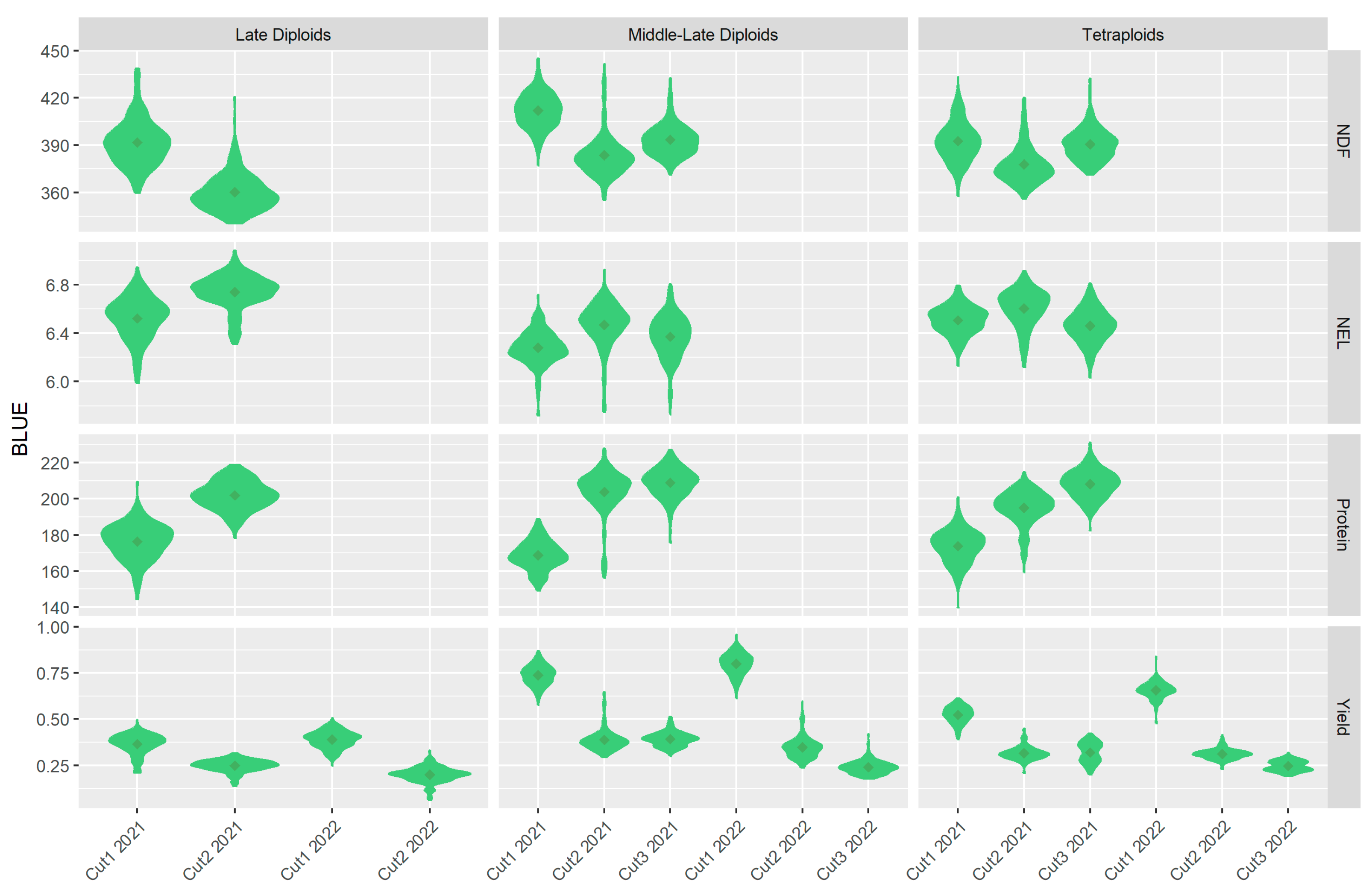
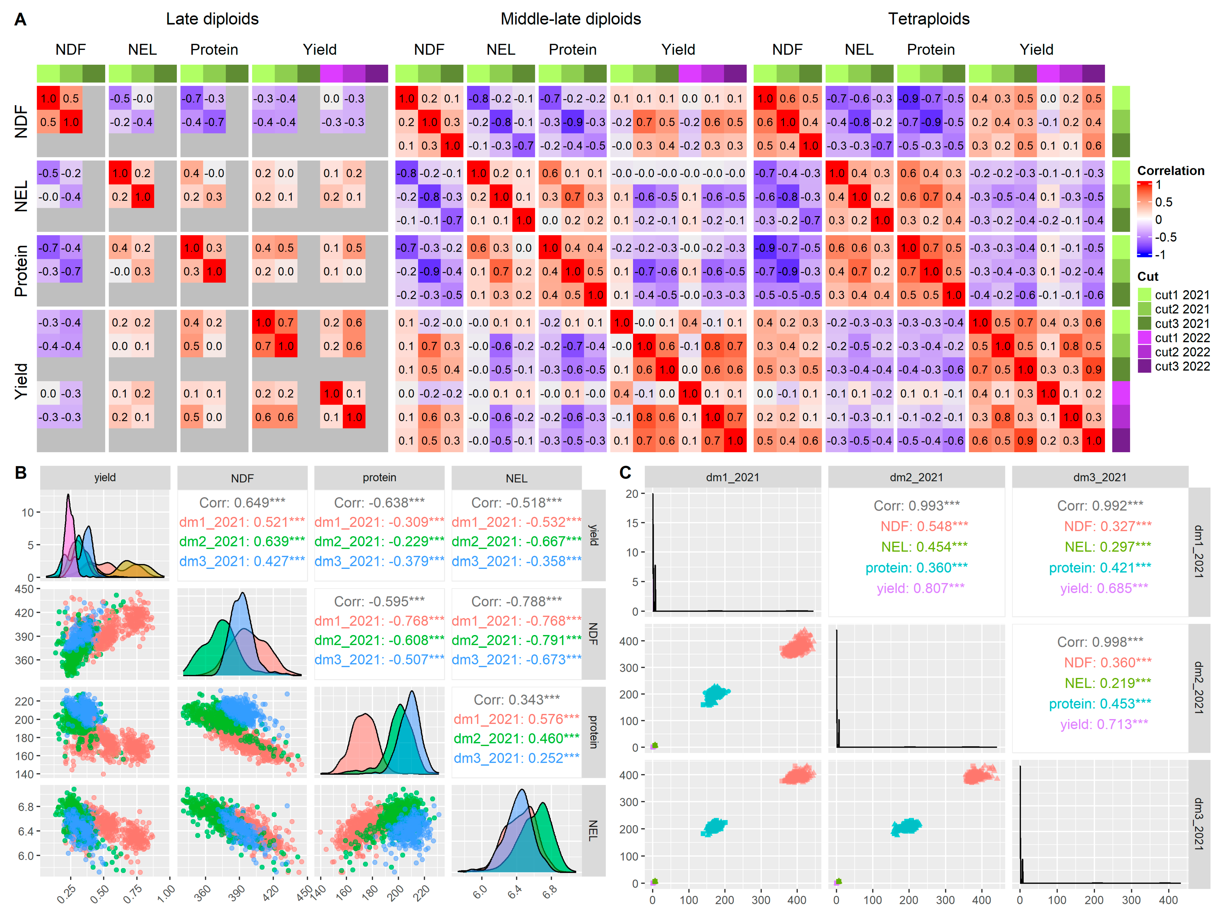
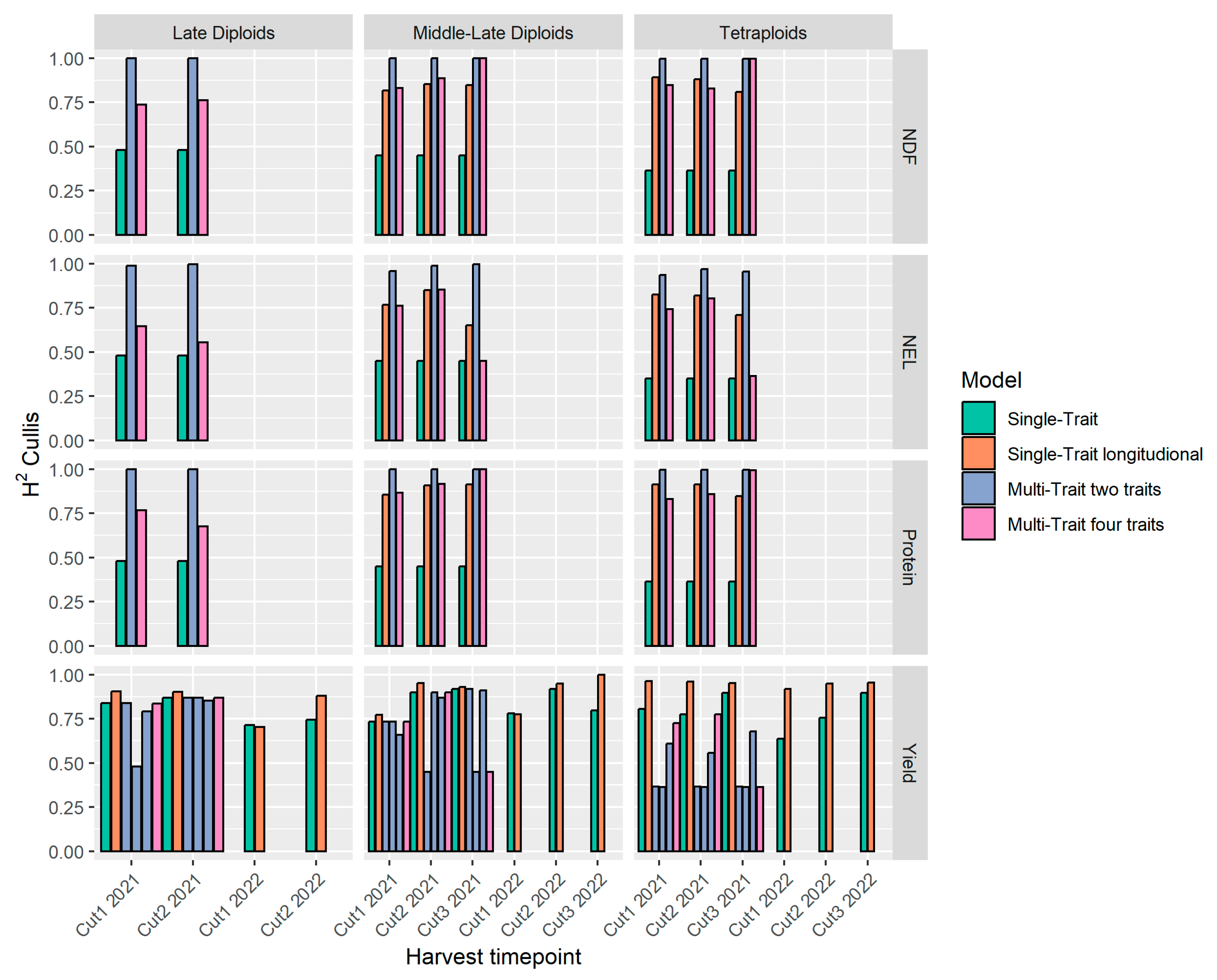
The genetic variation was estimated as

$${{\sigma }_g}^2={{\sigma }_{genetic}}^2+{{\sigma }_{genetic:trait}}^2$$

where ${{\sigma }_{genetic:trait}}^2$ was specific for each trait.

Since the factor analytical model in S_TL is a correlation model, the correlation between cuts was recalculated to variance by multiplying the estimated correlation matrix of the cuts with its transpose and taking the diagonal. For MT₁ and MT₂, the variance was calculated from the given variance components.

The predictions for validation and estimation of predictive ability were performed using 10-fold cross-validation, replicated 100 times. The predictive ability was measured as the Pearson’s correlation between the mean of the predicted BLUPs across all 100 iterations and the corrected phenotype.

$$r{\left(g_i, {\widehat{g}}_i\right)}^2=1-{\displaystyle \frac{PEV\left({\widehat{a}}_i\right)}{{\widehat{\sigma }}_g^2}}$$

The broad-sense heritability (H²) was calculated according to Cullis et al. [34] and used as reliability, following the equation

$$H_{Cullis}^2=1-{\displaystyle \frac{{\overline{V}}_{\mathsf{\Delta }}^{BLUP}}{2\ast {\sigma }_g^2}}$$

3. Results

3.1. Genotyping

The GBS resulted in a total of 3.9 billion read pairs, with an average of 7.3 million reads per sample. The average mapping rate of reads to the reference genome was 62%. All four checks and 176 tetraploids were successfully sequenced. Among the diploids, 171 and 165 middle-late and late diploid accessions were successfully sequenced. Five middle-late diploid and 11 late diploid accessions failed. Following all quality control and filtering steps, 8107 and 13,544 high-quality bi-allelic SNP markers were obtained for the diploids and tetraploids, respectively, and utilized for downstream analyses. Genetic values (BLUEs) for biomass yield and forage quality traits were estimated as the average genetic value across all tested sites.

The BLUEs for each trait in each germplasm subset (late diploids, middle-late diploids, and tetraploids) across the different time points show distinct curves (Figure 2). The yield over time approximated a third-degree polynomial for all three subsets, except for the quality parameters for late diploids. As the forage quality traits were only measured twice on the late diploids, a first-order linear regression was the only feasible model that could be fitted over time for these traits. For tetraploids and middle-late diploids, different traits seemed to follow different curves. The NDF and NEL followed a second-degree polynomial, while protein content followed either a linear or an exponential curve. As the present study fitted a factor analytical model for traits over time, these distinct characteristics would be captured by the covariance structure of the BLUEs.

A principal component analysis (PCA) conducted based on the BLUEs of all accessions and traits showed that the largest separation was between the late diploids and the other two subsets. This was depicted in the first principal component (PC1), which described 62% of the total variance (Figure 3). The separation of the late diploids from the middle-late diploids and tetraploids was mostly due to yield, followed by NEL and NDF based on the angle between the vector and PC1. There was a positive correlation between yield and NDF, which were in turn negatively correlated with protein and NEL. The reverse was seen in PC2, where yield was positively correlated with protein and NEL and negatively correlated with NDF. No clear grouping pattern was observed in the second principal component (PC2), which described 15% of the total variance. Hence, PC2 explained mainly the variance within the subsets, whereas NDF seemed to separate accessions within each germplasm subset.

The correlation analysis of the BLUE values revealed positive correlations between cuts in all traits and germplasm subsets except for yield in the middle-late diploids (Figure 4A). The yields of the first cut of the two years were weakly correlated with each other but not with the other cuts (Figure 4A). In all three subsets, NEL and protein content were overall positively correlated, but the correlation was very weak in the late diploids. In the middle-late diploids and tetraploids, the yield was positively correlated with NDF in most cases but negatively correlated with NEL and protein content. Hence, the higher the yield of the accessions, the more fiber-rich stems and the less energy- and protein-rich leaves they contain. The late diploids showed a reverse pattern with yield, exhibiting positive correlations with protein and NEL and a negative correlation with NDF, suggesting more leaves per plant and delicate stems. The correlation analysis without considering the subsets showed strong correlations (>±0.5) between NFD and yield (except cut 3), NEL and yield (except cut 3), protein and NDF, NEL and NDF, and at the first cut between NEL and protein (Figure 4B). The correlations of cuts (Figure 4C) showed only strong correlations between tiled in all cuts and NDF at cut 2.

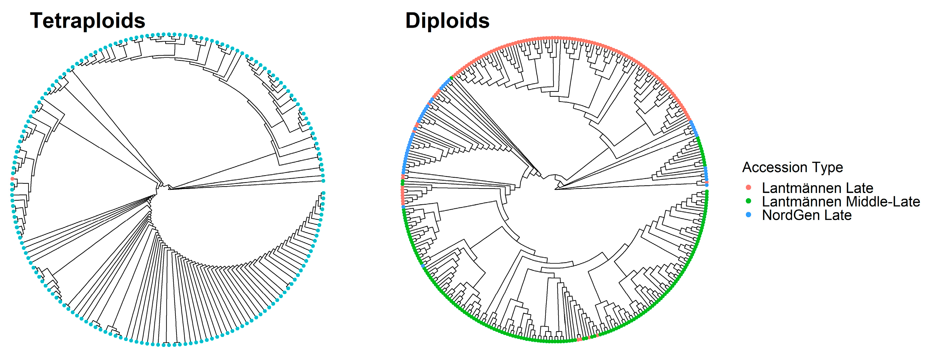
3.2. Genetic Diversity of Accessions

Neighbor-joining cluster analysis based on Nei’s standard genetic distance showed separation, with some overlaps, between the late and middle-late diploids with a slight population structure within each maturity group (Figure 5). The NordGen gene bank accessions were treated as late diploids in this study. However, some of them were closely clustered with Lantmännen’s middle-late diploids, suggesting that they are genetically more similar to the middle-late diploids. Additionally, some of the late diploids were clustered together with the middle-late diploids. This indicates that, even though they were bred as late diploids, they were genetically more similar to middle-late diploids, probably because of the exchange of germplasm between breeding programs. Compared with the diploids, the tetraploids showed a weak population structure. Nevertheless, they formed two major clusters, showing that some tetraploids had more genetic similarities to each other.

3.3. Model Reliability and Predictive Ability

For the forage quality traits, the ST_L model showed high broad-sense heritability (H²) ranging from 0.65 to 1 followed by MT₁ (0.37 to 1) and MT₂ (0.36 to 1) (Figure 6). The ST model had a 0.35–0.92 heritability range (Figure 6). The trait with the highest H² values in the ST model was yield. The H² from the ST model for the forage quality traits had a narrow range (all below 0.5) with the lowest in the tetraploids and highest in the late diploids. The MT₁ model had the highest H² values for the quality traits and lowest for yield, in which the H² of yield was affected differently by different quality traits and the cuts. For forage quality traits, there was little effect of cuts on H² in the ST and MT₁ models. H² varied between cuts in the case of the ST_L and MT₂ models. The MT₂ model performed well when there were high genetic correlations between traits. An example of this is the case of the middle-late diploid 2021 cut2. Here, the genetic correlations were 0.7 between NDF and yield, −0.8 between NDF and NEL, and −0.9 between NDF and protein content. The overall predictive ability was 0.56, 0.57, 0.58, and 0.56 for MT₁, ST_L, ST, and MT₂, respectively. The ST model had good predictive ability for many traits but not always, outperforming the MT₁ and MT₂ models for genetically non-correlated traits. Overall, none of the models had the best predictive ability across all germplasm subsets, traits, and cuts.

The success of the models seemed to be based on both the genetic correlation of traits and the BLUE variation. For example, the BLUEs of NEL ranged from 6 to 6.8 (Figure 2), and the predictive ability of the models was the lowest, on average, for this trait (Figure 7). For the late diploids, the MT₁ model outperformed the ST model in predicting NEL in the cut2 2021, although the correlation between NEL and yield was only 0.2. The ST_L model, on average, performed better at predicting yields in the middle-late diploids than in the late diploids and tetraploids. Nevertheless, the tetraploids had a higher overall genetic correlation between yield and cuts, where six corresponding measurements were weakly correlated (≥0.2) compared with 16 measurements in the middle-late subset.

The coefficients of determination (R²) between H² and the estimates of the models’ predictive abilities (Figure 8) indicate the extent to which the predictions were based on genetic variance. A low R² between the two suggests that BLUP variability is not mainly due to genotypic variance. However, if an increase in H² results in a higher predictive ability of a model, it shows that genotypic variance makes a major contribution to the variance in BLUPs. For forage quality traits, there seemed to be a decrease in PA as H² increased. The MT₁ model’s high H² could be due to a strong genetic correlation between traits where the interaction effect of genotypes and traits was overestimated. In the case of the ST model for quality traits, H² differed among the germplasm subsets, where the late diploids had the highest H² followed by the middle-late diploids and then the tetraploids. The reverse was observed for PA. This could be due to non-additive effects not explained by the Gaussian kernel. The ST_L and MT₂ models followed the hypothesis of increased H² as a function of predictability. The ST_L models could capture the non-additive effects in the interactions between genotype and cut, thus improving predictive ability as H² increased. The genetic correlations between forage quality traits (−0.4 to −0.8 between NEL and NDF, −0.5 to −0.9 between NDF and protein, and 0 to 0.7 between NEL and protein content) were stronger than between yield and forage quality traits (−0.4 to 0.7 between NDF and yield, −0.6 to 0.2 between NEL and yield, and −0.7 to 0.5 between protein and yield). Thus, the MT2 model performed better than the MT1 model because there was a stronger correlation between forage quality traits than between yield and forage quality traits. For yield, all multivariate models seemed to overestimate either PA or H², suggesting there was no beneficial model for improving yield when combined with quality. Overall, the variance in each correlation was high. This suggests that independent model formulation is needed based on each data set.

4. Discussion

4.1. Genotype and Phenotype Data

A key aspect of this study showcases the ability to use population-wide measurements of genotypes and phenotypes in genomic prediction. The phenotypic values of the accessions sown in plots, as is performed in a phenotype-based breeding program, were collected and analyzed. For genotyping, the development of pool-seq techniques is key to implementing GS methods in population-based red clover breeding. This is because genotyping an adequate number of individuals to represent each population is both costly and labor-intensive. Since the marker sets were different for tetraploids and diploids, genetic diversity analysis was performed separately. Osterman et al. [9,10] showed a modest population structure separating tetraploids from diploids. In this study, the results showed a very low population structure within each data set.

The BLUEs of each trait showed a non-linear trend over time (Figure 2), which indicates differences in growing conditions between the different cuts. Additionally, the correlations between traits within each data set differed across cuts, indicating that plant vigor and forage quality traits were unstable across the growing seasons.

The major difference between the late diploids and the other two germplasm subsets was the ratio between NEL, protein content, NDF, and yield (Figure 2). The late diploids had positive correlations between protein content, NEL, and yield while the reverse was observed for the middle-late diploids and tetraploids. This could be the effect of cultivation conditions as the late and middle-late diploids were grown at different sites with different harvesting time points. It could also be a result of differences in the genotypes’ genetic makeups as there was a separation between the late and middle-late diploids when observing the population structure in the NJ tree generated based on Nei’s genetic distance.

4.2. Trial Design and BLUEs

The trial design used to collect phenotypic data was an augmented design at two and three locations for diploids and tetraploids, respectively. The motivation for using an augmented design was the cost–benefit, i.e., more accessions can be tested within a location. Northern Europe has the disadvantage of having few and small field trial sites; hence, an augmented design was a reasonable choice. Each trial was divided into four blocks containing 44 non-replicated treatments and two checks replicated 16 times each. The key to an augmented design is the use of checks replicated within the environment to model spatial variability, and between environments to explain the reaction norm [35]. Unfortunately, the specific parameters of the augmented design were not optimal for red clover, as accessions had higher phenotypic plasticity within the trial than expected. Hence, the measurements of each accession in the two or three trial sites needed to be combined to estimate the BLUEs. To estimate the effect of G $\times$ E interactions in future studies, increasing the number of checks is recommended so that they have adequate and uniform coverage of the trial site.

4.3. Correlations Between Traits and Their Effect on Predictability and Reliability

To increase predictive ability using a multi-trait or longitudinal model, the traits or cuts need to be correlated with one another. The model borrows information about the variation explained by the genotype in different traits or cuts, thereby increasing reliability and consequently predictive ability. This study showed increased predictive ability for correlations stronger than 0.5. Additionally, this study showed that the stronger the genetic correlation between traits, the more linear the relationship between reliability and predictive ability (Figure 8). This could be because genetic effects were better explained when genotype $\times$ trait was included in the model. By using the Gaussian kernel as a genetic relationship matrix, additive genetic effects were better explained. Nevertheless, it is worthwhile to consider non-additive effects in crops such as red clover that have high heterozygosity and suffer from inbreeding depression.

To predict forage quality traits, the Gaussian kernel was not enough. However, by including multiple traits with positive or negative genetic correlations higher than 0.5, genetic effects could be better captured (Figure 3 and Figure 7). Nonetheless, the predictive ability of the MT₂ model for some cuts was high for yield in the tetraploids and middle-late diploids and low for NDF in the same subsets compared with H². Hence, introducing multiple traits resulted in unaccounted additional effects. Although the use of multiple traits aided the model’s ability to explain the quality traits, it added complexity that affected the model’s ability to explain forage yield.

Multiple strong correlations (>±0.5) were found between traits (Figure 4B) and between cuts when measuring yield (Figure 4C). However, when the data were divided into subsets, two prominent correlation patterns were found between yield and quality traits (Figure 4A). The first pattern was a positive correlation between yield and NDF, which, in turn, were negatively correlated with protein content and NEL. This result suggests that the plants had denser and tougher stems and fewer leaves. The second pattern was the opposite, where positive correlations were observed between yield and the two quality parameters, protein content and NEL, which, in turn, were negatively correlated with NDF. This suggests that the plants had more leaves and fewer or finer stems [36]. The first pattern was prominent in the tetraploid accessions as well as in the middle-late diploids’ second and third cuts. The middle-late diploids’ first cut as well as all cuts of the late diploids showed the second pattern. This could be due to the plants’ maturity levels because younger plants with fine and delicate stems with more leaves are expected to show the second pattern [21]. This is possibly the case for the first cut of the middle-late diploids. However, with the colder and shorter growing seasons in northern Sweden, red clover is expected to be less mature at harvest; hence, the protein and NEL content could be higher. Another plausible explanation could be higher levels of rhizobacteria in the soil in northern Sweden [37], which would benefit protein synthesis due to the increased availability of bio-available nitrogen. However, this hypothesis needs to be analyzed through a multi-environment field trial with sites varying in levels of rhizobacteria.

As shown by Nay et al. [17], red clover cultivated in the northern region is adapted to the region’s specific growth conditions where it outperforms accessions adapted to the southern region because of its later maturity as well as vigor. Thus, the difference in growth patterns is probably due to a combination of genetic and environmental differences. Since multiple genes regulate the target traits, trait expression may differ between the germplasm subsets, as their breeding programs may have different goals. Support for this was observed in the correlation between PA and H², where the relationship between the two differed for each data set. It may be possible to capture these differences in growth patterns by utilizing ST_L models. Further development of the ST_L models could include data from additional years, especially for the quality traits. With an equal amount of data points for quality and yield, a multi-trait longitudinal model could be evaluated. However, with the increase in model complexity, more accessions are needed.

Longitudinal traits are often measured as growth or responses to biotic or abiotic stresses, where non-destructive phenotyping methods are preferred. Longitudinal models have been successful, for example, in dairy cows [38] and rice [39]. Hence, it could be interesting to apply non-destructive measures of dry matter yield and quality traits using near-infrared indices from drone imaging. With the increase in data points, Legendre polynomials or B-splines could be used to measure the relationship between maturity and the target traits. However, that would reframe the research question from a test of vigor and quality as a response to the stress of cutting to a question of growing rate and maturity. With more research on drone imaging for red clover to estimate yield and quality, nonlinear models can be compared to these models in the future.

As for the MT₂ model, the correlation between yield and multiple forage quality traits could be used to decrease the number of accessions sampled for forage quality analysis. As shown by Cuevas et al. [24], multi-trait models can be used to predict expensive traits using their genetic correlation with cheaper traits. To implement such a model, the ratio between predictive ability and missing data points of quality traits needs to be investigated to see if it is economically viable to use in breeding.

5. Conclusions

The analysis presented in this study provides valuable insights into the genotypic and phenotypic landscape of red clover, offering a solid foundation for future breeding efforts. By applying pooled sequencing methods, a large number of high-quality SNP markers were obtained, facilitating genetic diversity studies and genomic prediction. The observed trends in genetic values for biomass yield and quality traits underscore the complexity of trait dynamics over time and across germplasm subsets. Notably, correlations between traits and their implications for the models’ predictive abilities and reliabilities highlight the importance of considering genetic correlations in multi-trait models. Overall, this study advances our understanding of red clover genetics. It also sets the stage for more targeted and efficient breeding strategies to enhance yield and quality traits in this agriculturally significant crop.

References

1. Smith, R.R.; Taylor, N.L.; Bowley, S.R. Red Clover. In Clover Science and Technology; John Wiley & Sons, Ltd.: Hoboken, NJ, USA, 1985; pp. 457–470. ISBN 978-0-89118-218-4. [Google Scholar]
2. Taylor, N.L.; Quesenberry, K.H. Historical Perspectives. In Red Clover Science; Taylor, N.L., Quesenberry, K.H., Eds.; Current Plant Science and Biotechnology in Agriculture; Springer: Dordrecht, The Netherlands, 1996; pp. 1–10. ISBN 978-94-015-8692-4. [Google Scholar]
3. Sato, S.; Isobe, S.; Asamizu, E.; Ohmido, N.; Kataoka, R.; Nakamura, Y.; Kaneko, T.; Sakurai, N.; Okumura, K.; Klimenko, I.; et al. Comprehensive Structural Analysis of the Genome of Red Clover (Trifolium pratense L.). DNA Res. 2005, 12, 301–364. [Google Scholar] [CrossRef] [PubMed]
4. Taylor, N.L.; Quesenberry, K.H. Tetraploid Red Clover. In Red Clover Science; Taylor, N.L., Quesenberry, K.H., Eds.; Current Plant Science and Biotechnology in Agriculture; Springer: Dordrecht, The Netherlands, 1996; pp. 161–169. ISBN 978-94-015-8692-4. [Google Scholar]
5. Taylor, N.L.; Giri, N. Frequency and Stability of Tetraploids from 2X–4X Crosses in Red Clover1. Crop Sci. 1983, 23, 1191–1194. [Google Scholar] [CrossRef]
6. Öhberg, H. Studies of the Persistence of Red Clover Cultivars in Sweden. 2008. Available online: https://pub.epsilon.slu.se/1741/ (accessed on 7 July 2021).
7. Amdahl, H.; Aamlid, T.S.; Ergon, Å.; Kovi, M.R.; Marum, P.; Alsheikh, M.; Rognli, O.A. Seed Yield of Norwegian and Swedish Tetraploid Red Clover (Trifolium pratense L.) Populations. Crop Sci. 2016, 56, 603–612. [Google Scholar] [CrossRef]
8. Zanotto, S.; Palmé, A.; Helgadóttir, Á.; Daugstad, K.; Isolahti, M.; Öhlund, L.; Marum, P.; Moen, M.A.; Veteläinen, M.; Rognli, O.A.; et al. Trait Characterization of Genetic Resources Reveals Useful Variation for the Improvement of Cultivated Nordic Red Clover. J. Agron. Crop Sci. 2021, 207, 492–503. [Google Scholar] [CrossRef]
9. Osterman, J.; Hammenhag, C.; Ortiz, R.; Geleta, M. Insights into the Genetic Diversity of Nordic Red Clover (Trifolium pratense) Revealed by SeqSNP-Based Genic Markers. Front. Plant Sci. 2021, 12, 2402. [Google Scholar] [CrossRef]
10. Osterman, J.; Hammenhag, C.; Ortiz, R.; Geleta, M. Discovering Candidate SNPs for Resilience Breeding of Red Clover. Front. Plant Sci. 2022, 13, 997860. [Google Scholar] [CrossRef] [PubMed]
11. Jordbruksaktuellt 23 år innan ny sort når Marknaden. Available online: https://www.ja.se/artikel/2226512/23-r-innan-ny-sort-nr-marknaden.html (accessed on 2 November 2020).
12. Meuwissen, T.H.E.; Hayes, B.J.; Goddard, M.E. Prediction of Total Genetic Value Using Genome-Wide Dense Marker Maps. Genetics 2001, 157, 1819–1829. [Google Scholar] [CrossRef]
13. Hayes, B.J.; Cogan, N.O.I.; Pembleton, L.W.; Goddard, M.E.; Wang, J.; Spangenberg, G.C.; Forster, J.W. Prospects for Genomic Selection in Forage Plant Species. Plant Breed. 2013, 132, 133–143. [Google Scholar] [CrossRef]
14. Taylor, N.L.; Quesenberry, K.H. Reproductive Biology, Genetics and Evolution. In Red Clover Science; Taylor, N.L., Quesenberry, K.H., Eds.; Current Plant Science and Biotechnology in Agriculture; Springer: Dordrecht, The Netherlands, 1996; pp. 25–43. ISBN 978-94-015-8692-4. [Google Scholar]
15. Futschik, A.; Schlötterer, C. The Next Generation of Molecular Markers from Massively Parallel Sequencing of Pooled DNA Samples. Genetics 2010, 186, 207–218. [Google Scholar] [CrossRef]
16. Frey, L.A.; Vleugels, T.; Ruttink, T.; Schubiger, F.X.; Pegard, M.; Skøt, L.; Grieder, C.; Studer, B.; Roldán-Ruiz, I.; Kölliker, R. Phenotypic Variation and Quantitative Trait Loci for Resistance to Southern Anthracnose and Clover Rot in Red Clover. Theor. Appl. Genet. 2022, 135, 4337–4349. [Google Scholar] [CrossRef]
17. Nay, M.M.; Grieder, C.; Frey, L.A.; Amdahl, H.; Radovic, J.; Jaluvka, L.; Palmé, A.; Skøt, L.; Ruttink, T.; Kölliker, R. Multi-Location Trials and Population-Based Genotyping Reveal High Diversity and Adaptation to Breeding Environments in a Large Collection of Red Clover. Front. Plant Sci. 2023, 14, 1128823. [Google Scholar] [CrossRef] [PubMed]
18. Fè, D.; Cericola, F.; Byrne, S.; Lenk, I.; Ashraf, B.H.; Pedersen, M.G.; Roulund, N.; Asp, T.; Janss, L.; Jensen, C.S.; et al. Genomic Dissection and Prediction of Heading Date in Perennial Ryegrass. BMC Genom. 2015, 16, 921. [Google Scholar] [CrossRef] [PubMed]
19. Skøt, L.; Nay, M.M.; Grieder, C.; Frey, L.A.; Pégard, M.; Öhlund, L.; Amdahl, H.; Radovic, J.; Jaluvka, L.; Palmé, A.; et al. Including marker x environment interactions improves genomic prediction in red clover (Trifolium pratense L.). Front. Plant Sci. 2024, 15, 1407609. [Google Scholar] [CrossRef] [PubMed]
20. Tucak, M.; Popović, S.; Čupić, T.; Španić, V.; Meglič, V. Variation in Yield, Forage Quality and Morphological Traits of Red Clover (Trifolium pratense L.) Breeding Populations and Cultivars. Zemdirb.-Agric. 2013, 100, 63–70. [Google Scholar] [CrossRef]
21. Abd El Moneim, A.M.; Khair, M.A.; Rihawi, S. Effect of Genotypes and Plant Maturity on Forage Quality of Certain Forage Legume Species Under Rainfed Conditions. J. Agron. Crop Sci. 1990, 164, 85–92. [Google Scholar] [CrossRef]
22. Falconer, D.S.; Mackay, T.F.C. Introduction to Quantitative Genetics, 4th ed.; Addison Wesley Longman: Harlow, UK, 1996. [Google Scholar]
23. Semagn, K.; Crossa, J.; Cuevas, J.; Iqbal, M.; Ciechanowska, I.; Henriquez, M.A.; Randhawa, H.; Beres, B.L.; Aboukhaddour, R.; McCallum, B.D.; et al. Comparison of Single-Trait and Multi-Trait Genomic Predictions on Agronomic and Disease Resistance Traits in Spring Wheat. Theor. Appl. Genet. 2022, 135, 2747–2767. [Google Scholar] [CrossRef]
24. Cuevas, J.; Reslow, F.; Crossa, J.; Ortiz, R. Modeling Genotype × Environment Interaction for Single and Multitrait Genomic Prediction in Potato (Solanum tuberosum L.). G3 Genes Genomes Genet. 2023, 13, jkac322. [Google Scholar] [CrossRef]
25. De Vega, J.J.; Ayling, S.; Hegarty, M.; Kudrna, D.; Goicoechea, J.L.; Ergon, Å.; Rognli, O.A.; Jones, C.; Swain, M.; Geurts, R.; et al. Red Clover (Trifolium pratense L.) Draft Genome Provides a Platform for Trait Improvement. Sci. Rep. 2015, 5, 17394. [Google Scholar] [CrossRef]
26. Li, H.; Durbin, R. Fast and accurate short read alignment with Burrows-Wheeler Transform. Bioinformatics 2009, 25, 1754–1760. [Google Scholar] [CrossRef]
27. Garrison, E.; Marth, G. Haplotype-based variant detection from short-read sequencing. arXiv 2012, arXiv:1207.3907. [Google Scholar]
28. Empfehlungen zur Energie und Nährstoffversorgung der Milchkühe und Aufzuchtrinder; DLG Verlag: Frankfurt, Germany, 2001; Available online: https://www.dlg-verlag.de/shop/empfehlungen-zur-energie-und-nahrstoffversorgung-von-milchkuhen.html (accessed on 30 March 2024).
29. Van Soest, P.J.; Robertson, J.B.; Lewis, B.A. Methods for dietary fiber, neutral detergent fiber, and nonstarch polysaccharides in relation to animal nutrition. J. Dairy Sci. 1991, 74, 3583–3597. [Google Scholar] [CrossRef] [PubMed]
30. R Core Team. R: A Language and Environment for Statistical Computing; R Foundation for Statistical Computing: Vienna, Austria, 2013. [Google Scholar]
31. Jombart, T. Adegenet: A R Package for the Multivariate Analysis of Genetic Markers. Bioinformatics 2008, 24, 1403–1405. [Google Scholar] [CrossRef] [PubMed]
32. Yu, G.; Smith, D.K.; Zhu, H.; Guan, Y.; Lam, T.T.-Y. Ggtree: An r Package for Visualization and Annotation of Phylogenetic Trees with Their Covariates and Other Associated Data. Methods Ecol. Evol. 2017, 8, 28–36. [Google Scholar] [CrossRef]
33. Gu, Z.; Eils, R.; Schlesner, M. Complex Heatmaps Reveal Patterns and Correlations in Multidimensional Genomic Data. Bioinformatics 2016, 32, 2847–2849. [Google Scholar] [CrossRef]
34. Cullis, B.R.; Smith, A.B.; Coombes, N.E. On the design of early generation variety trials with correlated data. J. Agric. Biol. Environ. Stat. 2006, 11, 381–393. [Google Scholar] [CrossRef]
35. Moehring, J.; Williams, E.R.; Piepho, H.-P. Efficiency of Augmented P-Rep Designs in Multi-Environmental Trials. Theor. Appl. Genet. 2014, 127, 1049–1060. [Google Scholar] [CrossRef]
36. Leto, J.; Knežević, M.; Bošnjak, K.; Maćešić, D.; Štafa, Z.; Kozumplik, V. Yield and Forage Quality of Red Clover (Trifolium pratense L.) Cultivars in the Lowland and the Mountain Regions. Plant Soil Environ. 2004, 50, 391–396. [Google Scholar] [CrossRef]
37. Jambagi, S.; Hodén, K.P.; Öhlund, L.; Dixelius, C. Red Clover Root-Associated Microbiota Is Shaped by Geographic Location and Choice of Farming System. J. Appl. Microbiol. 2023, 134, lxad067. [Google Scholar] [CrossRef]
38. Bohmanova, J.; Miglior, F.; Jamrozik, J.; Misztal, I.; Sullivan, P.G. Comparison of Random Regression Models with Legendre Polynomials and Linear Splines for Production Traits and Somatic Cell Score of Canadian Holstein Cows. J. Dairy Sci. 2008, 91, 3627–3638. [Google Scholar] [CrossRef]
39. Campbell, M.; Momen, M.; Walia, H.; Morota, G. Leveraging Breeding Values Obtained from Random Regression Models for Genetic Inference of Longitudinal Traits. Plant Genome 2019, 12, 180075. [Google Scholar] [CrossRef]
Figure 1. A timeline of the cuts, where each time point is the harvest date of a cut. The points are colored based on the trial sites. Multiple points close together indicate that the harvest was conducted per block and spanned multiple days.
Agronomy 14 02445 g001
Figure 2. A violin plot of the estimated genetic values (BLUES) across the tested sites for (rows) net energy for lactation (NEL), neutral detergent fiber (NDF), protein content, and yield at each cut (columns) in the late diploids, middle-late diploids, and tetraploids. The mean is marked with a point on each violin.
Agronomy 14 02445 g002
Figure 3. A principal component analysis (PCA) on the corrected best linear unbiased estimators (BLUEs) across the tested sites for the 532 accessions, colored by germplasm subset (red for late diploids, green for middle-late diploids, and blue for tetraploids). The arrows show the loadings of each trait at each time point. The arrows are colored according to traits.
Agronomy 14 02445 g003
Figure 4. A heatmap (A) showing genetic correlations within traits (between cuts). The heatmap is split by subgroup and shows the Pearson correlation between dry matter yield (yield), protein, net energy for lactation (NEL), and neutral detergent fiber (NDF), arranged by cut (first, second, and third for 2021 and 2022). The Pearson correlations without consideration of subgroups between (B) traits and (C) cuts where each subgroup is separated by color. Each Pearson correlation is marked with asterisk signifying level of significance, where *** is p-value < 0.001.
Agronomy 14 02445 g004
Figure 5. Neighbor-joining trees based on Nei’s standard genetic distance for tetraploids (left) and diploids (right). Each terminal branch is an accession, which is color-labeled based on whether it is from NordGen or Lantmännen and either late- or middle-late-maturing.
Agronomy 14 02445 g005
Figure 6. Bar graphs showing model reliability calculated as H2 using the Cullis method for each cut. Each bar is colored according to single-trait (ST), single-trait-longitudinal (STL), multi-trait two traits (MT1), and multi-trait four traits (MT2). For MT1, the yield was modeled three times together with NDF, protein content, and NEL. The graphs are organized vertically according to traits and horizontally according to germplasm subsets.
Agronomy 14 02445 g006
Figure 7. Bar graphs of the predictive ability between the best linear unbiased estimators (BLUEs) and the mean best linear unbiased predictor (BLUP) of 100 iterations of 10-fold cross-validation for each trait and each cut of the three germplasm subsets. The bars are colored according to the model used to calculate the BLUPs. The graphs are organized vertically according to traits and horizontally according to germplasm subsets.
Agronomy 14 02445 g007
Figure 8. Predictive ability as a function of broad-sense heritability (H2) separated according to the models used. Each point is the result of a model on a specific trait in a specific subset. Each point has a shape according to the subset it belongs to and is colored by trait. The coefficient of determination (R2) was estimated from a linear regression of the predictive ability on H2. The black values are R2 values for all models across subsets and traits within each plot panel.
Agronomy 14 02445 g008
Disclaimer/Publisher’s Note: The statements, opinions and data contained in all publications are solely those of the individual author(s) and contributor(s) and not of MDPI and/or the editor(s). MDPI and/or the editor(s) disclaim responsibility for any injury to people or property resulting from any ideas, methods, instructions or products referred to in the content.