Abstract
In order to alleviate the shortage of water in Xinjiang cotton fields, to ensure the sustainable development of the cotton industry in southern Xinjiang, it is necessary to determine a suitable “dry sowing and wet emergence” water quantity plan for cotton fields in southern Xinjiang to change the current situation. In this study, to explore the irrigation regime of “dry sowing and wet emergence” for cotton in Korla, Xinjiang, by combining field experiments and modeling simulations, the effects of different irrigation amounts on the water–heat–salt and seedling emergence characteristics of “dry sowing and wet emergence” cotton fields were investigated; the soil, water, and salt transport under different irrigation regimes was simulated by using HYDRUS-2D, and the seedling emergence rate of the cotton under different irrigation regimes was obtained through the establishment of a regression model. The results indicated that, in the field experiment, the soil water content of the 0−40 cm soil layer showed an overall trend of first increasing and then decreasing with time, while the soil salt content showed an overall trend of first decreasing and then increasing over time. The soil water content at the drip heads and cotton rows position, as well as on the 15th day, increased by an average of 5.58 cm3·cm−3 compared to before irrigation, and the soil salt content decreased by an average of 2.74 g/kg compared to before irrigation. In the irrigation water range of 675−825 m3/hm2, reducing the irrigation water amount increased the cotton emergence rate by 3.86% and the cotton vigor index by 70.53%. After the model simulation, it is recommended to choose the cotton “dry sowing and wet emergence” irrigation regime with a low to medium water amount (300−450 m3/hm2) at 14-day intervals or a low to medium water amount (300−375 m3/hm2) at 7-day intervals, which can obtain a higher seedling emergence rate.
1. Introduction
Cotton, as a widely cultivated economic crop, has a significant impact on the global cotton market, especially the Chinese cotton market [1]. The current cotton industry has become a pillar industry for the development of the agricultural economy in the Xinjiang region [2]. In 2024, the cotton planting area in Xinjiang will reach 2.44 × 10⁶ hm2, accounting for 89.98% of the total cotton planting area in the country, with the cotton growing area in Bazhou amounting to 2 × 10⁵ hm2, accounting for 8.18% of the total planting area in the Xinjiang region.
The Xinjiang region is already facing severe challenges of water scarcity; however, with the expansion of arable land in Xinjiang and the necessary winter and spring irrigation before cotton sowing [3], the demand for water resources in Xinjiang’s cotton field industry has increased. Especially in the southern Xinjiang region, due to the arid climate, strong evaporation, and high soil salt, cotton requires more water for winter or spring irrigation, further exacerbating the water scarcity situation in the southern Xinjiang region. Therefore, to alleviate the shortage of regional water resources and ensure the sustainable development of the cotton field industry in southern Xinjiang, it is imperative to implement the “dry sowing and wet emergence” drip irrigation technology, similar to the practices in northern Xinjiang [4].
As a cotton planting technique utilizing drip water under film for moisture retention and salt leaching, the “dry sowing and wet emergence” technology changed the traditional practice of irrigating before sowing. Instead, it meets the germination requirements of seeds by applying a small amount of water post-sowing [5]. This model has the significant advantages of saving water resources, improving cotton emergence rates, promoting cotton yield, and income increase [6], and it has high promotion value [7].
At present, this technique has been widely applied in the machine-harvested cotton planting model of “one film, three tubes, six rows” in northern Xinjiang. However, in the Korla area of southern Xinjiang, the promotion of the “dry sowing and wet emergence” technology has been limited, due to seedling shortage and death in severely saline–alkali land [5]. Moreover, the machine-harvested cotton planting pattern in this area was mostly one film, three tubes, and three rows. Compared to the one film, three tubes, and six rows planting pattern, the “one film, three tubes, three rows” planting pattern exhibited advantages in terms of the cotton plant height and the initial node height of fruit branches, while maintaining a higher leaf area index and achieving relatively higher yields [8]. Therefore, it is essential to explore the irrigation regime of the “dry sowing and wet emergence” technique under the “one film, three tubes, three rows” planting pattern in the Korla region to validate the application effect of this technology in southern Xinjiang.
At present, there have been many studies on the technology of “dry sowing and wet emergence” in cotton fields. For example, Zheng Ming et al. [9] showed that in cotton planting when the irrigation frequency was twice and the irrigation amounts were 675 m3/hm2 and 225 m3/hm2, respectively, the cotton exhibited the highest emergence rate and the lowest soil harden degree, and the cotton diameter and plant height were better than with other treatments. Shao Jingjing et al. [10] found through soil box experiments that although the “dry sowing and wet emergence” technique can improve the cotton seedling emergence rate, when the soil salt content was higher than 4.03 g/kg the growth of the cotton was significantly inhibited and the critical value of salt stress was determined. The study by Dong Xin et al. [11] revealed that double film cover has the strongest water retention capacity, can significantly prevent the surface accumulation of soil salt, and has the best thermal insulation effect; as a result, it is more conducive to improving the emergence rate and yield of cotton. Ding Yu et al. [12] further explored double film cover conditions and found that the optimal treatment for water saving and seedling protection was an irrigation amount of 675 m3/hm2 and an irrigation frequency of once.
The previous studies on the “dry sowing and wet emergence” irrigation pattern, mentioned above, mainly focused on the surrounding areas of Shaya County, Aksu City, and the cotton planting pattern of one film, three tubes, and six rows was commonly used. However, these studies were limited in the setting of the water amounts, resulting in certain limitations in the universality and depth of the research conclusions.
At present, the “dry sowing and wet emergence” technology has not been widely popularized in the Korla area of southern Xinjiang, given the unique planting pattern of one film, three tubes, and three rows. The exploration of the relationship between the cotton emergence rate and soil water, heat, and salt under the “dry sowing and wet emergence” treatment is slightly insufficient, and further systematic research is needed to determine the “dry sowing and wet emergence” water amounts scheme for the planting pattern of one film, three tubes, and three rows. Therefore, this study selected the cotton variety “Xinlu Zhong 55” as the experimental object, adopted the planting pattern of one film, three tubes, and three rows, and set up three different irrigation amounts treatments to compare and analyze the effects of each treatment on the soil water–heat–salt, growth indicators, and emergence rate in cotton fields. The HYDRUS-2D 2.04 version numerical simulation software was used to calibrate and validate the model using measured water–salt data. Through the model simulation, this study explored the dynamic changes in soil water and salt during the cotton seedling emergence period under different “dry sowing and wet emergence” irrigation regimes, and a regression model between the soil water–salt change and cotton seedling emergence rate was established. Finally, based on the model scenario prediction, the optimal irrigation regime of “dry sowing and wet emergence” under the cotton planting pattern of “one film, three tubes, three rows” was selected. This provides a reference basis for alleviating the shortage of water resources in the cotton fields in the Korla area and also provides new ideas and methods for the development of cotton planting technology in the future.
2. Materials and Methods
2.1. Overview of the Study Area
The experimental site is located in Company 10, 29th Regiment in Korla City, Xinjiang, characterized by drought and low rainfall, and belongs to a temperate continental arid climate. The annual average temperature is 11.4 °C, the annual average rainfall is 58.6 mm, the annual average evaporation is 2700 mm, the annual sunshine duration is 2990 h, and the annual total radiation reaches 6000 mJ/m2. The soil texture is sandy loam, with an average pH of 8.13 and an average soil salt content of 13.39 g/kg at a depth of 0−40 cm, belonging to severe saline–alkali soil. The basic physical and chemical properties of the soil in the experimental site are shown in Table 1, using the ring knife method [13] to determine the soil bulk density, saturated water content, and field water holding capacity, using a LS 13 320 laser particle size analyzer (Beckman Coulter Trading Co., Ltd., Shanghai, China) to determine the soil particle size composition. The Tianqi Intelligent Ecological Station (INSENTEK Oriental Zhigan Co., Ltd., Hangzhou, China) installed in the experimental area can automatically record meteorological data such as precipitation, air temperature, and relative humidity every hour, and the meteorological data are shown in Figure 1.

Table 1.
Basic physical properties of the soil.
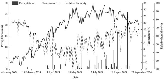
Figure 1.
Meteorological data chart.
2.2. Experimental Design
The cotton variety was “Xinluzhong 55”, and the sowing time was 12 April 2024. The “dry sowing and wet emergence” drip time was April 16. The research stage of this experiment was the cotton emergence period (18 April 2024−1 May 2024). The cotton adopted the planting pattern of one film, three tubes, and three rows, and had the unified use of mechanical mulching, a film width of 2.05 m, a film thickness of 0.02 mm, a film spacing of 50 cm, a cotton spacing of 10 cm, and a sowing depth of 1−2 cm. The irrigation water source was canal water, and the irrigation water mineralization was 0.52 g/L; using a single-wing labyrinth drip irrigation belt, the drip head flow rate was 2.1 L/h, and the drip head spacing was 20 cm.
The experiment set three different amounts of irrigation water treatment, respectively, 525 m3/hm2 (T1 treatment), 675 m3/hm2 (T2 treatment), and 825 m3/hm2 (T3 treatment); a 20 mm rotary-wing water meter was used for the water measurement. Each treatment zone had a width of one membrane and a length of 15 m. Three sets of repetitions were set up, and a protective row was set up between adjacent zones. The cotton planting pattern is shown in Figure 2. The experimental layout plan is shown in Figure 3.
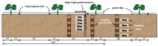
Figure 2.
Cotton planting pattern (unit: cm).
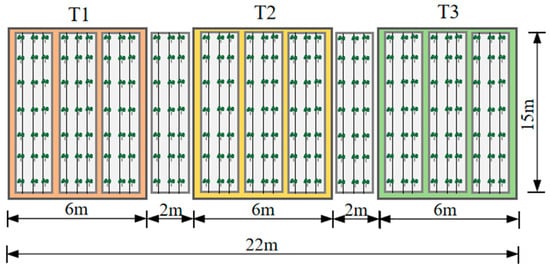
Figure 3.
Layout plan.
2.3. Measurement Indicators
2.3.1. Soil Water Content
Soil samples were collected between two drip irrigation belts, between drip heads and cotton rows, and between the bare ground at the same profile of different treatment plots using soil auger. The collection time was before the start of irrigation and on the 1st, 5th, 10th, and 15th days after the start of irrigation. Respectively, the depth of the soil samples being collected were in one layer of every 10 cm, to a depth of 40 cm. The drying method [14] refers to placing the collected soil sample in an oven at 105 °C for 6−8 h to dry and then obtaining the dry soil mass by weighing. The drying method was utilized to determine the mass water content of the sandy loam soil (soil particle size < 2 mm), which was multiplied by the volumetric weight of the corresponding soil layer to obtain the volumetric soil water content, and the final result was averaged.
2.3.2. Soil Salt Content
Assuming the measured salt sample was consistent with the soil water sample, the collected soil samples were naturally air-dried and sieved through a 2 mm sieve, and 10 g of air-dried soil sample was weighed and mixed with 50 mL of distilled water in a ratio of 1:5. After standing for 24 h, the conductivity of the filtrate was measured using an MP515−03 high concentration conductivity meter, and the reuse regression equation [15] was used to calculate the soil salinity:
where S is the soil salt content, g/kg; and COND is the conductivity, mS/cm.
S = 0.2564 × COND + 0.1446
2.3.3. Soil Temperature
Maintaining an appropriate soil temperature is also one of the important factors affecting the germination rate of cotton. Research has shown that at suitable growth temperatures, higher temperatures are more favorable for the germination and emergence of cotton seeds [16]. Therefore, obtaining soil temperature data is indispensable.
Five right-angle ground thermometers were inserted near the cotton seedlings in each treatment and observed the daily temperature changes at 5 cm, 10 cm, 15 cm, 20 cm, and 25 cm below the surface of the ground; the observation time was from 11:30 to 12:00 every day.
The formula for the soil effective accumulated temperature is as follows:
where K is the total effective accumulated temperature required for cotton seedling emergence, °C; N is the number of days required for cotton from sowing to seedling emergence, days; T is the average temperature of the day, °C; and C is the minimum temperature of 14 °C for cotton growth and development.
K = N × (T − C)
2.3.4. Characteristics of Cotton Emergence
At the end of irrigation, the emergence of seedlings in each treatment plot was counted at 12:00 am every day, and the daily emergence rate of each treatment plot was recorded every day. The observation continued until 15 days after irrigation; see reference [17] for the correlation formula between the seedling emergence rate and seedling vigor index. After the cotyledon leaves of the cotton seedlings had unfolded, 15 cotton seedlings with consistent growth were selected from each treatment plot, and the heights of the seedlings were determined using a tape measure.
The formula for the seedling emergence rate is as follows:
where ER is the cotton emergence rate, %; NSE is the number of seedlings, plants; and CH is the total number of cotton holes, plants.
The formula for the seedling emergence vigor index is as follows:
where EI is the emergence index; NSEn is the number of seeds emerging in n days, plants; and n is the number of days.
2.4. Model Simulation
2.4.1. Cotton Emergence Process—Logistic Modeling
The LOGISTIC model [18] was used to describe the cotton emergence process with the following equation:
where Y is the seedling emergence rate, %; K is the maximum emergence rate, %; t is the number of days after sowing, days; and a and b are the empirical coefficients.
2.4.2. HYDRUS-2D Model
HYDRUS-2D [19] is a two-dimensional numerical simulation software for the movement of water, heat, and various solutes in porous media, developed by the National Saline Soil Improvement Center in the United States.
- 1.
- Soil water transport equation
Assuming the soil is homogeneous in all respects and the soil texture is uniformly distributed, ignoring the soil moisture hysteresis effect, and not considering the influence of the solute potential and temperature potential on water transport, the process of soil water movement can be described by the equation of Richards [20] in accordance with the treatment of axisymmetric problems:
where ψ is the total water potential, MPa; K(θ) is the unsaturated soil hydraulic conductivity, cm/d; θ is the soil volumetric water content, cm3/cm3; t is the water transport time, days; and x and z are the two-dimensional spatial coordinates, cm.
- 2.
- Soil solute transport equation
Soil solute transport obeys the law of conservation of mass and the continuum equation, and the model was described by the convective dispersion equation for soil solute transport [21]:
where θ is the soil volumetric water content, cm3/cm3; c is the solute concentration in the dissolved state, g/cm3; DT is the lateral dispersion coefficient, cm2/d; DL is the longitudinal dispersion coefficient, cm2/d; q is the soil water flow flux, cm/d; t is the water transport time, days; and x and z are the two-dimensional spatial coordinates, cm.
- 3.
- Basic equation of soil evapotranspiration
The Penman–Monteith [22] formula, used to estimate the daily reference crop evapotranspiration and transpiration, is as follows:
where ET0 is the reference crop evapotranspiration, mm; Rn is the net radiation in the field, MJ/(m2·d); G is the soil heat flux, MJ/(m2·d); T is the daily average air temperature, °C; γ is the thermometer constant, KPa/°C; µ2 is the average wind speed at a certain height, m/s; es is the saturated water vapor pressure, KPa; ea is the actual water vapor pressure, KPa; and Δ is the slope of the saturated vapor pressure curve, KPa/°C.
- 4.
- Initial and boundary conditions for soil water movement
Taking the 0−50 cm soil profile as the research object, a two-dimensional model simulation area was established (Figure 4); the horizontal length of the simulation area was 285 cm (the width of one plastic film + the width of two bare lands between the films), and the vertical depth was 50 cm. The grid refinement of the unit at the drip head position was performed, and observation points were set at the corresponding locations of the model according to the actual measured points to ensure that the simulated points of the simulated values were consistent with the actual sampling points of the measured values.
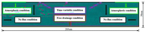
Figure 4.
Schematic diagram of the simulation area.
In the upper boundary conditions of the model simulation area, the covered portion is the zero flux boundary, the uncovered portion is the atmospheric boundary, and the drip head position is the variable flux boundary. The lower boundary condition is a free drainage boundary; the left and right boundary conditions are zero flux boundaries.
Initial condition:
Boundary condition:
Upper boundary condition (covered with film):
Upper boundary condition (uncovered with film):
Lower boundary conditions:
Left and right boundary conditions:
where K(θ) is the unsaturated soil hydraulic conductivity, cm/d; θ is the soil volumetric water content, cm3/cm3; h is the negative pressure water head at the boundary, cm; q is the surface water flux, L/h; E is the soil surface evaporation intensity, cm/d; t is the water transport time, days; and x and z are the two-dimensional spatial coordinates, cm.
- 5.
- Initial and boundary conditions for soil salt transport
Initial condition:
Boundary condition:
Upper boundary condition (covered with film):
Upper boundary condition (uncovered with film):
Lower boundary conditions:
where c0 is the initial salt content, g/kg; q is the surface water flux, L/h; and cb is the salt content of the groundwater, g/kg.
- 6.
- Model mesh discretization
The discrete time unit of the simulation is the day, with a starting time of 0 days and an ending time of 15 days. The starting time step is 1 × 10⁻⁴ days, the minimum time step is 1 × 10⁻⁵ days, and the maximum time step is 5 days. Using time-varying boundary conditions, the whole simulation area is discretized by irregular triangle grids, with a grid node divided every 1 cm. The total number of nodes is 15,602, generating 31,202 triangular grids.
2.5. Evaluation of Model Results
The model accuracy was verified using the coefficient of determination (R2), root mean square error (RMSE), and mean absolute error (MAE), where the closer the value of R2 was to 1, the better the model fit was; the closer the values of RMSE and MAE were to 0, the higher the model accuracy was.
where n represents the number of total data; Oi represents the simulated values; Pi represents the measured value; represents the mean of the simulated values; and represents the mean of the measured values.
2.6. Data Processing
Microsoft Excel 2010 was used for data organization and calculation, Origin 2022 was used for graph drawing, and SPSS 26 was used for correlation analysis. The simulation of the soil moisture and salinity was conducted using HYDRUS-2D version 2.04, and the download link can be found in reference [23].
3. Result and Analysis
3.1. Effects of Different Water Amounts on Soil Water, Heat, and Salt Conditions and Seedling Growth
3.1.1. Characteristics of Soil Water Distribution
The changes in the soil water with the different water gradients are shown in Figure 5.
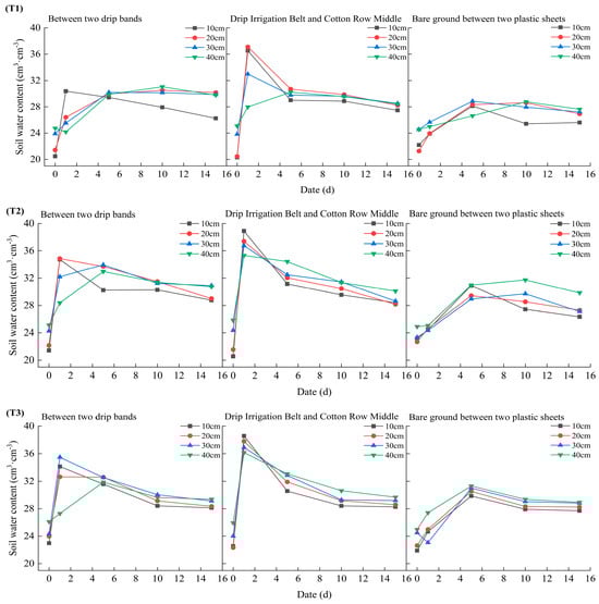
Figure 5.
Changes in the soil water content under the different water gradients. Note: the horizontal coordinate date refers to the date after the start of irrigation; T1, T2, and T3 represent the three treatments with the irrigation amounts of 525 m3/hm2, 675 m3/hm2, and 825 m3/hm2, respectively; each processed subgraph represents, from left to right, the changes in the soil water content between two drip bands, between drip irrigation belts and cotton rows, and between bare land positions in the film.
The variation pattern of the soil water content between two drip irrigation belts: After the end of irrigation, the soil water content in the 10−40 cm soil layer increased by varying degrees in the T1 treatment, and the increase gradually decreased with the depth of the soil layer. The increase in the soil water content in the 10 cm soil layer was 9.92 cm3·cm−3, and the increase in the soil water content in the 30 cm soil layer was 1.62 cm3·cm−3. The soil water content of the 20 cm soil layer of the T2 treatment was the largest after irrigation, which was 34.86 cm3·cm−3, and the soil water content of the 10−40 cm soil layer showed a trend of increasing and then decreasing over time. The variation pattern of the soil water content in the T3 treatment was basically consistent with that in the T2 treatment.
The variation pattern of the soil water content between drip heads and cotton rows: Under the different treatments, the soil water content in the 10−40 cm soil layer showed a trend of first increasing and then decreasing with the passage of time. After irrigation stopped, the soil water content of the T1 treatment reached its peak at 37.10 cm3·cm−3 in the 20 cm soil layer, the T2 treatment reached its peak at 38.89 cm3·cm−3 in the 10 cm soil layer, and the T3 treatment reached its peak at 38.58 cm3·cm−3 in the 10 cm soil layer. On the 15th day, the soil water content of the 10−40 cm soil layer increased with the depth of the soil layer.
The variation pattern of the soil water content in bare soil between membranes: The soil water content of each treatment in the soil layer of 10−40 cm in 0−5 days, except for the soil water content in the soil layer of 30 cm in the T3 treatment which showed a decreasing trend in the first day, showed an increasing trend with the passage of time. The soil water content in the soil layer of 10−40 cm in the T1 and T2 treatments showed no obvious pattern after the 5th day. The soil water content in the soil layer of 10−40 cm in the T3 treatment gradually decreased and tended to stabilize over time.
In summary, the soil water content of the 0−40 cm soil layer in the three treatments showed a trend of increasing first, then decreasing, and finally stabilizing over time. The change in the soil water content was most significant at the drip head and cotton row positions, while the change in soil water content was smallest at the bare land position between the membranes.
3.1.2. Characteristics of Soil Salt Distribution
The changes in the soil salt with the different water amounts are shown in Figure 6. The average soil salt content of the 10−40 cm soil layer before irrigation in the T1, T2, and T3 treatments was 14.31 g/kg, 12.38 g/kg, and 13.48 g/kg, respectively.
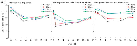
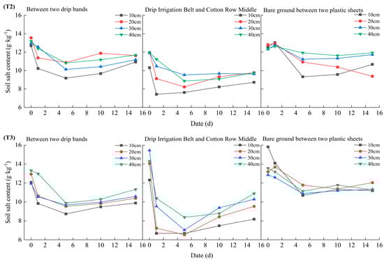
Figure 6.
Changes in the soil salt content under the different water gradients. Note: the horizontal coordinate date refers to the date after the start of irrigation; T1, T2, and T3 represent the three treatments with irrigation amounts of 525 m3/hm2, 675 m3/hm2, and 825 m3/hm2, respectively; each processed subgraph represents, from left to right, the changes in the soil salt content between two drip bands, between drip irrigation belts and cotton rows, and between bare land positions in the film.
The variation pattern of the soil salt content between two drip irrigation belts: Except for the T2 treatment, the soil salt content in the 20 cm soil layer showed a trend of first decreasing, then increasing, and then decreasing over time. The soil salt content in the 10−40 cm soil layer of the other treatments showed a trend of first decreasing and then increasing over time. On the 5th day, the soil salt content in the 10 cm soil layer of the T1, T2, and T3 treatments reached the lowest levels. On the 15th day, the soil salt content in the 40 cm soil layer of the T1, T2, and T3 treatments reached the highest levels, which were 12.88 g/kg, 11.68 g/kg, and 11.33 g/kg, respectively.
The variation pattern of the soil salt content between drip heads and cotton rows: The soil salt content in the 10−40 cm soil layer of each treatment showed a trend of first decreasing and then increasing over time, while the soil salt content in the 30 cm and 40 cm soil layers reached its lowest point on the fifth day after irrigation. With the increase in the irrigation amount, the soil salt content in the 10−40 cm soil layer gradually decreased. The average soil salt content in the 10−40 cm layer of the T1 treatment was between 10.63 and 14.00 g/kg at different times, the average soil salt content in the 10−40 cm layer of the T2 treatment was between 8.56 and 11.53 g/kg at different times, and the average soil salt content in the 10−40 cm layer of the T3 treatment was between 7.16 and 14.03 g/kg at different times.
The variation pattern of the soil salt content in bare soil between membranes: The T1 treatment had the lowest average soil salt content of 12.45 g/kg in the 10−40 cm layer on the 5th day, the T2 treatment had the lowest average soil salt content of 10.73 g/kg in the 10−40 cm layer on the 10th day, and the T3 treatment had the lowest average soil salt content of 11.12 g/kg in the 10−40 cm layer on the 5th day. Moreover, with the passage of time, the soil salt content in the 10−40 cm layer of each treatment showed a slow increasing trend.
In summary, the soil salt content of the 0−40 cm soil layer in the three treatments showed a trend of first decreasing and then increasing over time. Among them, the change in the soil salt content was most significant at the drip head and cotton row positions, and the change in the soil salt content was the smallest at the bare land position between the films.
3.1.3. Characteristics of Soil Temperature Changes
The changes in temperature over time for each treatment under the different water amounts are shown in Figure 7. The trend of the daily temperature changes with time for the different soil depths under each treatment was roughly the same, and the date with the largest increase in daily temperature within 14 days was 19 April, on which the average temperatures of each soil layer of the T1, T2, and T3 treatments had increased by 3.88 °C, 4.22 °C, and 4.00 °C, respectively, compared to 18 April. Starting from 26 April, the temperatures of the different soil layers in each treatment slightly decreased; in the T1, T2 and T3 treatments, the average temperature of each soil layer decreased by 1.39 °C, 1.71 °C, and 1.14 °C, respectively. In terms of the degree of change in the soil layer temperature, the temperature at the depth of the 5 cm soil layer had the greatest change, and the temperature at the depth of the 25 cm soil layer had the least change. Therefore, the amplitude of the soil temperature changes gradually decreases with the increase in the soil depth.
Figure 7.
Temperature changes under different water amounts. Note: The label (a) in the image represents the temperature change of the T1 treatment (irrigation amounts of 525 m3/hm2), The label (b) in the image represents the temperature change of the T2 treatment (irrigation amounts of 675 m3/hm2), The label (c) in the image represents the temperature change of the T3 treatment (irrigation amounts of 825 m3/hm2).
The changes in the average temperature and effective accumulated temperature at the different soil depths under the three treatments are shown in Figure 8. The average temperature and effective accumulated temperature of the three treatments at the depth of 5–15 cm are ranked as T2 > T3 > T1, while the average temperature and effective accumulated temperature of the three treatments at the depth of 20–25 cm are ranked as T1 > T2 > T3. This indicates a positive correlation between the soil average temperature and effective accumulated temperature. During the growth process of the cotton seedlings, the surface temperature was closely related to the emergence rate. The T2 treatment had a higher soil surface temperature compared to the other two treatments, providing a good growth environment for the subsequent cotton emergence.
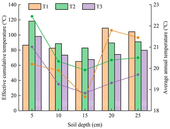
Figure 8.
Changes in effective accumulated temperature and average temperature under different water amounts. Note: The bar chart represents the effective accumulated temperature changes at different soil depths under different treatments, while the line chart represents the average ground temperature changes at different soil depths under different treatments.
3.1.4. Analysis of Cotton Emergence Situation
The variations in the daily emergence rate at the different water amounts are shown in Figure 9. With the increase in the number of days of emergence, the emergence rate of the cotton showed a gradually increasing trend and finally stabilized at 13 days. On the day of April 22, the emergence rates of all three treatments exceeded 50%. After that, the growth rate of the emergence rates of each treatment significantly slowed down, and the final emergence rates of the three treatments were T2 > T1 > T3. Compared to the T3 treatment, the rate of the emergence of the T1 treatment increased by 2%, and the rate of the emergence of the T2 treatment increased by 3.86%.
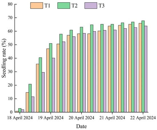
Figure 9.
Changes in seedling emergence rate under different water amounts.
The seedling emergence vigor indexes under the different water amounts are shown in Figure 10. The ranking of the seedling vigor index was T2 > T1 > T3. A variance analysis of the seedling vigor index of the three treatments showed there was no significant difference between the T1 and T2 treatments, but there was a significant difference between the T1 and T2 treatments and the T3 treatment. Compared to the T3 treatment, the seedling vigor index of the T1 treatment increased by 54.89%, and the seedling vigor index of the T2 treatment increased by 70.53%. Therefore, the appropriate reduction in the irrigation amount can moderately increase the seedling emergence rate and seedling vigor index of cotton seeds.
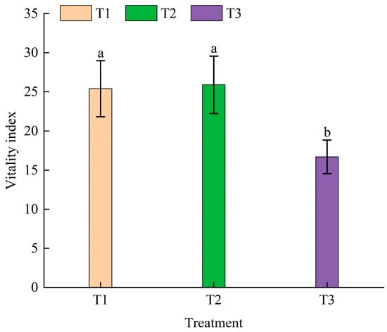
Figure 10.
Seedling emergence index under different water amounts. Note: The error bar represents the standard error. The differences between different treatments were determined through Duncan’s test of variance. The different letters above the bar chart indicate significant differences between treatments when p < 0.05.
The logistic fitting curves of the seedling emergence rates under the different water amounts are shown in Table 2. The determination coefficient R2 of the seedling emergence rate under the three different water gradients was greater than 0.960, the root mean square error RMSE was between 2.54% and 4.30%, and the average absolute error MAE was between 2.18% and 3.67%. By fitting the curve, it was found that, when the sowing days were less than 5 days, the measured seedling emergence rate was slightly higher than the germination rate of the fitting curve. When the sowing days were greater than 5 days, the measured seedling emergence rates were slightly less than the germination rate of the fitting curve. Therefore, the logistic equation can better reflect the emergence process of the cotton under the different irrigation treatments.
Table 2.
Cotton emergence logistic equation under different water amounts.
The changes in the cotton plant height under the different water amounts are shown in Figure 11. The average plant height of the cotton seedlings under the three treatments was T1 > T2 > T3, with the T1 treatment having an average plant height of 5.70 cm, the T2 treatment having an average plant height of 5.64 cm, and the T3 treatment having an average plant height of 5.63 cm. There were no significant differences in the average plant height under the three treatments.
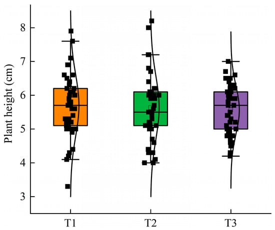
Figure 11.
Changes in seedling height under different water amounts.
3.1.5. Analysis of Factors Affecting Cotton Emergence Rate
The Pearson correlation analysis between the cotton emergence rate, soil water, heat, and salt, and seedling height is shown in Figure 12. Due to the fact that the shallow soil (0–20 cm) was a concentrated area for root systems during the early stages of sowing, the changes in soil water, heat, and salt in this layer were larger, which also has the greatest influence on the cotton seedling emergence rate. Therefore, the main analysis focuses on the influence of the shallow soil water, heat, and salt on the cotton emergence rate. The emergence rate of the cotton was significantly negatively correlated with the average soil moisture content within 10 cm and 20 cm (p < 0.05), with correlation coefficients of −0.55 and −0.56, respectively; there is no significant correlation between the cotton emergence rate and other indicators.
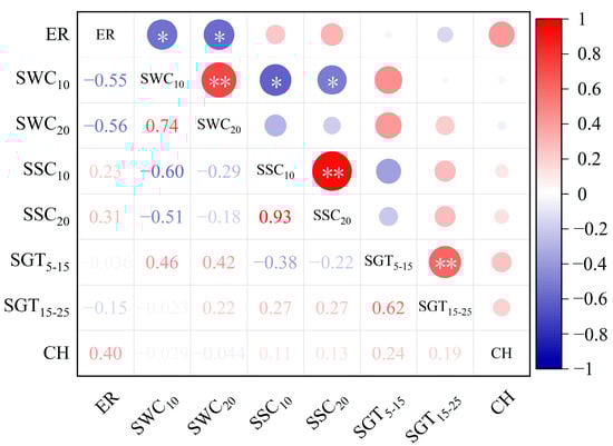
Figure 12.
Correlation analysis between seedling emergence rate, soil water, heat, and salt, and plant height. Note: “*” indicates p < 0.05, significant correlation, “**” indicates p < 0.01, significant correlation. ER (cotton seedling emergence rate), SWC10 (average water content of 10 cm soil layer), SWC20 (average water content of 20 cm soil layer), SSC10 (average salt of 10 cm soil layer), SSC20 (average salt of 20 cm soil layer), SGT5–15 (average soil temperature within 5–15 cm), SGT15–25 (average soil temperature within 15–25 cm), CH (plant height of cotton seedlings).
The average soil water content at 10 cm was highly significantly positively correlated with the average soil water content at 20 cm (p < 0.01), with a correlation coefficient of 0.74; the average soil water content at 10 cm was significantly negatively correlated with the average soil salt content at 10 cm (p < 0.05), with a correlation coefficient of −0.60; and the average soil water content at 10 cm was significantly negatively correlated with the average soil salt content at 20 cm (p < 0.05), with a correlation coefficient of −0.51.
The average soil salt content at 10 cm was highly significantly positively correlated (p < 0.01) with the average soil salt content at 20 cm, with a correlation coefficient of 0.93.
The average soil temperature from 5 to 15 cm was highly significantly positively correlated with the average soil temperature from 15 to 25 cm (p < 0.01), with a correlation coefficient of 0.62.
There was no significant correlation between the cotton seedling height, soil water, heat, and salt indexes, and seedling emergence rate.
3.2. HYDRUS-2D Model Calibration and Validation
3.2.1. Determination of Model Hydraulic Parameters
Regarding the determination of the soil hydraulic parameters in the Van Genuchten [24] model, the soil particle composition was obtained through a particle size analyzer, the initial hydraulic parameters were obtained according to the Rosetta Lite module that comes with HYDRUS-2D, and the hydraulic parameters after being determined by the soil water content rate are shown in Table 3. The related parameters such as longitudinal dispersion (DL) and transverse dispersion (DT) in solute transport were referred to the relevant HYDRUS-2D soil water–salt transport references [25], and the longitudinal dispersion DL after rate-setting through soil salinity was 30 cm. The transverse dispersion DT was 3 cm, the molecular diffusion coefficient (DW) in free water was 2.14 cm2/d, and the molecular diffusion coefficient (DG) in soil air was 0 cm2/d.
Table 3.
Soil hydraulic parameters.
3.2.2. Model Calibration and Validation
This article uses the measured values of the soil water content and soil salt content in the T2 treatment for model calibration and uses the measured values of the soil water content and soil salt content in the T1 and T3 treatments for model validation.
As shown in Table 4, the measured values and simulated values of the soil water content in the T2 treatment were calibrated, and the model evaluation indexes showed that R2 was greater than 0.85, the range of the RMSE values was between 1.89 and 2.37 cm3·cm−3, and the range of MAE values was between 1.71 and 1.99 cm3·cm−3; the measured and simulated values of the soil water content were validated in the T1 and T3 treatments. The model evaluation indexes showed that R2 was not less than 0.87, the RMSE values were less than 2.12 cm3·cm−3, and the MAE values were not greater than 1.95 cm3·cm−3.
Table 4.
Evaluation of soil water content modeling results.
As shown in Table 5, the measured and simulated values of the soil salt in the T2 treatment were calibrated, and the model evaluation indexes showed that R2 was not less than 0.79, the RMSE values ranged from 1.07 to 1.51 g/kg, and the MAE values ranged from 0.92 to 1.40 g/kg; the measured and simulated values of the soil salt content were validated in the T1 and T3 treatments. The model evaluation indexes showed that R2 was greater than 0.79, the RMSE values were less than 1.33 g/kg, and the MAE values were not greater than 1.23 g/kg.
Table 5.
Evaluation of soil salt content modeling results.
3.3. Simulation of Soil Water and Salt Transport Processes under Different Scenarios
3.3.1. Model Scenario Simulation Settings
The hydraulic parameters and solute transport parameters of the calibrated model were used to simulate the water and salt transport during the cotton seedling stage in the experimental area. The simulation period was from 16 April to 30 April 2024, and the simulation time was 15 days. The scenarios were set with different irrigation amounts and frequencies, and there were 20 scenarios in total, as shown in Table 6.
Table 6.
Scenarios simulation—irrigation regime for cotton seedling stage.
3.3.2. Simulation of Soil Water Transport Processes
The change processes of the soil water content under the different scenarios are shown in Figure 13. In all scenario simulations, the soil water content showed the trend of first increasing and then decreasing after irrigation and finally tended to stabilize, and the soil water content in the soil layer of 10–40 cm reached its peak value in the first day after the end of irrigation, with soil water content values of 10 cm > 40 cm > 30 cm > 20 cm.
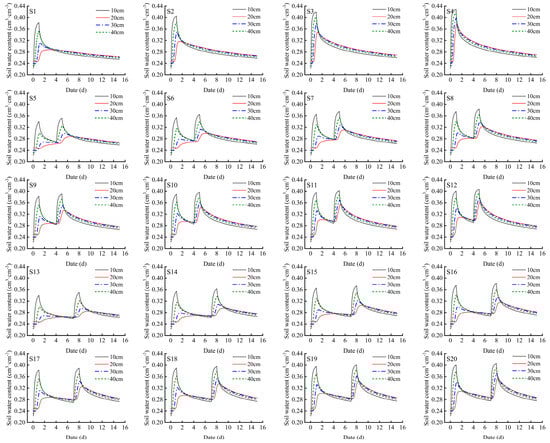
Figure 13.
Soil water changes under different scenarios. Note: the simulated soil water content in this figure is the soil water content of the 10–40 cm soil layer between the drip head and the cotton row.
For the treatment with a 14-day irrigation interval (S1–S4), as the irrigation amount increased, the soil water content of each soil layer also increased. At 15 days, the average soil water content of the S4 treatment was 0.007 cm3·cm−3 higher than that of the S1 treatment.
For the treatments with a 4-day irrigation interval (S5–S12), as the irrigation amount increased, the soil water content of each soil layer also increased. The peak value of the soil water content after the second irrigation was slightly higher than that after the first irrigation. Before the second irrigation, the soil water content in the 10–40 cm soil layer under the different treatments showed a trend of first increasing, then decreasing, and then increasing again. The trend of the soil water content in the 20 cm soil layer was not significant. At 15 days, the average soil water content of the S12 treatment was 0.011 cm3·cm−3 higher than that of the S5 treatment.
For the treatments with a 7-day irrigation interval (S13–S20), as the irrigation amount increased, the soil water content of each soil layer also increased. The peak value of the soil water content after the second irrigation was slightly higher than that after the first irrigation, and the change in the soil water content in the 20 cm soil layer was greater than the change in the soil water content treated with a 4-day irrigation interval. At 15 days, the average soil water content of the S20 treatment was 0.015 cm3·cm−3 higher than that of the S13 treatment.
For treatments with different irrigation intervals for the same irrigation amount, the average soil water content in the 10–40 cm soil layer was as follows: irrigation interval of 7 days > irrigation interval of 4 days > irrigation interval of 14 days.
3.3.3. Simulation of Soil Salt Transport Process
The change processes of the soil salt content under the different scenarios are shown in Figure 14. In all scenario simulations, the soil salt content showed the trend of first decreasing and then increasing after irrigation, and on the second day after irrigation the soil salt content in the 10–40 cm soil layer decreased significantly. The soil salt content was 20 cm > 30 cm > 40 cm > 10 cm, which was opposite to the ordering of the soil water content and also shows the basic knowledge that “salt follows water”.
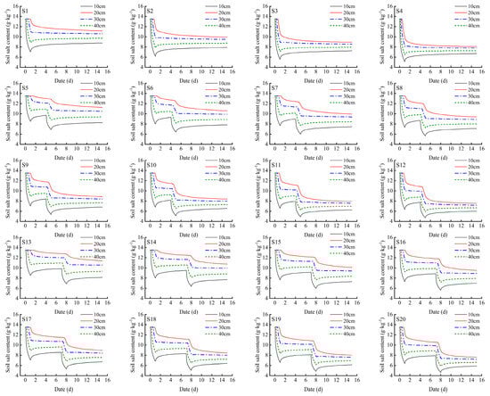
Figure 14.
Soil salt changes under different scenarios. Note: the simulated soil salt content in this figure is the soil salt content of the 10–40 cm soil layer between the drip head and the cotton row.
For the treatment with a 14-day irrigation interval (S1–S4), as the irrigation amount increased, the soil salt content of each soil layer gradually decreased. At 15 days, the average soil salt content of the S4 treatment was 2.588 g/kg lower than that of the S1 treatment.
For the treatment with a 4-day irrigation interval (S5–S12), as the irrigation amount increased, the soil salt content of each soil layer gradually decreased. The peak value of the soil salt content after the second irrigation was slightly lower than that after the first irrigation. Before the second irrigation, the soil salt content in the 10–40 cm soil layer under the different treatments showed a trend of first decreasing, then increasing, and then decreasing again; the trend of soil salt content in the 20 cm soil layer was not significant. At 15 days, the average soil salt content of the S12 treatment was 3.000 g/kg lower than that of the S5 treatment.
For the treatment with a 7-day irrigation interval (S13–S20), as the irrigation amount increased, the soil salt content of each soil layer gradually decreased. The peak value of the soil salt content after the second irrigation was slightly lower than that of the first irrigation, and the change in the soil salt content at the 20 cm soil layer was lower than the change in the soil salt content treated with a 4-day irrigation interval. At 15 days, the average soil salt content of the S20 treatment was 3.038 g/kg lower than that of the S13 treatment.
For the treatments with different irrigation intervals for the same irrigation amount, the average soil salt content in the 10–40 cm soil layer was as follows: irrigation interval of 14 days > irrigation interval of 7 days > irrigation interval of 4 days.
3.4. Optimization of Drip Irrigation Regime for Cotton with “Dry Sowing and Wet Emergence”
We established a mathematical regression equation between the cotton emergence rate measured in Section 3.1.4 and the soil water and salt data between the drip heads and the cotton row. We substituted the soil water and salt data from the different scenario simulations into this regression equation to obtain the cotton emergence rate for each treatment under the different scenario simulations, and we took the optimal seedling emergence rate as the evaluation index for the cotton “dry sowing and wet emergence” irrigation regime.
The regression equation of the cotton seedling emergence rate y1 and soil water content θ in the 10–20 cm soil layer is as follows:
y1 = −0.8815 × θ2 + 43.86 × θ − 470.26, R2 = 0.953
The regression equation of the cotton seedling emergence rate y2 and soil salt content S in the 10–20 cm soil layer is as follows:
y2 = −2.0279 × S2 + 42.368 × S − 150.48, R2 = 0.982
According to Equations (21) and (22), 95.3% of the variation in the cotton seedling emergence rate was due to the different soil water content in the 10–20 cm soil layer, indicating a high degree of fitting; the variation in the soil salt in the 10–20 cm soil layer was 98.2%, indicating a high degree of fitting. So, the two regression equations were able to reflect the relationships between the cotton seedling emergence rate and the soil water content and soil salt, respectively.
Using the analytic hierarchy process (AHP) to calculate the weight of the soil water content and soil salt content, the analysis results showed that the weights of the soil water content were 76.3%, the weights of soil salt content were 23.7%, and the CI = 0.0 < 0.1 (consistency index), which satisfied the consistency test.
The relationships between the comprehensive cotton emergence rate y and y1, y2 are as follows:
y = 0.763 × y1 + 0.237 × y2
According to Table 7, for the different irrigation frequency treatments, the cotton seedling emergence rate gradually decreased with the increase in the irrigation amount. Of the treatments, the S1 treatment with a 14-day irrigation interval had the highest seedling emergence rate of 70.85%; the S12 treatment with a 4-day irrigation interval had the lowest seedling emergence rate of 28.33%. For the same irrigation amount, the size of the cotton seedling emergence rate was as follows: irrigation interval of 14-day > irrigation interval of 7-day > irrigation interval of 4 days. In descending order, the four treatments which had a cotton seedling emergence rate of 67% or more were as follows: S1 > S13 > S2 > S14. Therefore, it is recommended to choose the irrigation regime of “dry sowing and wet emergence” for cotton with a 14-day irrigation interval or 7-day irrigation interval, which can obtain a higher emergence rate.
Table 7.
The emergence rate of the cotton under the different scenarios of “dry sowing and wet emergence”.
4. Discussion
4.1. The Effect of Soil Water, Heat, and Salt on Cotton Emergence Rate under Different Water Amounts
Compared to traditional winter and spring irrigation, the core of the “dry sowing and wet emergence” technology is to drip a small amount of irrigation water after cotton sowing. This practice ensures the cotton seedling rate on the basis of the effective alleviation of the situation of agricultural water tension in southern Xinjiang. At the same time, it avoids the phenomenon of soil compaction and land quality degradation caused by excessive irrigation water in traditional irrigation methods, which is beneficial for the growth and development of cotton. Therefore, the “dry sowing and wet emergence” technology ensures that cotton receives timely and appropriate water supply during the early stages of growth, preventing growth limitations caused by insufficient water. It is of great significance for promoting cotton growth in southern Xinjiang and improving water resource utilization efficiency.
This study showed that under the under-membrane drip irrigation pattern, the emergence rate of the cotton was negatively correlated with the soil water content in the 0–20 cm soil layer, indicating that the larger the irrigation quota during the cotton emergence stage, the lower the emergence rate of the cotton.
The cotton emergence rate of the T3 treatment was the lowest in this experiment, which may be due to the higher irrigation quota, as a higher the soil water content in the soil reduces the oxygen content in the soil. This may affect the respiration and metabolic cycle of cotton seeds, resulting in the slowing down of seed germination or even rotting and other phenomena [26].
The average soil water content at 10 cm was significantly negatively correlated with the average soil salt content at 10 cm and 20 cm; this is because, according to the transport law of “salt follows water” [27], the larger the irrigation quota, the better the effect of salt washing from the soil surface layer within the membrane and the lower the salt content of the surface layer of the soil inside the membrane. This is consistent with the research results of Zhang Wei et al. [28]. The soil salt in the bare land between the membranes was greater than that within the membranes, which was also because the soil water content in the bare soil between the membranes was lower than that in the soil inside the membranes. In addition to the influence of the soil water and soil salt, maintaining a suitable soil temperature was also one of the indispensable factors to ensure cotton seedling emergence [29].
The optimal temperature for cotton seed germination is 18–22 °C [16], and too low a temperature will lead to difficulties in cotton seedling emergence, increase the risk of seed erosion by pathogens, and affect the germination and later growth of cotton seeds. In addition, too high a soil water content will increase the degree of soil compaction, increase soil density, and reduce soil permeability, which is also unfavorable to the growth of the seed root system [30].
In this study, the emergence rates of the T1, T2, and T3 treatments did not reach 80%, which may be attributed to the following reasons: Firstly, the soil in the experimental area belongs to severely saline–alkali land, and the soil salt has an inhibitory effect on the cotton seedling emergence; although the salt tolerance of the Xinluzhong 55 variety is relatively strong, the soil salt in the cotton rows ranges position was between 7 and 14 g/kg, and the soil salt was still relatively high. Secondly, the amount of seedling emergence water was set to be too large, which resulted in the cotton rows having too much water near the cotton rows, affecting the respiration of the cotton seeds and subsequently affecting seed germination and emergence.
4.2. Simulation of Soil Water and Salt Distribution Patterns Based on the HYDRUS-2D Model
The results of the water–salt change rule simulated by the HYDRUS-2D scenario showed that, when the initial water content of the soil and the irrigation quota were certain, the average soil water content of the treatment with an irrigation frequency of twice was higher than that of the treatment with an irrigation frequency of once in the soil layer of 10–40 cm on the 15th day; the average soil water content of the treatment with an irrigation interval of 7 days was higher than that of the treatment with an irrigation interval of 4 days, which is because the irrigation frequency can change the spatial distribution of the soil water and soil water storage [31]. Under the condition of the same amount of irrigation, increasing the irrigation frequency can increase the water content of the upper soil layer, making the soil better maintain a moist state. Secondly, according to the study by Bai Xueer et al. [32], 24 h after the end of irrigation, the water content within the wetted body reached a relatively stable state. Therefore, compared to the treatment with a 4-day irrigation interval, the treatment with a 7-day irrigation interval can more effectively utilize the residual water in the soil during the two irrigation periods, which increases the average water content of the soil.
For the soil salt, the salt content in the soil decreased with the increase in the irrigation quota. On the 15th day, within the 10–40 cm soil layer, the average soil salt content of the treatment with two irrigation times was lower than that of the treatment with one irrigation time, and the average soil salt of the treatment with an irrigation interval of 14 days was higher than that of the treatments with irrigation intervals of 7 and 4 days. This was because, according to the research of Wu Xuan [33] and Liu Tao et al. [34], increasing the irrigation frequency can increase the water content of the upper soil layer, which is beneficial for salt washing. This indicates that, under certain conditions, increasing the irrigation frequency can effectively reduce the average salt content of the soil. After irrigation stops, the salt content in the soil gradually moves upward with the evaporation of soil water [35], accumulating in the surface layer of the soil and causing the phenomenon of salt return, resulting in higher salt contents in treatments with longer irrigation intervals.
4.3. Optimization and Effect Analysis of “Dry Sowing and Wet Emergence” Irrigation Regime for Cotton
In this study, the cotton seedling emergence rate of one film, three tubes, and three rows was quadratically related to the soil water content. The cotton emergence rate decreased with the increase in the soil water content, which was consistent with the research results of Hu Qiongjuan et al. [36]; the cotton seedling emergence rate was quadratically related to the soil salt content, which was consistent with the results of Xu Xin et al. [37] and was slightly different from the results of Wang Fei [38] and Zhong Zhibo [39], among others. The reason may be that there were differences in the seed quality of the supplied cotton varieties, and the adaptability to soil conditions was also different. Some varieties may have a stronger salt tolerance, which makes it possible to maintain a higher seedling emergence rate in soils with higher soil salt. Secondly, there are differences in the environments of the experimental areas: the above experimental areas are located in the northern Xinjiang region, while this study is located in the southern Xinjiang region, and climatic conditions such as temperature, precipitation, and light all affect the seedling emergence rate. For the cotton emergence rate under the different scenarios, the soil water content in the 0–20 cm soil layer played a dominant role, and there was a non-linear negative correlation between the cotton emergence rate and soil water content. This indicates that the larger the soil water content was, the lower the cotton emergence rate was. The average emergence rate in the treatment with a 14-day irrigation interval was higher than that in the treatment with a 7-day interval and higher than that in the treatment with a 4-day interval. This indicates that the longer the irrigation interval, the lower the soil water content in the 0–20 cm soil layer. The oxygen content in the soil may also be relatively high, which is favorable for seed respiration, thus resulting in a higher emergence rate.
The common planting patterns for the cotton included one film, three tubes, and six rows (the wide row, narrow row, and inter-film distances were 66 cm, 10 cm, and 46 cm, respectively, with drip irrigation tape laid in the middle of the narrow row, with a film width of 205 cm), 1 film, 2 tubes, and 4 rows (the wide row, narrow row, and interfilm distances were 40 cm, 20 cm, and 40 cm, respectively, with drip irrigation tape laid in the middle of the narrow row, with a film width of 125 cm). In order to more intuitively demonstrate the impact of “dry sowing and wet emergence” technology on the cotton emergence under the different planting patterns, we selected the higher emergence rates of the S2 (irrigation frequency one time, total irrigation amount 450 m3/hm2) and S13 (irrigation frequency two times, total irrigation amount 300 m3/hm2) scenarios for comparative analysis. The soil water and salt comparisons after irrigation in the different planting patterns are shown in Figure 15 and Figure 16.
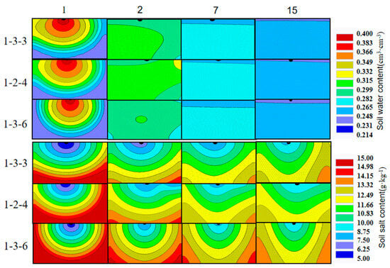
Figure 15.
Water and salt changes under different planting patterns in S2 scenario. Note: The numbers on the left side of the image represent the cotton planting mode. For example, 1-3-3 represents one film, three tubes, and three rows. The number at the top of the image represents the number of days after stopping watering. For example, 1 represents the first day after stopping watering. The first to third lines of the image show changes in soil water content, while the fourth to sixth lines show changes in soil salt content.
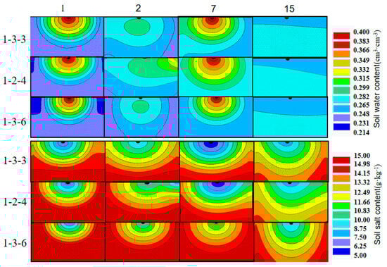
Figure 16.
Water and salt changes under different planting patterns in S13 scenario. Note: The numbers on the left side of the image represent the cotton planting mode. For example, 1-3-3 represents one film, three tubes, and three rows. The number at the top of the image represents the number of days after stopping watering. For example, 1 represents the first day after stopping watering. The first to third lines of the image show changes in soil water content, while the fourth to sixth lines show changes in soil salt content.
The variation patterns of the soil water and salt in Figure 15 and Figure 16 are consistent. On the first day after irrigation, the soil water content of the 10–40 cm soil layer in the one film, three tubes, and three rows showed no regularity with the depth of the soil layer, while the soil water content of the 10–40 cm soil layer in the one film, two tubes, and four rows and one film, three tubes, six rows decreased with the increase in the depth of the soil layer. On the 15th day, the soil water content of the 20 cm soil layer in the one film, three tubes, and three rows was the highest, and the soil water content of the 10 cm soil layer was the lowest. The soil water content of the 10–40 cm soil layer in the one film, two tubes, and four rows and one film, three tubes, six rows increased with the increase in the depth of the soil layer, while the soil salt change rule was just the opposite of the water. On the 15th day after irrigation, the soil water content of the 10–40 cm soil layer in the one film, three tubes, and three rows showed no regularity with the depth of the soil layer, while the soil salt content of the 10–40 cm soil layer in the one film, two tubes, and four rows and one film, three tubes, and six rows increased with the increase in the depth of the soil layer. The planting pattern with the lowest average soil salt content in the 10–40 cm soil layer was the one film, two tubes, and four rows planting pattern, while the planting pattern with the highest soil salt content was the one film, three tubes, and three rows planting pattern.
The emergence rates of the cotton under the different planting patterns in the S2 and S13 scenarios are shown in Table 8. In the S2 scenario, the emergence rate of one film, three tubes, and three rows was the highest, while the emergence rate of one film, two tubes, and four rows was the lowest. In the S13 scenario, the emergence rate of one film, three tubes, and three rows was the highest, while there was no significant difference between one film, two tubes, and four rows and one film, three tubes, and six rows. Therefore, overall, for severely saline–alkali land, one film, three tubes, and three rows may perform better in terms of the emergence rate.
Table 8.
Seedling emergence rate under different planting patterns.
Compared to the planting patterns of one film, two tubes, and four rows and one film, three tubes, and six rows, the one film, three tubes, and three rows planting pattern may require less water to achieve the same irrigation effect. Three drip irrigation belts can more accurately control water distribution and reduce water waste. However, due to the influence of various complex factors in the actual planting process, such as soil conditions, climate conditions, cultivation management, etc., the reasonable application of the dry sowing and wet emergence irrigation regime still needs to be analyzed and judged based on specific situations.
5. Conclusions
- (1)
- The average water content of the soil in the 0–40 cm soil layer within the membrane showed a trend of increasing and then decreasing over time, while the average water content of the soil in the 0–40 cm soil layer in the bare ground between the membranes showed a gradual increase over time; the average salt content of the soil in the 0–40 cm layer within the membrane and in the bare ground between the membranes showed a general trend of decreasing and then increasing over time.
- (2)
- The seedling vigor index of the T2 treatment was 25.9, and the highest cotton seedling emergence rate was 67.79%. The seedling vigor index of the T3 treatment was only 16.7, and the lowest cotton seedling emergence rate was 63.93%. Therefore, the appropriate reduction in irrigation amount can moderately improve the seedling emergence rate and seedling emergence index of cotton seeds.
- (3)
- In the 20 scenario simulations, under the same irrigation amount, the average soil water content in the 10–40 cm soil layer was as follows: irrigation interval of 7 days > irrigation interval of 4 days > irrigation interval of 14 days. The average soil salt content in the 10–40 cm soil layer was as follows: irrigation interval of 14 days > irrigation interval of 7 days > irrigation interval of 4 days.
- (4)
- By establishing the regression equations of the seedling emergence rate with the soil water content and soil salt content under the planting pattern of one film, three tubes, and three rows, it is recommended to choose the irrigation regime of “dry sowing and wet emergence” for cotton with medium–low water (300–450 m3/hm2) at 14-day intervals, or medium–low water (300–375 m3/hm2) at 7-day intervals, to achieve a higher seedling emergence rate.
Author Contributions
Conceptualization, H.W. and C.W.; methodology, H.W.; software, H.W.; validation, H.W.; investigation, H.W.; writing—original draft preparation, H.W.; writing—review and editing, C.W. All authors have read and agreed to the published version of the manuscript.
Funding
This research was funded by Corps Financial Science and Technology Plan Projects of Xinjiang Province, China (grant number 2022DB020) and the National Natural Science Foundation of China (grant number 52369012).
Data Availability Statement
The original contributions presented in the study are included in the article; further inquiries can be directed to the corresponding author.
Acknowledgments
Thanks to the editor and anonymous reviewers who significantly helped improve this manuscript; thank you to Yuefa Yang, Da Qin, Zikang Fan, Bo Li, and Xiaoyu Li from the research group for their assistance during the experiment.
Conflicts of Interest
The authors declare no conflicts of interest.
References
- Jans, Y.; von Bloh, W.; Schaphoff, S.; Müller, C. Global cotton production under climate change-Implications for yield and water consumption. Hydrol. Earth Syst. Sci. 2021, 25, 2027–2044. [Google Scholar] [CrossRef]
- Meng, Z.; Ran, Y.Q. Current issues and countermeasures for the high-quality development of Xinjiang’s cotton industry. South China Agric. 2023, 17, 240–243+247. [Google Scholar] [CrossRef]
- Wang, Y.Q.; Zhang, W.T.; Tian, C.Y.; Mai, W.X. Application, Problems and Solution Strategies of “Dry Sowing and Wet Emergence” Planting Technology of Cotton in Southern Xinjian. Chin. Agric. Sci. Bull. 2024, 40, 62–65. [Google Scholar]
- Xiao, C.; Li, M.; Fan, J.L.; Zhang, F.C.; Li, Y.; Cheng, H.L.; Li, Y.P.; Hou, X.H.; Chen, J.Q. Salt leaching with brackish water during growing season improves cotton growth and productivity, water use efficiency and soil sustainability in southern Xinjiang. Water 2021, 13, 2602. [Google Scholar] [CrossRef]
- Chen, X.L.; Sun, C.M.; Liu, P. The practice of cotton “sowing drily and emerging wet” technology in Korla, Xinjiang. China Cotton 2021, 48, 41–42+45. [Google Scholar]
- Wang, J.S.; Wang, Y. Effect of Dry Seeding and Wet Budding of Cotton with Drip Irrigation under plastic film. J. Tarim Univ. 2006, 1, 77–78. [Google Scholar] [CrossRef]
- Chen, S.S.; Pei, D.; Wang, Z.H.; Zhang, X.Y.; Chen, S.Y.; Sun, H.Y. Influence of irrigation modes on water consumption and yield of cotton with drip irrigation under plastic mulch in North China Plain. Agric. Res. Arid Areas 2005, 6, 30–35. [Google Scholar] [CrossRef]
- Li, L.; Dong, H.L.; Ma, Y.Z.; Li, P.C.; Li, C.M.; Zhang, N.; Wan, S.M.; Xu, W.X. Effects of Row Spacing Patterns on the Growth, Yield and Quality of Machine-picked Cotton. Xinjiang Agric. Sci. 2020, 57, 713–721. [Google Scholar]
- Zheng, M.; Bai, Y.G.; Zhang, J.H.; Liu, H.B.; Wang, B.; Xiao, J.; Ding, Y.; Han, Z.Y. Effects of irrigation quantity and irrigation frequency of dry sowing and wet seedling on soil compaction, water salt distribution and seedling emergence in cotton fields. Agric. Res. Arid Areas 2022, 40, 100–107. [Google Scholar] [CrossRef]
- Shao, J.J.; Li, P.C.; Zheng, C.S.; Sun, M.; Feng, W.N.; Zhang, X.L.; Dong, H.L. Effects of salt stress on emergence rate and development of cotton seedlings under dry-sowing and wet-emergence planting mode. Cotton Sci. 2023, 35, 288–301. [Google Scholar] [CrossRef]
- Dong, X.; Chai, Z.P.; Bai, Y.G.; Liu, H.B.; Ding, Y.; Xiao, J. Effect of Different “Dry Broadcast and Wet Surface” Planting Method on Soil Water, Heat, Salt and Yield in Cotton Fields in Southern Xinjiang. Water Sav. Irrig. 2024, 2, 33–40. [Google Scholar] [CrossRef]
- Ding, Y.; Zhang, J.H.; Bai, Y.G.; Zhao, J.H.; Zheng, M.; Liu, H.B.; Xiao, J.; Han, Z.Y. Study on the effects of different water treatments on the emergence rate of cotton. Xinjiang Agric. Sci. 2023, 60, 2380–2389. [Google Scholar] [CrossRef]
- Zhang, M.Z.; Li, Q.H.; Shi, X.L. Soil Science and Agronomy; China Water & Power Press: Beijing, China, 2007. [Google Scholar]
- Du, M.Q.; Wu, R.J.; Yang, M.F. Comparative Study of Drying Weighing Method and TDR Method for Observing Soil Moisture. Technol. Soil Water Conserv. 2018, 4, 7–9. [Google Scholar] [CrossRef]
- Chen, W.; Li, M.; Li, Q. The Influence of Winter Irrigation Amount on the Characteristics of Water and Salt Distribution and WUE in Different Saline-Alkali Farmlands in Northwest China. Sustainability 2023, 15, 15428. [Google Scholar] [CrossRef]
- Xu, H.X.; Yang, W.H.; Wang, Y.Q.; Zhou, D.Y.; Xia, J.Y.; Feng, X.A. Effect of temperature on seed vigor of cotton. China Cotton 2004, 2, 15–16. [Google Scholar] [CrossRef]
- Yi, G.; Quan, J.W.; Kang, W. Spring irrigation with magnetized water affects soil water-salt distribution, emergence, growth, and photosynthetic characteristics of cotton seedlings in Southern Xinjiang, China. BMC Plant Biol. 2023, 23, 174. [Google Scholar] [CrossRef]
- Nasr, H.M.; Selles, F. Seedling emergence as influenced by aggregate size, bulk density, and penetration resistance of the seedbed. Soil Till. Res. 1995, 34, 61–76. [Google Scholar] [CrossRef]
- Simunek, J.; Sejna, M.; van, G. The Hydrus-2D Software Package for Simulating Two-Dimensional Movement of Water, Heat, and Multiple Solutes in Variably Saturated Media; Version 2.0, IGWMC-TPS-53; International Ground Water Modeling Center, Colorado School of Mines: Golden, CA, USA, 1999; p. 251. [Google Scholar]
- Li, Z.R.; Hu, D.; You, G.D. Experiment and simulation on salt removing of drip irrigation under the film in cotton field. J. Shihezi Univ. 2018, 36, 376–384. [Google Scholar] [CrossRef]
- Wang, S.X.; Dong, X.G.; Wu, B.; Yang, P.N. Numerical simulation and control mode of soil water and salt movement in arid salinization region. Trans. Chin. Soc. Agric. Eng. 2012, 28, 142–148. [Google Scholar] [CrossRef]
- Wu, M.H.; Wang, Y. Characteristics and influencing factors of crop water demand and yield in Shache irrigation area of Xin-jiang. Chin. J. Ecol. 2023, 42, 1858–1868. [Google Scholar] [CrossRef]
- Simunek, J.; Sejna, M.; van Genuchten, T. HYDRUS-2D. 1999. Available online: https://www.pc-progress.com/en/Default.aspx?hydrus-2d (accessed on 5 September 2024).
- Van Genuchten, M.T. Closed-form Equation for Predicting the Hydraulic Conductivity of Unsaturated Soils. Soil Sci. Soc. Am. J. 1980, 44, 892–898. [Google Scholar] [CrossRef]
- Phogat, V.; Pitt, T.; Stevens, R.M.; Cox, J.W.; Šimůnek, J.; Petrie, P.R. Assessing the role of rainfall redirection techniques for arresting the land degradation under drip irrigated grapevines. J. Hydrol. 2020, 587, 125000. [Google Scholar] [CrossRef]
- Xu, M.; Li, J.L.; Ye, F.M.; Zhu, H.; Wang, Z.S. Effects of Temperature and Humidity on Cotton Seed Germination. J. Agric. 2022, 12, 10. [Google Scholar]
- Du, X.J.; Yan, B.W.; Xu, K.; Wang, S.Y.; Gao, Z.D.; Ren, X.Q.; Hu, S.W.; Yun, W.J. Research Progress on Water-salt Transport Theories and Models in Saline-alkali Soil. Chin. J. Soil Sci. 2021, 52, 713–721. [Google Scholar] [CrossRef]
- Zhang, W.; Lv, X.; Li, L.H.; Liu, J.G.; Sun, Z.J.; Zhang, X.W.; Yang, Z.P. Salt transfer law for cotton field with drip irrigation under the plastic mulch in Xinjiang Region. Trans. CSAE 2008, 24, 15–19. [Google Scholar]
- Zhang, X.M.; Guo, K.; Xie, Z.X.; Fen, X.H.; Liu, X.J. Effect of frozen saline water irrigation in winter on soil salt and water dynamics, germination and yield of cotton in coastal soils. Chin. J. Eco-Agric. 2012, 20, 1310–1314. [Google Scholar] [CrossRef]
- Yu, Q.; Zhang, H.L.; Chai, Q.; Li, Z.J.; Tang, S.J. Effects of different soil moistures on emergence and root of Kentucky bluegrass. Pratacultural Sci. 2013, 30, 1338–1343. [Google Scholar]
- Cao, H.X.; Kang, S.Z.; He, H. Effects of evaporation and irrigation frequency on soil water distribution. Trans. Chin. Soc. Agric. Eng. 2003, 6, 1–4. [Google Scholar] [CrossRef]
- Bai, X.E.; Ai, Y.D.; Yang, H.S.; Ge, Y.X.; Xing, Z.; Hu, X.T.; Zhou, S.W. Effects of Different Initial Water Content and Dripper Discharge on Wetted Body Characteristic of Drip Irrigation. J. Irrig. Drain. 2019, 38, 73–78. [Google Scholar] [CrossRef]
- Wu, X. Characteristics of Salt and Water Movement and Numerical Simulation in Greenhouse Soil under Different Irrigation Frequencies. Sichuan Agricultural University. 2014. Available online: https://kns.cnki.net/kcms2/article/abstract?v=QenloEQs_R8N3SMS8ribVPkoDzm2RACZNQnYjmuvZemPk8Is55XboPbrNiJOwXQSPJCmVuBsZ-CXmmTrkxIEg4Yc41qP55fygRghzB8JxlHjQHlMcgn78u7UsfHnDdEpVNkfs8r7mEJknpiwTlTao7X085fhSNo34cr0cRtNkVM198Kft7IGD4ZXcufRgwQ1IHqgXfIxmCU=&uniplatform=NZKPT&language=CHS (accessed on 5 September 2024).
- Liu, T.; Wu, X.; Zheng, Z.C.; Li, Y.X. Effects of Irrigation Frequency on Water and Salt Movement in Greenhouse Soil. J. Ecol. Rural Environ. 2016, 32, 622–631. [Google Scholar] [CrossRef]
- Tan, J.L.; Wang, X.N.; Tian, J.C.; Su, X.L. Effect of gravel-sand mulching on movements of soil water and salts under different amounts of brackish water. Trans. Chin. Soc. Agric. Eng. 2018, 34, 100–108. [Google Scholar] [CrossRef]
- Hu, Q.J.; Zheng, M. Study on the Convelation Between Soil Environment of “Dry Sowing and Wet Germination” and Cotton Emergence Rate in Southern Xinjiang. Heilongjiang Agric. Sci. 2023, 10, 6–12. [Google Scholar] [CrossRef]
- Xu, X.; Zhang, J.Z.; Li, B.Z.; Wang, Z.H.; Li, W.H. Response characteristics and numerical simulation of soil water and salt dynamics in different salinized cotton seedling stage to submembrane drip irrigation. J. Shihezi Univ. 2022, 40, 204–212. [Google Scholar] [CrossRef]
- Wang, F.; Lv, D.S.; Wang, Z.H.; Zhang, J.Z.; Liu, J.; Wen, Y.; Qin, C.; Hu, G.R. Effects of water-salt coupling on seeding emergence rate and seeding growth of cotton under drip irrigation. Water Sav. Irrig. 2023, 3, 91–97. [Google Scholar] [CrossRef]
- Zhong, Z.B.; He, S.; Zhang, W.H.; Zhou, J.W.; Zhen, G.Y.; Ma, J.Y.; Cheng, H.; Shi, C.; Zhang, X. Study on cotton formation and water salt transportation under salinization. Xinjiang Agric. Sci. 2023, 60, 2390–2395. [Google Scholar] [CrossRef]
Disclaimer/Publisher’s Note: The statements, opinions and data contained in all publications are solely those of the individual author(s) and contributor(s) and not of MDPI and/or the editor(s). MDPI and/or the editor(s) disclaim responsibility for any injury to people or property resulting from any ideas, methods, instructions or products referred to in the content. |
© 2024 by the authors. Licensee MDPI, Basel, Switzerland. This article is an open access article distributed under the terms and conditions of the Creative Commons Attribution (CC BY) license (https://creativecommons.org/licenses/by/4.0/).