Abstract
Causal discovery is a highly promising tool with a broad perspective in the field of biology. In this study, a causal structure robustness assessment algorithm is proposed and employed on the causal structures obtained, based on transcriptomic, proteomic, and the combined datasets, emerging from a quantitative proteogenomic atlas of 15 sweet cherry (Prunus avium L.) cv. ‘Tragana Edessis’ tissues. The algorithm assesses the impact of intervening in the datasets of the causal structures, using various criteria. The results showed that specific tissues exhibited an intense impact on the causal structures that were considered. In addition, the proteogenomic case demonstrated that biologically related tissues that referred to the same organ induced a similar impact on the causal structures considered, as was biologically expected. However, this result was subtler in both the transcriptomic and the proteomic cases. Furthermore, the causal structures based on a single omic analysis were found to be impacted to a larger extent, compared to the proteogenomic case, probably due to the distinctive biological features related to the proteome or the transcriptome. This study showcases the significance and perspective of assessing the causal structure robustness based on omic databases, in conjunction with causal discovery, and reveals advantages when employing a multiomics (proteogenomic) analysis compared to a single-omic (transcriptomic, proteomic) analysis.
1. Introduction
The elucidation of gene and protein expression, along with their interplays, stands as a cornerstone in biological sciences [1]. Transcriptome profiling on a large scale has gained traction as a primary technique to scrutinize the variety within biological specimens. Such analyses have traditionally been organ-specific or encompass entire entities, like plants, but there is a growing emphasis on detailed transcriptome profiles of distinct tissues or cells due to their potential to unravel gene functionality [2].
The field of proteogenomics emerged as an innovative approach, expanding the scope of genomic analysis through the integration of transcriptomic and proteomic data [3]. This methodological fusion seeks to concurrently examine alterations at the genetic level—such as mutations, polymorphisms, and insertions/deletions—with those at the protein level [4]. Proteogenomic databases are pivotal in correlating gene expression with protein production, thereby enhancing the comprehension of gene models [3,5,6]. Beyond its established utility in augmenting genome annotation and protein identification in non-model plant species [7], proteogenomics holds considerable promise in biotechnological endeavors, particularly plant breeding. For instance, proteogenomics facilitates a detailed elucidation of biosynthetic pathways, aiming to augment agronomic traits, a concept recently applied to pear breeding through gene co-expression module analysis [8]. Furthermore, proteogenomic analyses contribute to the exploration of alternative splicing events and post-translational modifications in plant species [9]. An application of proteogenomic analysis has also been noted in examining the role of carbamoyltransferase genes during the ripening of fleshy fruits [10]. Nonetheless, the development of bioinformatic tools to adeptly manage and interpret this wealth of proteogenomic data for actionable insights remains in its nascent stages [6].
Causal models are used to investigate the structure of causal relationships between different variables. Causal discovery justifies the causal nature of a relationship between two variables based on its persistence [11]. An advantage of causal model development, compared to traditional statistical association, is the existence of direction in the causal relationships between variables, which characterizes the cause and the effect variable in each relation [11]. This is of particular importance in several scientific fields, including biology, and contrasts with the typically used correlation indices, which are mostly bidirectional. Thus, causal discovery demonstrates a wide potential in the field of biology. Obtaining the causal structure may validate expectations and/or uncover new knowledge, facilitating scientific interpretations. Causal discovery has been used in the literature within different contexts (see, e.g., [12,13,14,15,16,17]). Particularly, in the field of genetics, causal methods or their underlying ideas have been applied, among else, to detect causal relationships among phenotypes [18,19] to infer gene regulatory networks [20,21,22,23,24,25], and to infer causal associations between gene expression and disease [26]. A more detailed discussion on causal discovery in biology can be found in Glymour et al. [27].
Causal structure investigation and Directed Acyclic Graphs (DAGs), in particular, have been employed by our group in several studies that involved multiomics data. Employing causal structure learning in olive leaves and roots at a proteogenomic level, unveiled key interaction networks involved in salt priming in olive trees [28]. A causal model-based multiomics pipeline was introduced in Boutsika, et al. [29] to determine the molecular portrait of the PGI potatoes of the Naxos Island. Genome-wide DNA methylation, RNA sequencing and quantitative proteomics were exploited, revealing key environment-derived molecular factors, putative epimarkers and key microbes, relevant to authenticating Naxos potato [29]. In addition, causal discovery was employed in sweet cherry multiomics data, leading to understanding the cause–effect relationships that are important in the fruit softening and ripening process in sweet cherry (Prunus avium L.) [30]. The analysis in Ganopoulou et al. [30] was based on a plant tissue proteogenomic atlas that contains a combination of sweet cherry (Prunus avium L.) tree transcriptomic and proteomic datasets (represented by 29,247 genes and 7584 proteins, respectively), involving 15 sweet cherry tissue samples [31]. The sweet cherry, a perennial fruit tree belonging to the Rosaceae family, holds a prominent economic position globally [32,33,34]. Its non-climacteric ripening pattern distinguishes it from other Prunus species like peach and apricot, adding to the significance of its study [35].
A question arising when determining the causal structure is related to the robustness of the causal structure itself. Towards this direction, a causal structure robustness assessment approach has been recently introduced, aiming to assess the robustness of the causal relationships of genetic risk factors that affect the Syntax Score, an index that evaluates the complexity of coronary artery disease [36]. This approach investigated the impact on the obtained causal structures, both local and global, under different levels of interventions, reflected in the increasing number of patients (observations) that were randomly excluded from the datasets considered.
The aim herein was to propose a new causal structure robustness assessment algorithm, specifically designed for single-omic or multiomics data involving plant tissue samples, and employ sweet cherry as an example to apply it and assess the robustness of the related obtained causal structures. In contrast to Ganopoulou et al. [30], where causal discovery referred to the gene/protein consensus modules (clusters) that were obtained by employing weighted gene co-expression network analysis (WGCNA) [37], herein, it referred directly to the gene/proteins. The transcriptomic and proteomic data were separately considered at first, and the results were compared with the case when they were jointly used in a multiomics analysis. The proposed approach assesses the robustness of the obtained causal structures by evaluating the impact of intervening in the datasets of these causal structures using diverse criteria. The differences compared to the approach proposed in Ganopoulou et al. [36] are that, herein, each of the observations (plant tissues) involved is removed, one at a time, from the datasets (compared to the random exclusion of an increasing number of observations/patients in [36]), and the causal structure is re-determined and compared not only to the initial causal structure but, in addition, to the remaining re-determined causal structures. The reason for separately treating each tissue is that plant tissue samples are, in general, straightforwardly related to specific biological functions. Assessing the robustness of causal structures that are obtained, either in a single-omic or in a multiomics context, on top of validating causal discovery and related inferred knowledge and conclusions, may provide valuable insight regarding specific tissues and their impact when determining causal relationships.
2. Materials and Methods
2.1. Directed Acyclic Graphs (DAGs)
Bayesian networks constitute a distinct category of graphical models used for illustrating and explicating the causal relationships among random variables. These networks are constructed as DAGs that were initially proposed by Pearl [38]. DAGs employ nodes (or vertices) and directed edges (or arcs) as fundamental components to visualize the causal structure. Each node typically corresponds to a random variable. The graphical representation enables the visualization of statistical dependencies existing among various variables. Within the framework of DAGs, paths (or chains) are delineated as sequences of interconnected edges. If a directed edge connects variable to , is identified as the parent (or cause) of , while is considered the child (or effect) of . DAGs exhibit an acyclic structure, namely no paths of edges originating from a node and terminating at the same node exist.
A completed partially-directed acyclic graph (CPDAG) represents the Markov equivalence class of a DAG [39]. All DAGs that belong to a specific equivalence class describe the same conditional independence relationships since they are structured with the same skeleton (adjacencies) and the same v-structures. Assume is a DAG. The skeleton of is the undirected graph that is formed by removing the directions of all the edges in the DAG. A v-structure in is an ordered triplet of nodes (), such that contains the directions of and y←z; additionally, the nodes are not connected with an edge in . Some edges may exhibit an undetermined direction (so-called bidirected/undirected edges). This means that they have the opposite direction from one DAG in the equivalence class to another DAG in the same equivalence class.
2.2. Data Description
Sweet cherry cv. ‘Tragana Edessis’ tissue samples (15 in total) were collected (represented by 29,247 genes and 7584 proteins) related to the most important organs. In particular, the tissues covered the annual sweet cherry shoot (“1st Year shoot”), early growth leaves (“Young leaves”), fully developed leaves (“Leaves”), dormant flower (“Flower buds”), dormant vegetative buds (“Dormancy buds”, early in spring, ecodormancy stage), flowers at both white tip stage (“1st Bloom”) and full flowering phase (“Flower”). Sweet cherry fruit (exo-mesocarp) were sampled during four developmental stages, corresponding to the fruit set (8 days after full bloom [DAFB]; “Fruit 1st stage”), the beginning of fruit coloring from green to yellow (20 DAFB; “Fruit 2nd stage”), the coloring from yellow to red (34 DAFB; “Fruit 3rd stage”), and to the fruit ripe for harvest (44 DAFB; “Fruit 4th stage”). The corresponding stems were collected at the same developmental stages (“Stem 1st stage”, “Stem 2nd stage”, “Stem 3rd stage” and “Stem 4th stage”). More details can be found in Xanthopoulou et al. [31]. The transcript expression and protein abundances are available in the SweetBiOmics database (www.GrCherrydb.com, accessed on 1 September 2023).
2.3. Robustness Assessment Algorithm
The causal structure robustness assessment algorithm was tailored for single-omic or multiomics data involving plant tissue samples. It is focused on assessing the robustness of the related obtained causal structures by evaluating the impact of intervening in the datasets based on which these causal structures were determined. It entails the following steps:
- i.
- Determine/estimate the initial causal structure (CPDAG) based on the related omic database (assume that it entails plant tissues), using a selected causal structure learning algorithm.
- ii.
- Each of the plant tissues (observations) involved is removed, one at a time, from the database and the causal structure is re-determined, resulting in new causal structures (CPDAGs), each corresponding to a particular plant tissue excluded.
- iii.
- Each of the CPDAGs is compared to all CPDAGs (, both the initial and the re-determined CPDAGs), each of which is assumed to be the reference causal structure in each comparison.
- iv.
- The comparison is performed based on various metrics. In particular:
- a.
- The structural Hamming distance (SHD) between two CPDAGs [40]. This distance accounts for the number of operators required to make two CPDAGs match, or more specifically, to add or delete an undirected edge, and add, remove, or reverse the orientation of an edge. The SHD is computed for all pairs of CPDAGs.
- b.
- The percentage of common bidirected edges. The percentage of bidirected edges in each reference CPDAG that remained bidirected in each CPDAG.
- c.
- The percentage of common directed edges. The percentage of directed edges in each reference CPDAG that remained directed with the same direction in each CPDAG.
- d.
- The percentage of directed to bidirected edges. The percentage of directed edges in each reference CPDAG that turned into bidirected in each CPDAG.
- e.
- The percentage of directed edges that changed direction. The percentage of directed edges in each reference CPDAG that changed direction in each CPDAG.
- v.
- Hierarchical clustering is performed based on the above metrics and/or combinations of the metrics and is used to cluster the CPDAGs based on their comparison to all CPDAGs (when considered as the reference causal structures). In particular, the vectors, which correspond to the values of a selected metric when each of the CPDAGs is compared to all CPDAGs (reference causal structures), are used to hierarchically cluster the CPDAGs.
Reasoning
The reasoning within Steps (ii) and (iii) is that, since plant tissue samples are, in general, related to specific biological functions, by removing the data related to a specific plant tissue from the database and re-determining the causal structure, valuable insight may emerge pertained to this tissue. For example, based on the differences between the re-determined causal structure compared to the initial causal structure, conclusions can be drawn regarding the impact of a specific tissue on the estimated initial causal relationships. In addition, CPDAGs corresponding to the exclusion of biologically similar tissues (e.g., covering the same organ) may be expected to be similar. If not, it may be of interest to understand the differences in the corresponding causal structures. Moreover, two re-determined CPDAGs may exhibit many differences compared to the initial CPDAG, and at the same time be very similar to each other, or exhibit many differences as well when being compared to each other. The selection of criteria in step (iv) aimed to efficiently describe the CPDAGs comparison, based both on an overall assessment (SHD) and specific characteristics of the CPDAGs, such as similarities in bidirected/directed edges and changes that have occurred from one CPDAG to another. The reasoning within Step (v) is to evaluate the obtained CPDAG clusters and draw specific conclusions. An interesting aspect is to investigate whether CPDAGs corresponding to the exclusion of biologically similar tissues are clustered together.
2.4. Sweet Cherry Proteogenomic Atlas–Causal Structure Robustness Assessment
The analysis was based on the protein abundances and the transcript FPKMs in the Sweet Cherry Proteogenomic Atlas [31]. Initially, the pre-processing of the data was performed as described in Xanthopoulou et al. [31]. Additionally, only gene/protein pairs with valid values for all tissues at both proteomic and transcriptomic levels were selected (n = 7244). Of these, only the gene/protein pairs with values greater than 1 in at least 5 tissues (one out of three) at both protein and transcriptomic levels were further assessed, resulting in 6332 cases. Both the proteomic and the transcriptomic data were standardized per protein/gene ID across all 15 tissues.
Then, the causal structure robustness assessment algorithm, described in Section 2.3, was separately performed in three cases, (a) single-omic: only the transcriptomic data were considered (n = 6332, 15 tissues), (b) single-omic: only the proteomic data were considered (n = 6332, 15 tissues), and (c) multiomics: both the transcriptomic and the proteomic data were considered (n = 6332, 30 tissues).
At step (i) of the algorithm, the causal relationships among (a) the 6332 genes, (b) the 6332 proteins, and (c) the 6332 gene/protein pairs were initially determined based on all 15 tissues with the constrained-based PC algorithm [41,42], which is a common algorithm used to learn the structure of a causal Bayesian network, named after its inventors, Peter Spirtes and Clark Glymour. The CPDAG that was obtained was represented by “All15T” (in all three cases (a), (b) and (c)). It was typically assumed that causal sufficiency holds [11]. This condition implies that for each pair of measured variables, all their common direct causes are measured as well. That is to say, there are no hidden, unmeasured confounders for any pair of variables. The PC algorithm was applied using the R package “MXM” [43]. The skeleton of the causal network was developed with the function “pc.con”, which performs a faster implementation of the PC algorithm compared to the “pc.skel” function (in the same R package), but is limited to continuous data only as was the case in this study. The method argument was opted to be “pearson”, and the significance level “alpha” was set to 0.01, both being the default values in this function.
Then (step (ii)), each of the available 15 tissues was removed from each dataset, one at a time, and the causal structure was re-determined resulting in 15 newly determined CPDAGs in each case, based on 14, 14 and 28 tissues considered, respectively, ((a), (b) and (c)), since in the case of the proteogenomic analysis each tissue was removed from both datasets. These 15 re-determined CPDAGs were represented by “T”, where i = 1, 2, …, 15, corresponded to the ith tissue that was removed from the analysis. Namely, “T” stands for the CPDAG that was based on all 15 tissues except for the ith tissue. For example, if the 5th tissue was removed from a dataset, then the re-determined CPDAG was represented by “T5”. The order of the 15 tissues was “1st Bloom”, “1st Year shoot”, “Fruit 1st stage”, “Fruit 2nd stage”, “Fruit 3rd stage”, “Fruit 4th stage”, “Stem 1st stage”, “Stem 2nd stage”, “Stem 3rd stage”, “Stem 4th stage”, “Dormancy buds”, “Flower”, “Flower buds”, “Leaves”, and “Young leaves”. Thus, the corresponding CPDAGs when each of these 15 tissues was removed from each dataset were “T1”, “T2”, “T3”, …, “T14” and “T15”. The names of the CPDAGs were the same in all three analyses, i.e., “T3” represented the CPDAG not including the third tissue in the case of the transcriptomic, the proteomic analysis, and the proteogenomic analysis.
Next, each of the 16 CPDAGs (“All15T”, “T1”, “T2”, …, “T15”) was compared to all 16 CPDAGs in each case (step (iii)). In step (iv), the metrics employed were, the SHD, the percentage of the directed edges in each of the 16 causal structures (when considered as reference) that remained directed with the same direction in each of the 16 CPDAGs, and the percentage of the directed edges in each of the 16 reference CPDAGs that either remained directed with the same direction, or were transformed into a bidirected edge in each of the 16 CPDAGs. The above metrics were employed in hierarchical clustering in step (v). The hierarchical clustering was performed and visualized with the “pheatmap” function in R using the Euclidean as clustering distance and the complete clustering method. The absolute numbers of all the metrics in step (iv) of the algorithm ((iv) a–e, Section 2.3) were computed as well.
All the analyses were performed with the R programming language, Version 4.2.1.
3. Results
In the transcriptomic case, the results of the comparison based on the SHD and the percentage of the directed edges in each of the reference causal structures that remained directed with the same direction in each of the remaining causal structures are displayed in Figure 1. It is shown in Figure 1A that in the case that the 11th tissue (“Dormancy buds”) was removed from the transcriptomic database, the impact was the highest of all cases, since the CPDAG T11 exhibited the highest SHD compared to ALL15T (2256) among all CPDAGs, and, in addition, T11 exhibited the highest SHD to each of the reference CPDAGs, compared to all other CPDAGs. The smallest SHD compared to ALL15T was observed in the case of CPDAG T5 (882). Other than that, it was observed that CPDAGs corresponding to the removal of tissues with similar biological functions, such as tissues 3–6 (“Fruit 1st stage”, “Fruit 2nd stage”, “Fruit 3rd stage”, and “Fruit 4th stage”) were not clustered together in the heatmap. Similarly, the CPDAGs T7–T10 (“Stem 1st stage”, “Stem 2nd stage”, “ Stem 3rd stage”, and “ Stem 4th stage”), the CPDAGs T1–T13 (“Dormancy buds”, “Flower”, “Flower buds”), and T14–T15 (“Leaves”, “Young leaves”) were not clustered together as well (Figure 1A).
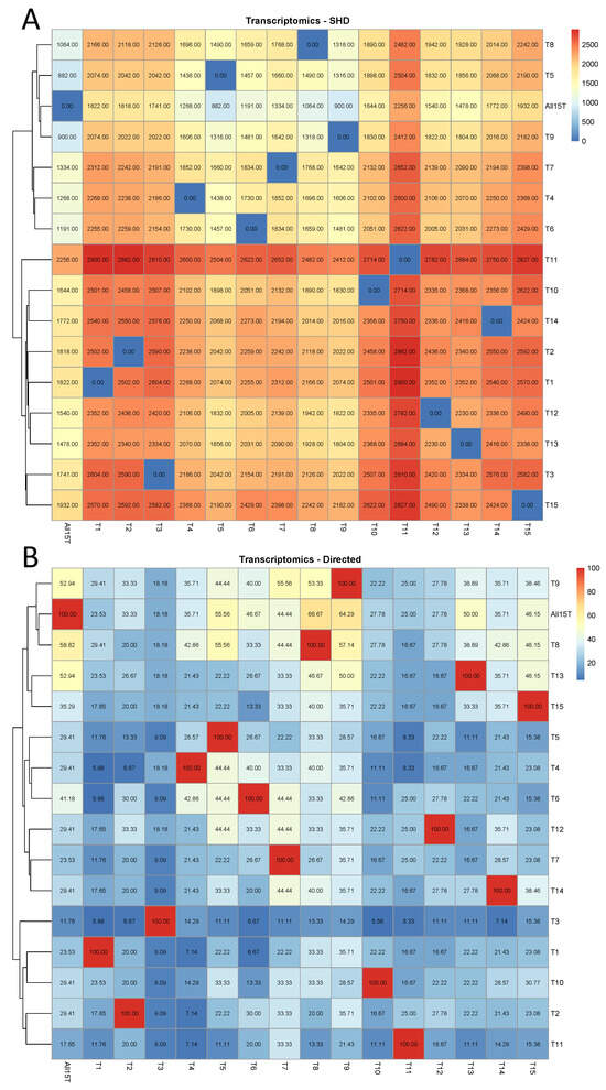
Figure 1.
Transcriptomic analysis. The comparison of each of the 16 CPDAGs (rows) to all 16 reference CPDAGs (columns) is displayed. Hierarchical clustering was performed by row. (A) SHDs, (B) The percentages of the directed edges in each of the reference causal structures that remained directed with the same direction in each of the 16 CPDAGs.
In the case of the assessment of the percentage of directed edges in each of the reference causal structures that remained directed with the same direction in each of the remaining 15 CPDAGs (Figure 1B), it was similarly observed that CPDAGs corresponding to the removal of tissues with similar biological function did not cluster together with the exception of CPDAGs T4–T6. In addition, CPDAG T3 (corresponding to the exclusion of “Fruit 1st stage”) was the one that exhibited the lowest percentage in almost all cases (except when compared to T4). The highest percentage (similarity in terms of directed edges) compared to ALL15T was observed in the case of CPDAG T8 (58.82).
Finally, when assessing the percentage of directed edges in each of the reference CPDAGs that either remained directed with the same direction or turned into bidirected, in each of the remaining causal structures (Figure A1), it was observed that the CPDAGs corresponding to excluded tissues with similar biological function did not, in general, cluster together with the exception of CPDAGs T4–T6, as was the case also in Figure 1B, and T8–T9. No CPDAG exhibited very low or very high percentages compared to the remaining CPDAGs. Still, T3 was the one that exhibited the lowest percentage compared to the CPDAG All15T (23.53%), while the highest percentage, respectively, was observed again in the case of T8 (70.59%).
The numerical details regarding the metrics that were considered, in particular, the SHD between each pair of CPDAGs, the number of bidirected edges in each reference CPDAG that remained bidirected in each of the remaining causal structures, and the number of directed edges in each reference CPDAG that remained directed with the same direction, or turned into bidirected, or changed direction in each of the remaining causal structures are displayed in Table A1. It was observed that the number of directed edges in each reference CPDAG that changed direction was in almost all cases zero, with a few exceptions of ones. Particularly, in comparison to the CPDAG All15T, only in the case of CPDAGs T3 and T6 one change in direction was observed, while in all other cases, the direction changes were zero.
In Figure 2A, it is shown that in the proteomic case, when the first tissue (“1st Bloom”) was removed from the database, the impact was the highest of all cases since CPDAG T1 exhibited by far the highest SHD compared to ALL15T (2672) among all CPDAGs. T1 exhibited the highest SHD to each of the CPDAGs considered as reference causal structures, compared to all other CPDAGs as well. The smallest SHD compared to ALL15T was observed in the case of CPDAG T9 (1312). On the other hand, the CPDAGs corresponding to the exclusion of tissues 3–5, related to fruit stages, were clustered together in the heatmap (Figure 2A). Similarly, the CPDAGs T7–T10, corresponding to the four stem stages, were also clustered together. Moreover, CPDAGs T1–T13 (corresponding to the tissues “Dormancy buds”, “Flower”, “Flower buds”), and T14–T15 (“Leaves”, “Young leaves”) were clustered very close to each other, respectively, as well (Figure 2A).
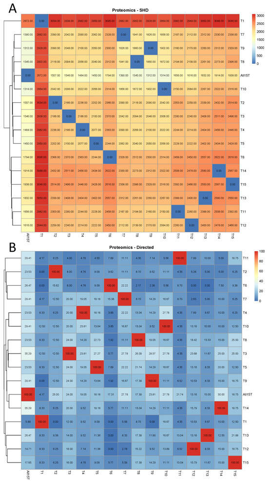
Figure 2.
Proteomic analysis. The comparison of each of the 16 CPDAGs (rows) to all 16 reference CPDAGs (columns) is displayed. Hierarchical clustering was performed by row. (A) SHDs, (B) The percentages of the directed edges in each of the reference causal structures that remained directed with the same direction in each of the 16 CPDAGs.
This was not the case, however, when the percentage of directed edges in each of the reference causal structures that remained directed with the same direction in each of the remaining causal structures was assessed (Figure 2B). In this case, it was observed that CPDAGs corresponding to the exclusion of tissues with similar biological functions did not cluster together. In addition, there was no CPDAG that demonstrated systematically high or low values of percentages of common directed edges to each of the reference CPDAGs, compared to all other CPDAGs. Still, the lowest percentage of commonly directed edges to the All15T CPDAG was observed in the case of T1 with 5.88% (Figure 2B), while the highest percentage was in the case of CPDAG T3 and T14 (35.29).
When the percentage of directed edges in each of the reference causal structures that either remained directed with the same direction or turned into bidirected in each of the remaining causal structures was assessed (Figure A2), the results were very similar to in the previous case (Figure 2B). More specifically, the CPDAGs corresponding to excluded tissues with similar biological functions did not cluster together and the lowest percentage of directed edges in the CPDAG All15T that either were retained or turned into bidirected was observed in the case of T1 with 29.41% (Figure A2). The highest percentage involved CPDAG T9 (61.76%) followed by CPDAG T3 (58.82%).
Numerical details regarding the metrics considered are displayed in Table A2. Similarly, as in the case of the transcriptomic analysis, it was observed that the number of directed edges in each reference CPDAG that changed direction was in almost all cases zero. Compared to the CPDAG All15T, only in the case of CPDAGs T2 and T8, there was observed one change in direction, while in all other cases, the direction changes were zero.
In the proteogenomic case, it is shown in Figure 3A that when the 1st tissue (“1st Bloom”) was removed from the combined database, the impact was the highest of all cases and CPDAG T1 exhibited by far the highest SHD among all CPDAGs, compared to ALL15T (3270). T1 exhibited the highest SHD to each of the CPDAGs when treated as a reference, compared to all other CPDAGs as well. The smallest SHD compared to the CPDAG ALL15T was observed in the case of CPDAG T9 (1654). These results are similar to the respective results in the proteomic analysis. Moreover, the CPDAGs corresponding to the exclusion of tissues 3–4, which are related to the fruiting stage, were clustered together in the heatmap (Figure 3A). Similarly, the CPDAGs T7–T10 that correspond to the four stem stages were also clustered close to each other. In addition, CPDAGs T11–T12 (corresponding to the tissues “Dormancy buds” and “Flower”), and T14–T15 (“Leaves”, “Young leaves”) were clustered together, respectively, as well (Figure 3A).
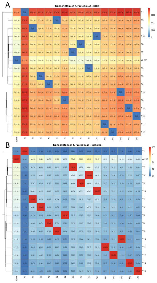
Figure 3.
Proteogenomic analysis. The comparison of each of the 16 CPDAGs (rows) to all 16 reference CPDAGs (columns) is displayed. Hierarchical clustering was performed by row. (A) SHDs, (B) The percentages of the directed edges in each of the reference causal structures that remained directed with the same direction in each of the 16 CPDAGs.
These results were observed as well when assessing the percentage of directed edges in each of the reference causal structures that retained their direction in each of the remaining causal structures (Figure 3B). In this case, the results were even more emphatical, since the CPDAGs T4–T6 (correspond to fruit stages), the CPDAGs T7–T10 (four stem stages), the CPDAGs T11–T13 (buds and flowers) and the CPDAGs T14–T15 (leaves) were also clustered together, respectively. (Figure 3B). On top of that, similarly to the assessment of SHD (Figure 3A), the CPDAG that exhibited the least similarity to all other reference CPDAGs was T1. Particularly, when compared to All15T, it exhibited a percentage of 25.19%, which was by far lower than any other CPDAG (the highest percentage was 52.89% and was observed in the cases of both T7 and T9).
Next, the percentage of directed edges in each of the reference causal structures that either remained directed with the same direction or turned into bidirected, in each of the remaining causal structures was assessed (Figure A3). The results were very similar to the previous case (Figure 3B) and the case when the SHD was assessed (Figure 3A). On top of the fact that CPDAGs corresponding to the exclusion of biologically similar tissues were clustered together, CPDAG T1 again exhibited the least similarity to all other reference CPDAGs. The lowest by far percentage of directed edges in the CPDAG All15T that either were retained or turned into bidirected was 46.74% (T1), while the highest was 70.80% followed by 70.62% (again involving T9 and T7, respectively).
Numerical details regarding the metrics considered are displayed in Table A3. In this case, it was observed that the number of directed edges in each reference CPDAG that changed direction received large numbers in almost all cases. When considering the CPDAG All15T as a reference, CPDAG T1 exhibited the highest number of direction changes (86), which additionally was the highest number of direction changes overall (Table A3).
4. Discussion
This study proposes a causal structure robustness assessment algorithm for single-omic or multiomics data involving plant tissues and demonstrates its application on a sweet cherry proteogenomic atlas. The robustness assessment of the causal structures based on the transcriptomic, proteomic, and combined proteogenomic datasets underscored that different tissues were revealed, in each case, to exhibit the highest impact when excluded from the corresponding databases. Notably, by excluding the tissues “Dormancy buds” and “Fruit 1st stage”, the causal structure based on the transcriptomic data was pronouncedly more influenced compared to the exclusion of the remaining tissues (based on the SHD, Figure 1A and the percentage of directed edges retained, Figure 1B, respectively). This could be attributed to the fact that while the transcriptional regulation in dormant buds is limited, during the transition from endodormancy to ecodormancy an explosion of transcription activity has been observed that clearly divided the ecodormancy from other dormancy stages in sweet cherries [44,45,46]. Similarly, the early stage of fruit development is characterized by elevated transcriptional activity due to continuous cell division that progressively decreases in the following stages [47,48]. Hence, the endorsement of transcriptional activity was observed.
On the other hand, in the case of both the proteomic and the proteogenomic analysis, it was shown that when the first tissue (“1st Bloom”) was excluded from the data, the impact inflicted on the causal structure was the highest compared to all other tissues (Figure 2A and Figure 3A,B). The high impact of the exclusion of the “1st Bloom” tissue was even more evident in the case of the proteogenomic analysis. This may be attributed to the fact that “1st Bloom” is related to protein abundance that clearly separates it from the remaining tissues. This was observed as well and discussed in a previous publication of our group [31], and also noticed in Arabidopsis thaliana where exclusive proteins were found in abundance at pollen, callus, seed and flower of the plant [49].
Moreover, it was expected that the CPDAGs corresponding to the exclusion of biologically similar tissues would be clustered together or close to each other. In particular, the CPDAGs corresponding to the tissues 3–5 related to the fruiting stage, the CPDAGs T7–T10, corresponding to the four stem stages, the CPDAGs T1–T13 corresponding to the tissues “Dormancy buds”, “Flower” and “Flower buds”, and the CPDAGs T14–T15 corresponding to the tissues “Leaves” and “Young leaves”. This expectation was based on the fact that the only thing that theoretically changes is the developmental stage and not the histological one. When assessing the clustering of the CPDAGs, based on their SHD to all other CPDAGs, and the percentage of common directed edges (or directed and directed that turned into bidirected) with all other CPDAGs, it was found that in the transcriptomic case, this expectation was not satisfied (Figure 1 and Figure A1). Indeed, in a transcriptomic analysis of quality changes during sweet cherry fruit development, the transcriptome of the organs has been found to exhibit strong differentiation depending on the developmental stage [50,51].
This expectation was satisfied, however, in the case of both the proteomic and the proteogenomic analysis, at least when considering the SHD as the metric to assess the causal structure differences (Figure 2A and Figure 3A). In the case that the hierarchical clustering was based on the percentage of the directed edges in each of the reference causal structures that remained directed with the same direction in each of the remaining CPDAGs, and on the percentage of the directed edges in each of the reference causal structures that either remained directed with the same direction, or turned into bidirected in each of the CPDAGs, it was found that this expectation was fulfilled only in the case of the proteogenomic analysis (Figure 3A,B). This is probably because the combined analysis of proteome and transcriptome managed to separate tissues belonging to other organs, by reducing the noise from analyzing the proteome or transcriptome alone.
The fact that the expectation of CPDAGs corresponding to the removal of tissues with similar biological function to be clustered together was satisfied, the best in the case of the proteogenomic analysis additionally implies that collecting and analyzing fewer tissue samples from an organ, when this is relevant or necessary, may be facilitated in case a combined proteogenomic analysis is considered. Namely, in the case of a proteogenomic analysis, opting to use fewer representative tissues of a specific organ is expected to result in a milder impact on the corresponding causal structure, compared to the case of the single omic analysis of the proteome or the transcriptome.
By an overall comparison of the percentages of the directed edges in each of the reference causal structures that remained directed with the same direction in each of the remaining 15 CPDAGs (Figure 1B, Figure 2B and Figure 3B), it can be clearly observed that they are much higher in the case of the proteogenomic analysis compared to the other two cases. Since the SHD as a metric cannot be employed to technically compare the results, because it is largely influenced by the complexity of the CPDAGs considered, which in the case of the proteogenomic analysis is much more pronounced (see Table A1, Table A2 and Table A3 in Appendix A for more details), the above result is indicative of obtaining more robust causal structures in the case of jointly employing the proteome and transcriptome databases. These results reinforce the importance of a multi-omics approach to capture the full breadth of biological processes [52,53,54].
Lastly, the biological implications of analyzing and assessing the robustness of the obtained causal structures concern the reliability of the biological interpretations that may emerge from these causal structures. Namely, a robustness analysis may further support the biological conclusions emerging from causal discovery and at the same time highlight hidden aspects in the data.
5. Conclusions
By employing the proposed algorithm to assess omic sweet cherry causal structures, it is showcased that specific tissues exhibited a strong impact when removed from the analysis. In the proteogenomic case, a similar impact was induced on the causal structures when biologically related tissues were excluded. This result was less pronounced in the proteomic analysis and especially in the transcriptomic analysis. This may be attributed to the distinctive biological features related to proteome and transcriptome. Moreover, causal structures based on single omic analyses were impacted to a larger extent, compared to proteogenomic analysis. Thus, this study reveals the importance of assessing the causal structure robustness, along with causal discovery, within the framework of omics data, and showcases the added advantages and perspective. Furthermore, while not questioning the importance of separately performing a transcriptomic or proteomic analysis, it provides valuable insight into the benefits of employing a proteogenomic analysis, further supporting the usage of multiomics analysis in research.
Author Contributions
Conceptualization, M.G. and T.M.; Data curation, M.G. and A.X.; Formal analysis, M.G. and T.M.; Investigation, M.G., M.M. and I.G.; Methodology, M.G. and T.M.; Project administration, T.M.; Resources, A.X.; Software, M.G.; Supervision, I.G. and T.M.; Validation, A.X., M.M. and I.G.; Visualization, M.G. and T.M.; Writing, original draft, M.G. and T.M.; Writing, review and editing, A.X., M.M., L.A., I.G. and T.M. All authors have read and agreed to the published version of the manuscript.
Funding
This research received no external funding.
Data Availability Statement
The transcript expression and protein abundances are available in the SweetBiOmics database (www.GrCherrydb.com, accessed on 1 September 2023).
Conflicts of Interest
The authors declare no conflict of interest.
Appendix A
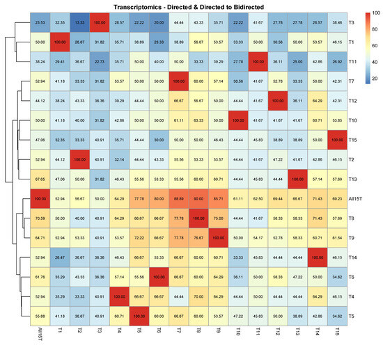
Figure A1.
Transcriptomic analysis. The comparison of each of the 16 CPDAGs (rows) to all 16 reference CPDAGs (columns) is displayed. Hierarchical clustering was performed by row. The percentages of the directed edges in each of the reference causal structures that either remained directed with the same direction or turned into bidirected in each of the 16 CPDAGs.
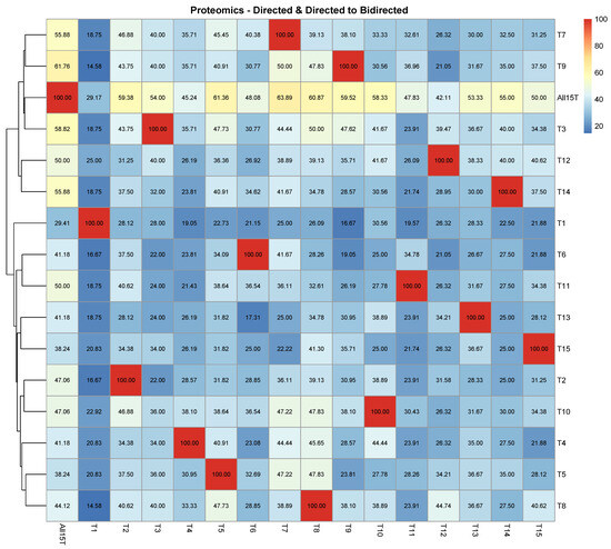
Figure A2.
Proteomic analysis. The comparison of each of the 16 CPDAGs (rows) to all 16 reference CPDAGs (columns) is displayed. Hierarchical clustering was performed by row. The percentages of the directed edges in each of the reference causal structures that either remained directed with the same direction or turned into bidirected in each of the 16 CPDAGs.
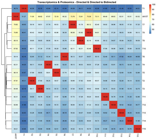
Figure A3.
Proteogenomic analysis. The comparison of each of the 16 CPDAGs (rows) to all 16 reference CPDAGs (columns) is displayed. Hierarchical clustering was performed by row. The percentages of the directed edges in each of the reference causal structures that either remained directed with the same direction or turned into bidirected in each of the 16 CPDAGs.

Table A1.
Transcriptomic analysis. The comparison of each of the 16 CPDAGs (rows) to all 16 reference CPDAGs (columns) is numerically displayed. The comparison is based on the structural Hamming distance (SHD) between each pair of CPDAGs, the number of bidirected edges in each reference CPDAG (columns) that remained bidirected (BiD) in each of the remaining CPDAGs (rows), the number of directed edges in each reference CPDAG (columns) that remained directed with the same direction (Dir) in each of the remaining CPDAGs (rows), the number of directed edges in each reference CPDAG (columns) that turned into bidirected (DtoB) in each of the remaining CPDAGs (rows), and the number of directed edges in each reference CPDAG (columns) that changed direction (DCh) in each of the remaining CPDAGs (rows).
| CPDAGs | Metrics | All15T | T1 | T2 | T3 | T4 | T5 | T6 | T7 | T8 | T9 | T10 | T11 | T12 | T13 | T14 | T15 |
|---|---|---|---|---|---|---|---|---|---|---|---|---|---|---|---|---|---|
| All15T | SHD | 0 | 1822 | 1818 | 1741 | 1268 | 882 | 1191 | 1334 | 1064 | 900 | 1644 | 2256 | 1540 | 1478 | 1772 | 1932 |
| BiD | 1125 | 669 | 677 | 690 | 803 | 907 | 804 | 780 | 841 | 890 | 700 | 553 | 732 | 761 | 661 | 625 | |
| Dir | 34 | 8 | 10 | 4 | 10 | 10 | 14 | 8 | 20 | 18 | 10 | 6 | 10 | 18 | 10 | 12 | |
| DtoB | 0 | 10 | 7 | 7 | 8 | 4 | 10 | 8 | 7 | 6 | 12 | 9 | 15 | 6 | 10 | 6 | |
| DCh | 0 | 0 | 0 | 1 | 0 | 0 | 1 | 0 | 0 | 0 | 0 | 0 | 0 | 0 | 0 | 0 | |
| T1 | SHD | 1822 | 0 | 2502 | 2604 | 2268 | 2074 | 2255 | 2312 | 2166 | 2074 | 2501 | 2900 | 2352 | 2352 | 2540 | 2570 |
| BiD | 669 | 1117 | 506 | 470 | 552 | 608 | 541 | 536 | 565 | 595 | 487 | 390 | 531 | 540 | 470 | 464 | |
| Dir | 8 | 34 | 6 | 2 | 2 | 4 | 2 | 4 | 10 | 10 | 8 | 4 | 6 | 8 | 6 | 6 | |
| DtoB | 9 | 0 | 2 | 5 | 8 | 3 | 5 | 3 | 7 | 5 | 4 | 8 | 5 | 10 | 9 | 6 | |
| DCh | 0 | 0 | 0 | 0 | 0 | 0 | 1 | 0 | 0 | 0 | 1 | 0 | 0 | 0 | 0 | 0 | |
| T2 | SHD | 1818 | 2502 | 0 | 2590 | 2238 | 2042 | 2259 | 2242 | 2118 | 2022 | 2458 | 2882 | 2436 | 2340 | 2550 | 2592 |
| BiD | 677 | 506 | 1131 | 482 | 567 | 623 | 546 | 561 | 584 | 615 | 502 | 402 | 515 | 551 | 474 | 465 | |
| Dir | 10 | 6 | 30 | 2 | 2 | 4 | 9 | 6 | 6 | 10 | 6 | 6 | 10 | 8 | 6 | 6 | |
| DtoB | 8 | 9 | 0 | 7 | 7 | 4 | 4 | 4 | 10 | 5 | 10 | 4 | 7 | 7 | 6 | 6 | |
| DCh | 0 | 0 | 0 | 0 | 0 | 0 | 1 | 0 | 0 | 0 | 0 | 0 | 0 | 0 | 0 | 0 | |
| T3 | SHD | 1741 | 2604 | 2590 | 0 | 2186 | 2042 | 2154 | 2191 | 2126 | 2022 | 2507 | 2810 | 2420 | 2334 | 2576 | 2582 |
| BiD | 690 | 470 | 482 | 1113 | 571 | 614 | 564 | 563 | 573 | 607 | 483 | 410 | 511 | 546 | 458 | 457 | |
| Dir | 4 | 2 | 2 | 22 | 4 | 2 | 2 | 2 | 4 | 4 | 2 | 2 | 4 | 4 | 2 | 4 | |
| DtoB | 4 | 9 | 2 | 0 | 4 | 2 | 4 | 6 | 9 | 6 | 6 | 8 | 6 | 6 | 6 | 6 | |
| DCh | 1 | 0 | 0 | 0 | 0 | 0 | 0 | 1 | 0 | 0 | 1 | 0 | 0 | 0 | 0 | 0 | |
| T4 | SHD | 1268 | 2268 | 2238 | 2186 | 0 | 1438 | 1730 | 1852 | 1696 | 1606 | 2102 | 2600 | 2106 | 2070 | 2250 | 2368 |
| BiD | 803 | 552 | 567 | 571 | 1110 | 760 | 664 | 646 | 676 | 707 | 579 | 459 | 586 | 607 | 534 | 510 | |
| Dir | 10 | 2 | 2 | 4 | 28 | 8 | 12 | 6 | 12 | 10 | 4 | 2 | 6 | 6 | 6 | 6 | |
| DtoB | 8 | 10 | 8 | 5 | 0 | 4 | 8 | 2 | 9 | 8 | 12 | 10 | 10 | 10 | 12 | 6 | |
| DCh | 0 | 0 | 0 | 0 | 0 | 0 | 0 | 0 | 0 | 0 | 0 | 0 | 0 | 0 | 0 | 0 | |
| T5 | SHD | 882 | 2074 | 2042 | 2042 | 1438 | 0 | 1457 | 1660 | 1490 | 1316 | 1898 | 2504 | 1832 | 1856 | 2068 | 2190 |
| BiD | 907 | 608 | 623 | 614 | 760 | 1127 | 740 | 700 | 737 | 787 | 638 | 490 | 662 | 668 | 589 | 562 | |
| Dir | 10 | 4 | 4 | 2 | 8 | 18 | 8 | 4 | 10 | 8 | 6 | 2 | 8 | 4 | 6 | 4 | |
| DtoB | 9 | 10 | 7 | 7 | 9 | 0 | 10 | 8 | 8 | 7 | 11 | 9 | 10 | 10 | 6 | 5 | |
| DCh | 0 | 0 | 0 | 0 | 0 | 0 | 1 | 0 | 0 | 0 | 0 | 0 | 0 | 0 | 0 | 0 | |
| T6 | SHD | 1191 | 2255 | 2259 | 2154 | 1730 | 1457 | 0 | 1834 | 1659 | 1481 | 2051 | 2622 | 2005 | 2031 | 2273 | 2429 |
| BiD | 804 | 541 | 546 | 564 | 664 | 740 | 1078 | 634 | 669 | 721 | 576 | 439 | 593 | 600 | 513 | 480 | |
| Dir | 14 | 2 | 9 | 2 | 12 | 8 | 30 | 8 | 10 | 12 | 4 | 6 | 10 | 8 | 6 | 4 | |
| DtoB | 7 | 10 | 4 | 6 | 4 | 2 | 0 | 4 | 8 | 6 | 9 | 6 | 11 | 9 | 8 | 5 | |
| DCh | 1 | 1 | 1 | 0 | 0 | 1 | 0 | 0 | 1 | 1 | 1 | 0 | 1 | 1 | 1 | 1 | |
| T7 | SHD | 1334 | 2312 | 2242 | 2191 | 1852 | 1660 | 1834 | 0 | 1768 | 1642 | 2132 | 2652 | 2139 | 2090 | 2194 | 2398 |
| BiD | 780 | 536 | 561 | 563 | 646 | 700 | 634 | 1102 | 653 | 693 | 569 | 443 | 570 | 599 | 545 | 497 | |
| Dir | 8 | 4 | 6 | 2 | 6 | 4 | 8 | 18 | 8 | 10 | 6 | 6 | 8 | 6 | 8 | 6 | |
| DtoB | 10 | 10 | 4 | 5 | 9 | 5 | 7 | 0 | 10 | 6 | 5 | 4 | 11 | 6 | 6 | 5 | |
| DCh | 0 | 0 | 0 | 1 | 0 | 0 | 0 | 0 | 0 | 0 | 0 | 0 | 1 | 0 | 0 | 0 | |
| T8 | SHD | 1064 | 2166 | 2118 | 2126 | 1696 | 1490 | 1659 | 1768 | 0 | 1318 | 1890 | 2482 | 1942 | 1928 | 2014 | 2242 |
| BiD | 841 | 565 | 584 | 573 | 676 | 737 | 669 | 653 | 1088 | 766 | 621 | 480 | 613 | 631 | 582 | 530 | |
| Dir | 20 | 10 | 6 | 4 | 12 | 10 | 10 | 8 | 30 | 16 | 10 | 4 | 10 | 14 | 12 | 12 | |
| DtoB | 4 | 7 | 6 | 5 | 6 | 2 | 10 | 6 | 0 | 5 | 6 | 6 | 11 | 7 | 8 | 3 | |
| DCh | 0 | 0 | 0 | 0 | 0 | 0 | 1 | 0 | 0 | 0 | 0 | 0 | 0 | 0 | 0 | 0 | |
| T9 | SHD | 900 | 2074 | 2022 | 2022 | 1606 | 1316 | 1481 | 1642 | 1318 | 0 | 1830 | 2412 | 1822 | 1804 | 2016 | 2182 |
| BiD | 890 | 595 | 615 | 607 | 707 | 787 | 721 | 693 | 766 | 1102 | 643 | 503 | 652 | 669 | 589 | 551 | |
| Dir | 18 | 10 | 10 | 4 | 10 | 8 | 12 | 10 | 16 | 28 | 8 | 6 | 10 | 14 | 10 | 10 | |
| DtoB | 4 | 8 | 6 | 5 | 5 | 5 | 8 | 4 | 7 | 0 | 10 | 7 | 9 | 7 | 7 | 6 | |
| DCh | 0 | 0 | 0 | 0 | 0 | 0 | 1 | 0 | 0 | 0 | 0 | 0 | 0 | 0 | 0 | 0 | |
| T10 | SHD | 1644 | 2501 | 2458 | 2507 | 2102 | 1898 | 2051 | 2132 | 1890 | 1830 | 0 | 2714 | 2335 | 2368 | 2356 | 2622 |
| BiD | 700 | 487 | 502 | 483 | 579 | 638 | 576 | 569 | 621 | 643 | 1091 | 425 | 520 | 525 | 502 | 436 | |
| Dir | 10 | 8 | 6 | 2 | 4 | 6 | 4 | 6 | 10 | 8 | 36 | 4 | 8 | 8 | 8 | 8 | |
| DtoB | 7 | 6 | 6 | 5 | 8 | 3 | 11 | 5 | 9 | 6 | 0 | 6 | 7 | 7 | 9 | 6 | |
| DCh | 0 | 1 | 0 | 1 | 0 | 0 | 1 | 0 | 0 | 0 | 0 | 0 | 1 | 0 | 0 | 0 | |
| T11 | SHD | 2256 | 2900 | 2882 | 2810 | 2600 | 2504 | 2622 | 2652 | 2482 | 2412 | 2714 | 0 | 2782 | 2684 | 2750 | 2827 |
| BiD | 553 | 390 | 402 | 410 | 459 | 490 | 439 | 443 | 480 | 503 | 425 | 1102 | 414 | 452 | 407 | 391 | |
| Dir | 6 | 4 | 6 | 2 | 2 | 2 | 6 | 6 | 4 | 6 | 4 | 24 | 6 | 4 | 4 | 4 | |
| DtoB | 7 | 6 | 5 | 3 | 8 | 7 | 6 | 3 | 6 | 5 | 6 | 0 | 7 | 5 | 8 | 3 | |
| DCh | 0 | 0 | 0 | 0 | 0 | 0 | 0 | 0 | 0 | 0 | 0 | 0 | 0 | 0 | 0 | 1 | |
| T12 | SHD | 1540 | 2352 | 2436 | 2420 | 2106 | 1832 | 2005 | 2139 | 1942 | 1822 | 2335 | 2782 | 0 | 2230 | 2336 | 2490 |
| BiD | 732 | 531 | 515 | 511 | 586 | 662 | 593 | 570 | 613 | 652 | 520 | 414 | 1104 | 566 | 512 | 477 | |
| Dir | 10 | 6 | 10 | 4 | 6 | 8 | 10 | 8 | 10 | 10 | 8 | 6 | 36 | 6 | 10 | 6 | |
| DtoB | 5 | 7 | 3 | 4 | 5 | 0 | 5 | 4 | 7 | 4 | 8 | 4 | 0 | 7 | 8 | 5 | |
| DCh | 0 | 0 | 0 | 0 | 0 | 0 | 1 | 1 | 0 | 0 | 1 | 0 | 0 | 0 | 0 | 0 | |
| T13 | SHD | 1478 | 2352 | 2340 | 2334 | 2070 | 1856 | 2031 | 2090 | 1928 | 1804 | 2368 | 2684 | 2230 | 0 | 2416 | 2338 |
| BiD | 761 | 540 | 551 | 546 | 607 | 668 | 600 | 599 | 631 | 669 | 525 | 452 | 566 | 1130 | 506 | 529 | |
| Dir | 18 | 8 | 8 | 4 | 6 | 4 | 8 | 6 | 14 | 14 | 8 | 4 | 6 | 36 | 10 | 12 | |
| DtoB | 5 | 8 | 7 | 3 | 7 | 6 | 8 | 4 | 4 | 3 | 8 | 7 | 10 | 0 | 6 | 3 | |
| DCh | 0 | 0 | 0 | 0 | 0 | 0 | 1 | 0 | 0 | 0 | 0 | 0 | 0 | 0 | 0 | 0 | |
| T14 | SHD | 1772 | 2540 | 2550 | 2576 | 2250 | 2068 | 2273 | 2194 | 2014 | 2016 | 2356 | 2750 | 2336 | 2416 | 0 | 2424 |
| BiD | 661 | 470 | 474 | 458 | 534 | 589 | 513 | 545 | 582 | 589 | 502 | 407 | 512 | 506 | 1080 | 481 | |
| Dir | 10 | 6 | 6 | 2 | 6 | 6 | 6 | 8 | 12 | 10 | 8 | 4 | 10 | 10 | 28 | 10 | |
| DtoB | 8 | 3 | 5 | 6 | 7 | 6 | 10 | 4 | 6 | 7 | 4 | 7 | 6 | 6 | 0 | 2 | |
| DCh | 0 | 0 | 0 | 0 | 0 | 0 | 1 | 0 | 0 | 0 | 0 | 0 | 0 | 0 | 0 | 0 | |
| T15 | SHD | 1932 | 2570 | 2592 | 2582 | 2368 | 2190 | 2429 | 2398 | 2242 | 2182 | 2622 | 2827 | 2490 | 2338 | 2424 | 0 |
| BiD | 625 | 464 | 465 | 457 | 510 | 562 | 480 | 497 | 530 | 551 | 436 | 391 | 477 | 529 | 481 | 1083 | |
| Dir | 12 | 6 | 6 | 4 | 6 | 4 | 4 | 6 | 12 | 10 | 8 | 4 | 6 | 12 | 10 | 26 | |
| DtoB | 4 | 5 | 4 | 5 | 4 | 4 | 5 | 3 | 3 | 3 | 8 | 7 | 8 | 2 | 4 | 0 | |
| DCh | 0 | 0 | 0 | 0 | 0 | 0 | 1 | 0 | 0 | 0 | 0 | 1 | 0 | 0 | 0 | 0 |
Table A2.
Proteomic analysis. The comparison of each of the 16 CPDAGs (rows) to all 16 reference CPDAGs (columns) is numerically displayed. The comparison is based on the structural Hamming distance (SHD) between each pair of CPDAGs, the number of bidirected edges in each reference CPDAG (columns) that remained bidirected (BiD) in each of the remaining CPDAGs (rows), the number of directed edges in each reference CPDAG (columns) that remained directed with the same direction (Dir) in each of the remaining CPDAGs (rows), the number of directed edges in each reference CPDAG (columns) that turned into bidirected (DtoB) in each of the remaining CPDAGs (rows), and the number of directed edges in each reference CPDAG (columns) that changed direction (DCh) in each of the remaining CPDAGs (rows).
| CPDAGs | Metrics | All15T | T1 | T2 | T3 | T4 | T5 | T6 | T7 | T8 | T9 | T10 | T11 | T12 | T13 | T14 | T15 |
|---|---|---|---|---|---|---|---|---|---|---|---|---|---|---|---|---|---|
| All15T | SHD | 0 | 2672 | 1557 | 1546 | 1484 | 1450 | 1794 | 1390 | 1345 | 1312 | 1314 | 1656 | 1616 | 1832 | 1914 | 1938 |
| BiD | 1049 | 399 | 669 | 645 | 680 | 679 | 599 | 679 | 707 | 717 | 712 | 632 | 646 | 585 | 572 | 563 | |
| Dir | 34 | 2 | 8 | 12 | 8 | 8 | 9 | 10 | 8 | 10 | 10 | 10 | 5 | 9 | 12 | 6 | |
| DtoB | 0 | 12 | 11 | 15 | 11 | 19 | 16 | 13 | 20 | 15 | 11 | 12 | 11 | 23 | 10 | 10 | |
| DCh | 0 | 0 | 1 | 0 | 0 | 0 | 0 | 0 | 1 | 0 | 0 | 0 | 0 | 0 | 0 | 0 | |
| T1 | SHD | 2672 | 0 | 3034 | 2938 | 2982 | 2950 | 3095 | 2882 | 2902 | 2928 | 2864 | 2982 | 2944 | 3050 | 3088 | 3046 |
| BiD | 399 | 1066 | 317 | 318 | 323 | 324 | 291 | 326 | 340 | 336 | 342 | 319 | 331 | 300 | 298 | 303 | |
| Dir | 2 | 48 | 0 | 6 | 4 | 4 | 0 | 2 | 4 | 0 | 6 | 2 | 4 | 4 | 4 | 4 | |
| DtoB | 8 | 0 | 9 | 8 | 4 | 6 | 11 | 7 | 8 | 7 | 5 | 7 | 6 | 13 | 5 | 3 | |
| DCh | 0 | 0 | 0 | 0 | 0 | 0 | 1 | 0 | 0 | 0 | 0 | 0 | 0 | 0 | 0 | 0 | |
| T2 | SHD | 1557 | 3034 | 0 | 2186 | 2236 | 2202 | 2366 | 2090 | 2118 | 2090 | 2042 | 2353 | 2259 | 2339 | 2432 | 2514 |
| BiD | 669 | 317 | 1062 | 498 | 500 | 502 | 466 | 514 | 524 | 535 | 537 | 467 | 495 | 471 | 453 | 427 | |
| Dir | 8 | 0 | 32 | 4 | 2 | 4 | 5 | 4 | 4 | 4 | 4 | 2 | 2 | 3 | 2 | 2 | |
| DtoB | 8 | 8 | 0 | 7 | 10 | 10 | 10 | 9 | 14 | 9 | 10 | 9 | 10 | 14 | 8 | 8 | |
| DCh | 1 | 0 | 0 | 0 | 0 | 0 | 0 | 0 | 0 | 0 | 0 | 1 | 1 | 1 | 0 | 0 | |
| T3 | SHD | 1546 | 2938 | 2186 | 0 | 2186 | 2100 | 2370 | 2042 | 2094 | 2048 | 2006 | 2280 | 2240 | 2408 | 2511 | 2496 |
| BiD | 645 | 318 | 498 | 1007 | 489 | 502 | 441 | 502 | 505 | 520 | 524 | 463 | 474 | 429 | 409 | 408 | |
| Dir | 12 | 6 | 4 | 50 | 10 | 12 | 3 | 10 | 12 | 12 | 10 | 2 | 9 | 7 | 10 | 8 | |
| DtoB | 8 | 3 | 10 | 0 | 5 | 9 | 13 | 6 | 11 | 8 | 5 | 9 | 6 | 15 | 6 | 3 | |
| DCh | 0 | 0 | 0 | 0 | 0 | 0 | 0 | 0 | 0 | 0 | 0 | 0 | 0 | 0 | 1 | 0 | |
| T4 | SHD | 1484 | 2982 | 2236 | 2186 | 0 | 2077 | 2363 | 2090 | 2056 | 2100 | 2022 | 2244 | 2214 | 2404 | 2456 | 2446 |
| BiD | 680 | 323 | 500 | 489 | 1040 | 524 | 459 | 506 | 530 | 525 | 535 | 488 | 499 | 444 | 440 | 437 | |
| Dir | 8 | 4 | 2 | 10 | 42 | 8 | 2 | 8 | 6 | 6 | 10 | 2 | 3 | 4 | 4 | 2 | |
| DtoB | 6 | 6 | 9 | 7 | 0 | 10 | 10 | 8 | 15 | 6 | 6 | 9 | 7 | 17 | 7 | 5 | |
| DCh | 0 | 0 | 0 | 0 | 0 | 1 | 1 | 0 | 0 | 0 | 0 | 0 | 0 | 0 | 0 | 0 | |
| T5 | SHD | 1450 | 2950 | 2202 | 2100 | 2077 | 0 | 2244 | 2062 | 2040 | 2050 | 2056 | 2228 | 2222 | 2402 | 2434 | 2428 |
| BiD | 679 | 324 | 502 | 502 | 524 | 1027 | 479 | 504 | 526 | 531 | 521 | 481 | 488 | 437 | 436 | 434 | |
| Dir | 8 | 4 | 4 | 12 | 8 | 44 | 4 | 8 | 10 | 6 | 6 | 2 | 5 | 5 | 8 | 4 | |
| DtoB | 5 | 6 | 8 | 6 | 5 | 0 | 13 | 9 | 12 | 4 | 4 | 11 | 8 | 17 | 6 | 5 | |
| DCh | 0 | 0 | 0 | 0 | 1 | 0 | 0 | 0 | 0 | 0 | 0 | 0 | 0 | 0 | 0 | 0 | |
| T6 | SHD | 1794 | 3095 | 2366 | 2370 | 2363 | 2244 | 0 | 2328 | 2312 | 2300 | 2314 | 2458 | 2450 | 2557 | 2622 | 2616 |
| BiD | 599 | 291 | 466 | 441 | 459 | 479 | 1033 | 443 | 466 | 473 | 459 | 427 | 437 | 406 | 393 | 393 | |
| Dir | 9 | 0 | 5 | 3 | 2 | 4 | 52 | 8 | 1 | 1 | 2 | 4 | 0 | 0 | 3 | 3 | |
| DtoB | 5 | 8 | 7 | 8 | 8 | 11 | 0 | 7 | 12 | 7 | 7 | 12 | 8 | 16 | 8 | 4 | |
| DCh | 0 | 1 | 0 | 0 | 1 | 0 | 0 | 0 | 0 | 0 | 0 | 0 | 0 | 1 | 0 | 0 | |
| T7 | SHD | 1390 | 2882 | 2090 | 2042 | 2090 | 2062 | 2328 | 0 | 1941 | 1826 | 1856 | 2187 | 2112 | 2312 | 2330 | 2338 |
| BiD | 679 | 326 | 514 | 502 | 506 | 504 | 443 | 1001 | 538 | 569 | 555 | 478 | 501 | 448 | 447 | 443 | |
| Dir | 10 | 2 | 4 | 10 | 8 | 8 | 8 | 36 | 4 | 6 | 6 | 4 | 1 | 3 | 4 | 2 | |
| DtoB | 9 | 7 | 11 | 10 | 7 | 12 | 13 | 0 | 14 | 10 | 6 | 11 | 9 | 15 | 9 | 8 | |
| DCh | 0 | 0 | 0 | 0 | 0 | 0 | 0 | 0 | 1 | 0 | 0 | 1 | 0 | 0 | 0 | 0 | |
| T8 | SHD | 1345 | 2902 | 2118 | 2094 | 2056 | 2040 | 2312 | 1941 | 0 | 1860 | 1872 | 2194 | 2139 | 2261 | 2273 | 2396 |
| BiD | 707 | 340 | 524 | 505 | 530 | 526 | 466 | 538 | 1033 | 578 | 566 | 495 | 510 | 476 | 481 | 443 | |
| Dir | 8 | 4 | 4 | 12 | 6 | 10 | 1 | 4 | 46 | 8 | 6 | 2 | 7 | 8 | 6 | 8 | |
| DtoB | 7 | 3 | 9 | 8 | 8 | 11 | 14 | 10 | 0 | 8 | 8 | 9 | 10 | 14 | 5 | 5 | |
| DCh | 1 | 0 | 0 | 0 | 0 | 0 | 0 | 1 | 0 | 0 | 0 | 0 | 1 | 1 | 1 | 0 | |
| T9 | SHD | 1312 | 2928 | 2090 | 2048 | 2100 | 2050 | 2300 | 1826 | 1860 | 0 | 1902 | 2160 | 2170 | 2260 | 2312 | 2329 |
| BiD | 717 | 336 | 535 | 520 | 525 | 531 | 473 | 569 | 578 | 1039 | 564 | 505 | 509 | 480 | 474 | 463 | |
| Dir | 10 | 0 | 4 | 12 | 6 | 6 | 1 | 6 | 8 | 42 | 4 | 3 | 4 | 5 | 6 | 6 | |
| DtoB | 11 | 7 | 10 | 8 | 9 | 12 | 15 | 12 | 14 | 0 | 7 | 14 | 4 | 14 | 8 | 6 | |
| DCh | 0 | 0 | 0 | 0 | 0 | 0 | 0 | 0 | 0 | 0 | 0 | 0 | 0 | 0 | 0 | 1 | |
| T10 | SHD | 1314 | 2864 | 2042 | 2006 | 2022 | 2056 | 2314 | 1856 | 1872 | 1902 | 0 | 2150 | 2084 | 2267 | 2322 | 2316 |
| BiD | 712 | 342 | 537 | 524 | 535 | 521 | 459 | 555 | 566 | 564 | 1024 | 500 | 521 | 469 | 463 | 460 | |
| Dir | 10 | 6 | 4 | 10 | 10 | 6 | 2 | 6 | 6 | 4 | 36 | 2 | 5 | 6 | 4 | 4 | |
| DtoB | 6 | 5 | 11 | 8 | 6 | 11 | 17 | 11 | 16 | 12 | 0 | 12 | 5 | 13 | 8 | 7 | |
| DCh | 0 | 0 | 0 | 0 | 0 | 0 | 0 | 0 | 0 | 0 | 0 | 0 | 0 | 1 | 0 | 0 | |
| T11 | SHD | 1656 | 2982 | 2353 | 2280 | 2244 | 2228 | 2458 | 2187 | 2194 | 2160 | 2150 | 0 | 2260 | 2388 | 2508 | 2392 |
| BiD | 632 | 319 | 467 | 463 | 488 | 481 | 427 | 478 | 495 | 505 | 500 | 1032 | 484 | 447 | 423 | 448 | |
| Dir | 10 | 2 | 2 | 2 | 2 | 2 | 4 | 4 | 2 | 3 | 2 | 46 | 3 | 6 | 2 | 6 | |
| DtoB | 7 | 7 | 11 | 10 | 7 | 15 | 15 | 9 | 13 | 8 | 8 | 0 | 7 | 13 | 9 | 5 | |
| DCh | 0 | 0 | 1 | 0 | 0 | 0 | 0 | 1 | 0 | 0 | 0 | 0 | 0 | 0 | 0 | 0 | |
| T12 | SHD | 1616 | 2944 | 2259 | 2240 | 2214 | 2222 | 2450 | 2112 | 2139 | 2170 | 2084 | 2260 | 0 | 2400 | 2478 | 2466 |
| BiD | 646 | 331 | 495 | 474 | 499 | 488 | 437 | 501 | 510 | 509 | 521 | 484 | 1043 | 444 | 433 | 432 | |
| Dir | 5 | 4 | 2 | 9 | 3 | 5 | 0 | 1 | 7 | 4 | 5 | 3 | 38 | 5 | 6 | 6 | |
| DtoB | 12 | 8 | 8 | 11 | 8 | 11 | 14 | 13 | 11 | 11 | 10 | 9 | 0 | 18 | 10 | 7 | |
| DCh | 0 | 0 | 1 | 0 | 0 | 0 | 0 | 0 | 1 | 0 | 0 | 0 | 0 | 0 | 0 | 0 | |
| T13 | SHD | 1832 | 3050 | 2339 | 2408 | 2404 | 2402 | 2557 | 2312 | 2261 | 2260 | 2267 | 2388 | 2400 | 0 | 2580 | 2550 |
| BiD | 585 | 300 | 471 | 429 | 444 | 437 | 406 | 448 | 476 | 480 | 469 | 447 | 444 | 1027 | 404 | 405 | |
| Dir | 9 | 4 | 3 | 7 | 4 | 5 | 0 | 3 | 8 | 5 | 6 | 6 | 5 | 60 | 5 | 7 | |
| DtoB | 5 | 5 | 6 | 5 | 7 | 9 | 9 | 6 | 8 | 8 | 8 | 5 | 8 | 0 | 5 | 2 | |
| DCh | 0 | 0 | 1 | 0 | 0 | 0 | 1 | 0 | 1 | 0 | 1 | 0 | 0 | 0 | 0 | 0 | |
| T14 | SHD | 1914 | 3088 | 2432 | 2511 | 2456 | 2434 | 2622 | 2330 | 2273 | 2312 | 2322 | 2508 | 2478 | 2580 | 0 | 2567 |
| BiD | 572 | 298 | 453 | 409 | 440 | 436 | 393 | 447 | 481 | 474 | 463 | 423 | 433 | 404 | 1044 | 408 | |
| Dir | 12 | 4 | 2 | 10 | 4 | 8 | 3 | 4 | 6 | 6 | 4 | 2 | 6 | 5 | 40 | 6 | |
| DtoB | 7 | 5 | 10 | 6 | 6 | 10 | 15 | 11 | 10 | 6 | 7 | 8 | 5 | 13 | 0 | 6 | |
| DCh | 0 | 0 | 0 | 1 | 0 | 0 | 0 | 0 | 1 | 0 | 0 | 0 | 0 | 0 | 0 | 1 | |
| T15 | SHD | 1938 | 3046 | 2514 | 2496 | 2446 | 2428 | 2616 | 2338 | 2396 | 2329 | 2316 | 2392 | 2466 | 2550 | 2567 | 0 |
| BiD | 563 | 303 | 427 | 408 | 437 | 434 | 393 | 443 | 443 | 463 | 460 | 448 | 432 | 405 | 408 | 1036 | |
| Dir | 6 | 4 | 2 | 8 | 2 | 4 | 3 | 2 | 8 | 6 | 4 | 6 | 6 | 7 | 6 | 32 | |
| DtoB | 7 | 6 | 9 | 9 | 9 | 10 | 10 | 6 | 11 | 9 | 5 | 4 | 4 | 15 | 4 | 0 | |
| DCh | 0 | 0 | 0 | 0 | 0 | 0 | 0 | 0 | 0 | 1 | 0 | 0 | 0 | 0 | 1 | 0 |
Table A3.
Proteogenomic analysis. The comparison of each of the 16 CPDAGs (rows) to all 16 reference CPDAGs (columns) is numerically displayed. The comparison is based on the structural Hamming distance (SHD) between each pair of CPDAGs, the number of bidirected edges in each reference CPDAG (columns) that remained bidirected (BiD) in each of the remaining CPDAGs (rows), the number of directed edges in each reference CPDAG (columns) that remained directed with the same direction (Dir) in each of the remaining CPDAGs (rows), the number of directed edges in each reference CPDAG (columns) that turned into bidirected (DtoB) in each of the remaining CPDAGs (rows), and the number of directed edges in each reference CPDAG (columns) that changed direction (DCh) in each of the remaining CPDAGs (rows).
| CPDAGs | Metrics | All15T | T1 | T2 | T3 | T4 | T5 | T6 | T7 | T8 | T9 | T10 | T11 | T12 | T13 | T14 | T15 |
|---|---|---|---|---|---|---|---|---|---|---|---|---|---|---|---|---|---|
| All15T | SHD | 0 | 3270 | 1879 | 1994 | 2110 | 1897 | 2288 | 1698 | 1711 | 1654 | 1807 | 2245 | 2185 | 2413 | 2344 | 2379 |
| BiD | 1444 | 784 | 1047 | 1029 | 1002 | 1037 | 967 | 1064 | 1084 | 1111 | 1049 | 960 | 988 | 940 | 957 | 954 | |
| Dir | 1072 | 270 | 524 | 512 | 462 | 493 | 437 | 567 | 542 | 567 | 531 | 448 | 461 | 445 | 423 | 400 | |
| DtoB | 0 | 216 | 151 | 145 | 166 | 182 | 192 | 161 | 139 | 118 | 157 | 193 | 152 | 166 | 160 | 178 | |
| DCh | 0 | 86 | 61 | 55 | 68 | 52 | 69 | 65 | 59 | 57 | 54 | 63 | 69 | 73 | 78 | 77 | |
| T1 | SHD | 3270 | 0 | 3660 | 3679 | 3713 | 3730 | 3875 | 3563 | 3549 | 3570 | 3609 | 3786 | 3733 | 3910 | 3903 | 3824 |
| BiD | 784 | 1509 | 718 | 723 | 712 | 720 | 683 | 725 | 736 | 753 | 722 | 700 | 718 | 672 | 666 | 688 | |
| Dir | 270 | 948 | 221 | 201 | 206 | 203 | 194 | 235 | 203 | 208 | 193 | 199 | 186 | 207 | 188 | 197 | |
| DtoB | 231 | 0 | 212 | 197 | 199 | 191 | 207 | 210 | 209 | 192 | 203 | 202 | 196 | 192 | 198 | 208 | |
| DCh | 86 | 0 | 58 | 78 | 63 | 65 | 62 | 68 | 65 | 69 | 84 | 64 | 69 | 72 | 69 | 56 | |
| T2 | SHD | 1879 | 3660 | 0 | 2654 | 2762 | 2574 | 2971 | 2479 | 2436 | 2439 | 2499 | 2878 | 2842 | 3008 | 3002 | 3008 |
| BiD | 1047 | 718 | 1488 | 908 | 893 | 927 | 845 | 929 | 953 | 960 | 929 | 858 | 876 | 831 | 827 | 843 | |
| Dir | 524 | 221 | 950 | 365 | 342 | 351 | 302 | 368 | 356 | 353 | 383 | 315 | 326 | 297 | 292 | 287 | |
| DtoB | 204 | 218 | 0 | 177 | 180 | 206 | 207 | 211 | 184 | 192 | 187 | 214 | 185 | 206 | 205 | 191 | |
| DCh | 61 | 58 | 0 | 59 | 60 | 51 | 72 | 80 | 74 | 64 | 56 | 72 | 58 | 72 | 60 | 74 | |
| T3 | SHD | 1994 | 3679 | 2654 | 0 | 2685 | 2741 | 2948 | 2605 | 2576 | 2567 | 2650 | 2915 | 2842 | 3097 | 3019 | 3026 |
| BiD | 1029 | 723 | 908 | 1468 | 912 | 887 | 867 | 896 | 924 | 937 | 892 | 848 | 873 | 814 | 829 | 834 | |
| Dir | 512 | 201 | 365 | 941 | 336 | 328 | 313 | 364 | 340 | 370 | 360 | 335 | 338 | 295 | 305 | 275 | |
| DtoB | 179 | 199 | 187 | 0 | 170 | 193 | 180 | 199 | 177 | 161 | 192 | 187 | 172 | 201 | 183 | 205 | |
| DCh | 55 | 78 | 59 | 0 | 62 | 51 | 56 | 65 | 65 | 61 | 56 | 56 | 53 | 66 | 68 | 63 | |
| T4 | SHD | 2110 | 3713 | 2762 | 2685 | 0 | 2677 | 3034 | 2606 | 2643 | 2619 | 2623 | 2960 | 2956 | 3124 | 3073 | 3107 |
| BiD | 1002 | 712 | 893 | 912 | 1483 | 891 | 837 | 912 | 913 | 931 | 913 | 846 | 850 | 819 | 823 | 826 | |
| Dir | 462 | 206 | 342 | 336 | 928 | 346 | 315 | 361 | 344 | 342 | 354 | 307 | 303 | 278 | 280 | 281 | |
| DtoB | 206 | 213 | 191 | 182 | 0 | 201 | 188 | 193 | 184 | 172 | 185 | 203 | 193 | 210 | 201 | 197 | |
| DCh | 68 | 63 | 60 | 62 | 0 | 60 | 63 | 77 | 59 | 66 | 52 | 64 | 66 | 72 | 63 | 61 | |
| T5 | SHD | 1897 | 3730 | 2574 | 2741 | 2677 | 0 | 2811 | 2535 | 2512 | 2533 | 2590 | 2849 | 2873 | 2995 | 2994 | 3092 |
| BiD | 1037 | 720 | 927 | 887 | 891 | 1492 | 867 | 906 | 926 | 937 | 903 | 854 | 862 | 838 | 832 | 818 | |
| Dir | 493 | 203 | 351 | 328 | 346 | 935 | 324 | 360 | 339 | 339 | 343 | 326 | 315 | 295 | 280 | 265 | |
| DtoB | 216 | 211 | 199 | 207 | 209 | 0 | 232 | 230 | 214 | 196 | 220 | 213 | 198 | 211 | 207 | 216 | |
| DCh | 52 | 65 | 51 | 51 | 60 | 0 | 55 | 63 | 53 | 55 | 48 | 54 | 54 | 62 | 63 | 57 | |
| T6 | SHD | 2288 | 3875 | 2971 | 2948 | 3034 | 2811 | 0 | 2778 | 2848 | 2790 | 2854 | 3098 | 3113 | 3328 | 3200 | 3253 |
| BiD | 967 | 683 | 845 | 867 | 837 | 867 | 1477 | 867 | 863 | 904 | 852 | 813 | 822 | 775 | 801 | 800 | |
| Dir | 437 | 194 | 302 | 313 | 315 | 324 | 963 | 357 | 336 | 345 | 329 | 306 | 277 | 263 | 265 | 258 | |
| DtoB | 197 | 206 | 201 | 168 | 180 | 195 | 0 | 197 | 183 | 151 | 190 | 200 | 184 | 197 | 187 | 193 | |
| DCh | 69 | 62 | 72 | 56 | 63 | 55 | 0 | 72 | 61 | 72 | 64 | 57 | 66 | 69 | 69 | 56 | |
| T7 | SHD | 1698 | 3563 | 2479 | 2605 | 2606 | 2535 | 2778 | 0 | 2262 | 2167 | 2358 | 2670 | 2669 | 2883 | 2804 | 2783 |
| BiD | 1064 | 725 | 929 | 896 | 912 | 906 | 867 | 1454 | 977 | 1004 | 939 | 879 | 898 | 842 | 861 | 871 | |
| Dir | 567 | 235 | 368 | 364 | 361 | 360 | 357 | 987 | 409 | 451 | 410 | 364 | 356 | 347 | 345 | 326 | |
| DtoB | 190 | 220 | 194 | 196 | 175 | 206 | 193 | 0 | 168 | 150 | 178 | 205 | 168 | 197 | 181 | 195 | |
| DCh | 65 | 68 | 80 | 65 | 77 | 63 | 72 | 0 | 59 | 57 | 60 | 69 | 70 | 66 | 59 | 68 | |
| T8 | SHD | 1711 | 3549 | 2436 | 2576 | 2643 | 2512 | 2848 | 2262 | 0 | 2231 | 2307 | 2704 | 2725 | 2875 | 2837 | 2807 |
| BiD | 1084 | 736 | 953 | 924 | 913 | 926 | 863 | 977 | 1475 | 1007 | 968 | 889 | 892 | 851 | 868 | 878 | |
| Dir | 542 | 203 | 356 | 340 | 344 | 339 | 336 | 409 | 934 | 404 | 397 | 340 | 315 | 317 | 296 | 319 | |
| DtoB | 188 | 234 | 204 | 195 | 184 | 214 | 201 | 198 | 0 | 161 | 174 | 201 | 188 | 213 | 202 | 196 | |
| DCh | 59 | 65 | 74 | 65 | 59 | 53 | 61 | 59 | 0 | 58 | 54 | 62 | 79 | 71 | 63 | 59 | |
| T9 | SHD | 1654 | 3570 | 2439 | 2567 | 2619 | 2533 | 2790 | 2167 | 2231 | 0 | 2280 | 2663 | 2663 | 2873 | 2780 | 2802 |
| BiD | 1111 | 753 | 960 | 937 | 931 | 937 | 904 | 1004 | 1007 | 1520 | 985 | 907 | 920 | 865 | 893 | 889 | |
| Dir | 567 | 208 | 353 | 370 | 342 | 339 | 345 | 451 | 404 | 909 | 415 | 347 | 327 | 311 | 342 | 310 | |
| DtoB | 192 | 232 | 221 | 194 | 203 | 231 | 198 | 201 | 193 | 0 | 193 | 222 | 200 | 228 | 191 | 219 | |
| DCh | 57 | 69 | 64 | 61 | 66 | 55 | 72 | 57 | 58 | 0 | 50 | 66 | 58 | 64 | 61 | 55 | |
| T10 | SHD | 1807 | 3609 | 2499 | 2650 | 2623 | 2590 | 2854 | 2358 | 2307 | 2280 | 0 | 2774 | 2776 | 2904 | 2854 | 2897 |
| BiD | 1049 | 722 | 929 | 892 | 913 | 903 | 852 | 939 | 968 | 985 | 1460 | 861 | 868 | 844 | 848 | 856 | |
| Dir | 531 | 193 | 383 | 360 | 354 | 343 | 329 | 410 | 397 | 415 | 941 | 359 | 329 | 315 | 317 | 297 | |
| DtoB | 194 | 227 | 188 | 180 | 175 | 202 | 207 | 203 | 185 | 162 | 0 | 197 | 195 | 205 | 197 | 196 | |
| DCh | 54 | 84 | 56 | 56 | 52 | 48 | 64 | 60 | 54 | 50 | 0 | 59 | 57 | 65 | 55 | 56 | |
| T11 | SHD | 2245 | 3786 | 2878 | 2915 | 2960 | 2849 | 3098 | 2670 | 2704 | 2663 | 2774 | 0 | 3021 | 3143 | 3101 | 3058 |
| BiD | 960 | 700 | 858 | 848 | 846 | 854 | 813 | 879 | 889 | 907 | 861 | 1473 | 826 | 805 | 817 | 828 | |
| Dir | 448 | 199 | 315 | 335 | 307 | 326 | 306 | 364 | 340 | 347 | 359 | 964 | 303 | 289 | 275 | 282 | |
| DtoB | 220 | 212 | 198 | 190 | 188 | 216 | 204 | 206 | 195 | 182 | 191 | 0 | 201 | 207 | 195 | 199 | |
| DCh | 63 | 64 | 72 | 56 | 64 | 54 | 57 | 69 | 62 | 66 | 59 | 0 | 59 | 59 | 65 | 62 | |
| T12 | SHD | 2185 | 3733 | 2842 | 2842 | 2956 | 2873 | 3113 | 2669 | 2725 | 2663 | 2776 | 3021 | 0 | 3196 | 3138 | 3072 |
| BiD | 988 | 718 | 876 | 873 | 850 | 862 | 822 | 898 | 892 | 920 | 868 | 826 | 1487 | 806 | 812 | 836 | |
| Dir | 461 | 186 | 326 | 338 | 303 | 315 | 277 | 356 | 315 | 327 | 329 | 303 | 920 | 300 | 265 | 262 | |
| DtoB | 211 | 211 | 197 | 182 | 187 | 206 | 211 | 205 | 200 | 194 | 201 | 206 | 0 | 186 | 196 | 200 | |
| DCh | 69 | 69 | 58 | 53 | 66 | 54 | 66 | 70 | 79 | 58 | 57 | 59 | 0 | 56 | 52 | 78 | |
| T13 | SHD | 2413 | 3910 | 3008 | 3097 | 3124 | 2995 | 3328 | 2883 | 2875 | 2873 | 2904 | 3143 | 3196 | 0 | 3299 | 3207 |
| BiD | 940 | 672 | 831 | 814 | 819 | 838 | 775 | 842 | 851 | 865 | 844 | 805 | 806 | 1470 | 771 | 805 | |
| Dir | 445 | 207 | 297 | 295 | 278 | 295 | 263 | 347 | 317 | 311 | 315 | 289 | 300 | 962 | 259 | 274 | |
| DtoB | 197 | 200 | 209 | 184 | 174 | 200 | 201 | 196 | 188 | 188 | 189 | 199 | 174 | 0 | 194 | 186 | |
| DCh | 73 | 72 | 72 | 66 | 72 | 62 | 69 | 66 | 71 | 64 | 65 | 59 | 56 | 0 | 67 | 61 | |
| T14 | SHD | 2344 | 3903 | 3002 | 3019 | 3073 | 2994 | 3200 | 2804 | 2837 | 2780 | 2854 | 3101 | 3138 | 3299 | 0 | 3169 |
| BiD | 957 | 666 | 827 | 829 | 823 | 832 | 801 | 861 | 868 | 893 | 848 | 817 | 812 | 771 | 1473 | 799 | |
| Dir | 423 | 188 | 292 | 305 | 280 | 280 | 265 | 345 | 296 | 342 | 317 | 275 | 265 | 259 | 918 | 266 | |
| DtoB | 204 | 211 | 213 | 181 | 184 | 212 | 202 | 200 | 190 | 167 | 198 | 200 | 199 | 205 | 0 | 207 | |
| DCh | 78 | 69 | 60 | 68 | 63 | 63 | 69 | 59 | 63 | 61 | 55 | 65 | 52 | 67 | 0 | 69 | |
| T15 | SHD | 2379 | 3824 | 3008 | 3026 | 3107 | 3092 | 3253 | 2783 | 2807 | 2802 | 2897 | 3058 | 3072 | 3207 | 3169 | 0 |
| BiD | 954 | 688 | 843 | 834 | 826 | 818 | 800 | 871 | 878 | 889 | 856 | 828 | 836 | 805 | 799 | 1503 | |
| Dir | 400 | 197 | 287 | 275 | 281 | 265 | 258 | 326 | 319 | 310 | 297 | 282 | 262 | 274 | 266 | 910 | |
| DtoB | 224 | 220 | 216 | 204 | 191 | 226 | 211 | 217 | 196 | 197 | 207 | 216 | 196 | 205 | 200 | 0 | |
| DCh | 77 | 56 | 74 | 63 | 61 | 57 | 56 | 68 | 59 | 55 | 56 | 62 | 78 | 61 | 69 | 0 |
References
- Liu, Y.; Beyer, A.; Aebersold, R. On the dependency of cellular protein levels on mRNA abundance. Cell 2016, 165, 535–550. [Google Scholar] [CrossRef] [PubMed]
- Buccitelli, C.; Selbach, M. mRNAs, proteins and the emerging principles of gene expression control. Nat. Rev. Genet. 2020, 21, 630–644. [Google Scholar] [CrossRef] [PubMed]
- Faulkner, S.; Dun, M.; Hondermarck, H. Proteogenomics: Emergence and promise. Cell. Mol. Life Sci. 2015, 72, 953–957. [Google Scholar] [CrossRef] [PubMed]
- Lazar, Ι.; Karcini, A.; Ahuja, S.; Estrada-Palma, C. Proteogenomic analysis of protein sequence alterations in breast cancer cells. Sci. Rep. 2019, 9, 10381. [Google Scholar] [CrossRef] [PubMed]
- Nesvizhskii, A. Proteogenomics: Concepts, applications and computational strategies. Nat. Methods 2014, 11, 1114–1125. [Google Scholar] [CrossRef] [PubMed]
- Low, Τ.; Mohtar, Μ.; Ang, Μ.; Jamal, R. Connecting Proteomics to Next-Generation Sequencing: Proteogenomics and Its Current Applications in Biology. Proteomics 2019, 19, 1800235. [Google Scholar] [CrossRef] [PubMed]
- Song, Y.C.; Das, D.; Zhang, Y.; Chen, M.X.; Fernie, A.R.; Zhu, F.Y.; Han, J. Proteogenomics-based functional genome research: Approaches, applications, and perspectives in plants. Trends Biotechnol. 2023, 41, 1532–1548. [Google Scholar] [CrossRef] [PubMed]
- Wang, P.; Wu, X.; Shi, Z.; Tao, S.; Liu, Z.; Qi, K.; Xie, Z.; Qiao, X.; Gu, C.; Yin, H.; et al. A large-scale proteogenomic atlas of pear. Mol. Plant 2023, 16, 599–615. [Google Scholar] [CrossRef]
- Chen, M.X.; Zhu, F.; Gao, B.; Ma, K.; Zhang, Y.; Fernie, A.; Chen, X.; Dai, L.; Ye, N.H.; Zhang, X.; et al. Full-length transcript-based proteogenomics of rice improves its genome and proteome annotation. Plant Physiol. 2020, 182, 1510–1526. [Google Scholar] [CrossRef]
- Dhar, Y.V.; Asif, M.H. Genome and transcriptome-wide study of carbamoyltransferase genes in major fleshy fruits: A multi-omics study of evolution and functional significance. Front. Plant Sci. 2022, 13, 994159. [Google Scholar] [CrossRef]
- Li, J.; Liu, L.; Le, T.D. Practical Approaches to Causal Relationship Exploration; Springer: Berlin/Heidelberg, Germany, 2015. [Google Scholar]
- Gąsior, J.; Młyńczak, M.; Williams, C.; Popłonyk, A.; Kowalska, D.; Giezek, P.; Werner, B. The discovery of a data-driven causal diagram of sport participation in children and adolescents with heart disease: A pilot study. Front. Cardiovasc. Med. 2023, 10, 1247122. [Google Scholar] [CrossRef] [PubMed]
- Krethong, P.; Jirapaet, V.; Jitpanya, C.; Sloan, R. A causal model of health-related quality of life in Thai patients with heart-failure. J. Nurs. Scholarsh. 2008, 40, 254–260. [Google Scholar] [CrossRef] [PubMed]
- Tangkawanich, T.; Yunibhand, J.; Thanasilp, S.; Magilvy, K. Causal model of health: Health-related quality of life in people living with HIV/AIDS in the northern region of Thailand. Nurs. Health Sci. 2008, 10, 216–221. [Google Scholar] [CrossRef]
- Raghu, V.K.; Zhao, W.; Pu, J.; Leader, J.; Wang, R.; Herman, J.; Yuan, J.; Benos, P.; Wilson, D. Feasibility of lung cancer prediction from low-dose CT scan and smoking factors using causal models. Thorax 2019, 74, 643–649. [Google Scholar] [CrossRef]
- Shen, X.; Ma, S.; Vemuri, P.; Simon, G. Challenges and opportunities with causal discovery algorithms: Application to Alzheimer’s pathophysiology. Sci. Rep. 2020, 10, 2975. [Google Scholar] [CrossRef]
- Piccininni, M.; Konigorski, S.; Rohmann, J.; Kurth, T. Directed acyclic graphs and causal thinking in clinical risk prediction modeling. BMC Med. Res. Methodol. 2020, 20, 179. [Google Scholar] [CrossRef]
- Neto, E.; Ferrara, C.; Attie, A.; Yandell, B. Inferring causal phenotype networks from segregating populations. Genetics 2008, 179, 1089–1100. [Google Scholar] [CrossRef]
- Neto, E.; Keller, M.; Attie, A.; Yandell, B. Causal graphical models in systems genetics: A unified framework for joint inference of causal network and genetic architecture for correlated phenotypes. Ann. Appl. Stat. 2010, 4, 320. [Google Scholar]
- Zhang, X.; Zhao, X.; He, K.; Lu, L.; Cao, Y.; Liu, J.; Hao, J.; Liu, Z.; Chen, L. Inferring gene regulatory networks from gene expression data by path consistency algorithm based on conditional mutual information. Bioinformatics 2012, 28, 98–104. [Google Scholar] [CrossRef]
- Wu, H.; Liu, X. Dynamic bayesian networks modeling for inferring genetic regulatory networks by search strategy: Comparison between greedy hill climbing and mcmc methods. Int. J. Comput. Inf. Eng. 2008, 2, 2585–2595. [Google Scholar]
- Vasimuddin, M.; Aluru, S. Parallel exact dynamic bayesian network structure learning with application to gene networks. In Proceedings of the 2017 IEEE 24th International Conference on High Performance Computing (HiPC), Jaipur, India, 18–21 December 2017. [Google Scholar]
- Wille, A.; Zimmermann, P.; Vranová, E.; Fürholz, A.; Laule, O.; Bleuler, S.; Bühlmann, P. Sparse graphical Gaussian modeling of the isoprenoid gene network in Arabidopsis thaliana. Genome Biol. 2004, 5, R92. [Google Scholar] [CrossRef] [PubMed]
- Yu, J.; Smith, V.; Wang, P.; Hartemink, A.; Jarvis, E. Advances to Bayesian network inference for generating causal networks from observational biological data. Bioinformatics 2004, 20, 3594–3603. [Google Scholar] [CrossRef] [PubMed]
- Ram, R.; Chetty, M. A markov-blanket-based model for gene regulatory network inference. IEEE/ACM Trans. Comput. Biol. Bioinform. 2009, 8, 353–367. [Google Scholar] [CrossRef] [PubMed]
- Schadt, E.; Lamb, J.; Yang, X.; Zhu, J.; Edwards, S.; GuhaThakurta, D.; Lusis, A. An integrative genomics approach to infer causal associations between gene expression and disease. Nat. Genet. 2005, 37, 710–717. [Google Scholar] [CrossRef] [PubMed]
- Glymour, C.; Zhang, K.; Spirtes, P. Review of causal discovery methods based on graphical models. Front. Genet. 2019, 10, 524. [Google Scholar] [CrossRef]
- Skodra, C.; Michailidis, M.; Moysiadis, T.; Stamatakis, G.; Ganopoulou, M.; Adamakis, I.; Angelis, E.; Ganopoulos, I.; Tanou, G.; Samiotaki, M.; et al. Disclosing the molecular basis of salinity priming in olive trees using proteogenomic model discovery. Plant Physiol. 2022, 191, 1913–1933. [Google Scholar] [CrossRef]
- Boutsika, A.; Michailidis, M.; Ganopoulou, M.; Dalakouras, A.; Skodra, C.; Xanthopoulou, A.; Stamatakis, G.; Samiotaki, M.; Tanou, G.; Moysiadis, T.; et al. A wide foodomics approach coupled with metagenomics elucidates the enviromental signature of potatoes. iScience 2023, 26, 105917. [Google Scholar] [CrossRef]
- Ganopoulou, M.; Michailidis, M.; Angelis, L.; Ganopoulos, I.; Molassiotis, A.; Xanthopoulou, A.; Moysiadis, T. Could Causal Discovery in Proteogenomics Assist in Understanding Gene–Protein Relations? A Perennial Fruit Tree Case Study Using Sweet Cherry as a Model. Cells 2021, 11, 92. [Google Scholar] [CrossRef]
- Xanthopoulou, A.; Moysiadis, T.; Bazakos, C.; Karagiannis, E.; Karamichali, I.; Stamatakis, G.; Tanou, G. The perennial fruit tree proteogenomics atlas: A spatial map of the sweet cherry proteome and transcriptome. Plant J. 2022, 109, 1319–1336. [Google Scholar] [CrossRef]
- Alkio, M.; Jonas, U.; Declercq, M.; Van Nocker, S.; Knoche, M. Transcriptional dynamics of the developing sweet cherry (Prunus avium L.) fruit: Sequencing, annotation and expression profiling of exocarp-associated genes. Hortic. Res. 2014, 1, 11. [Google Scholar] [CrossRef]
- Berni, R.; Charton, S.; Planchon, S.; Romi, M.; Cantini, C.; Guerriero, G. Molecular investigation of Tuscan sweet cherries sampled over three years: Gene expression analysis coupled to metabolomics and proteomics. Hortic. Res. 2021, 8, 12. [Google Scholar] [CrossRef] [PubMed]
- Karagiannis, E.; Sarrou, E.; Michailidis, M.; Tanou, G.; Ganopoulos, I.; Bazakos, C.; Molassiotis, A. Fruit quality trait discovery and metabolic profiling in sweet cherry genebank collection in Greece. Food Chem. 2021, 342, 128315. [Google Scholar] [CrossRef] [PubMed]
- Michailidis, M.; Karagiannis, E.; Tanou, G.; Samiotaki, M.; Tsiolas, G.; Sarrou, E.; Molassiotis, A. Novel insights into the calcium action in cherry fruit development revealed by high-throughput mapping. Plant Mol. Biol. 2020, 104, 597–614. [Google Scholar] [CrossRef] [PubMed]
- Ganopoulou, M.; Moysiadis, T.; Gounaris, A.; Mittas, N.; Chatzopoulou, F.; Chatzidimitriou, D.; Sianos, G.; Vizirianakis, I.S.; Angelis, L. Single Nucleotide Polymorphisms’ Causal Structure Robustness within Coronary Artery Disease Patients. Biology 2023, 12, 709. [Google Scholar] [CrossRef] [PubMed]
- Langfelder, P.; Horvath, S. WGCNA: An R package for weighted correlation network analysis. BMC Bioinform. 2008, 9, 559. [Google Scholar] [CrossRef]
- Pearl, J. Causal diagrams for empirical research. Biometrika 1995, 82, 669–688. [Google Scholar] [CrossRef]
- Nagarajan, R.; Scutari, M.; Lèbre, S. Bayesian Networks in R; Springer: Berlin/Heidelberg, Germany, 2013; Volume 122, pp. 125–127. [Google Scholar]
- Tsamardinos, I.; Brown, L.; Aliferis, C. The max-min hill-climbing Bayesian network structure learning algorithm. Mach. Learn. 2006, 65, 31–78. [Google Scholar] [CrossRef]
- Neopolitan, R.E. Learning Bayesian Networks; Prentice Hall: Hoboken, NJ, USA, 2003. [Google Scholar]
- Spirtes, P.; Glymour, C.C.; Scheines, R. Causation, Prediction, and Search, 2nd ed.; The MIT Press: Cambridge, MA, USA, 2000. [Google Scholar]
- Tsagris, M.; Bordoudakis, G.; Lagani, V.; Tsamardinos, I. Constraint-based causal discovery with mixed data. Int. J. Data Sci. Anal. 2018, 6, 19–40. [Google Scholar] [CrossRef]
- Villar, L.; Lienqueo, I.; Llanes, A.; Rojas, P.; Perez, J.; Correa, F.; Sagredo, B.; Masciarelli, O.; Luna, V.; Almada, R. Comparative transcriptomic analysis reveals novel roles of transcription factors and hormones during the flowering induction and floral bud differentiation in sweet cherry trees (Prunus avium L. cv. Bing). PLoS ONE 2020, 15, e0230110. [Google Scholar] [CrossRef]
- Vimont, N.; Fouche, M.; Campoy, J.A.; Tong, M.; Arkoun, M.; Yvin, J.C.; Wigge, A.; Dirlewanger, E.; Cortijo, S.; Wenden, B. From bud formation to flowering: Transcriptomic state defines the cherry developmental phases of sweet cherry bud dormancy. BMC Genom. 2019, 20, 974. [Google Scholar] [CrossRef]
- Rothkegel, K.; Sandoval, P.; Soto, E.; Ulloa, L.; Riveros, A.; Lillo-Carmona, V.; Cáceres-Molina, J.; Almeida, A.; Meneses, C. Dormant but active: Chilling accumulation modulates the epigenome and transcriptome of Prunus avium during bud dormancy. Front. Plant Sci. 2020, 11, 1115. [Google Scholar] [CrossRef] [PubMed]
- Yang, H.; Tian, C.; Ji, S.; Ni, F.; Fan, X.; Yang, Y.; Sun, C.; Gong, H.; Zhang, A. Integrative analyses of metabolome and transcriptome reveals metabolomic variations and candidate genes involved in sweet cherry (Prunus avium L.) fruit quality during development and ripening. PLoS ONE 2021, 16, e0260004. [Google Scholar] [CrossRef] [PubMed]
- Michailidis, M.; Bazakos, C.; Kollaros, M.; Adamakis, I.D.S.; Ganopoulos, I.; Molassiotis, A.; Tanou, G. Boron stimulates fruit formation and reprograms developmental metabolism in sweet cherry. Physiol. Plant. 2023, 175, 13946. [Google Scholar] [CrossRef] [PubMed]
- Mergner, J.; Frejno, M.; List, M.; Papacek, M.; Chen, X.; Chaudhary, A.; Samaras, P.; Richter, S.; Shikata, H.; Messerer, M.; et al. Mass-spectrometry-based draft of the Arabidopsis proteome. Nature 2020, 579, 409–414. [Google Scholar] [CrossRef] [PubMed]
- Zhang, Y.; Chen, C.; Cui, Y.; Du, Q.; Tang, W.; Yang, W.; Kou, G.; Tang, W.; Chen, H.; Gong, R. Potential regulatory genes of light induced anthocyanin accumulation in sweet cherry identified by combining transcriptome and metabolome analysis. Front. Plant Sci. 2023, 14, 1238624. [Google Scholar] [CrossRef] [PubMed]
- Chen, C.; Chen, H.; Yang, W.; Li, J.; Tang, W.; Gong, R. Transcriptomic and metabolomic analysis of quality changes during sweet cherry fruit development and mining of related genes. Int. J. Mol. Sci. 2022, 23, 7402. [Google Scholar] [CrossRef]
- Sirangelo, T. Multi-omics approaches in the study of plants. Int. J. Adv. Res. Bot. 2019, 5, 1–7. [Google Scholar]
- Hasin, Y.; Seldin, M.; Lusis, A. Multi-omics approaches to disease. Genome Biol. 2017, 18, 83. [Google Scholar] [CrossRef]
- Mahmood, U.; Li, X.; Fan, Y.; Chang, W.; Niu, Y.; Li, J.; Qu, C.; Lu, K. Multi-omics revolution to promote plant breeding efficiency. Front. Plant Sci. 2022, 13, 1062952. [Google Scholar] [CrossRef]
Disclaimer/Publisher’s Note: The statements, opinions and data contained in all publications are solely those of the individual author(s) and contributor(s) and not of MDPI and/or the editor(s). MDPI and/or the editor(s) disclaim responsibility for any injury to people or property resulting from any ideas, methods, instructions or products referred to in the content. |
© 2023 by the authors. Licensee MDPI, Basel, Switzerland. This article is an open access article distributed under the terms and conditions of the Creative Commons Attribution (CC BY) license (https://creativecommons.org/licenses/by/4.0/).