Development and Optimization of a Chamber System Applied to Maize Net Ecosystem Carbon Exchange Measurements

Abstract

Net ecosystem carbon exchange (NEE) in agricultural land represents a significant source of global greenhouse gas (GHG) emissions. While there are various tools for measuring NEE in agricultural fields, the chamber method remains the sole tool at the plot scale. In this research, we evaluated the NEE of maize plants at the nodulation stage using the flow-through chamber method. Many existing flow-through chamber systems directly introduce gases, leading to collisions with plants and subsequent turbulence inside the chamber. Turbulence can extend the time required to achieve a steady state. We modified the traditional flow-through chamber design to minimize turbulence in the measurement zone. Our modifications were validated by modeling the chamber and maize plants and by conducting fluid simulation experiments. In the analysis of our comparative field measurements between the two chamber designs, the use of the improved system notably shortened the time required to reach the steady state, increased the measurement frequency, and reduced the influence of changing environmental factors on the readings. Enhancing the measurement frequency is crucial for ensuring long-term accuracy. By reducing turbulence in the chamber, we anticipate improvements in the precision of NEE measurements in agricultural research, which could significantly contribute to an accurate assessment of the global carbon cycle.

1. Introduction

With the increasing prominence of various climate and environmental problems such as the greenhouse effect and the objective of evaluating carbon sources and sinks in international climate negotiations, carbon cycle issues are receiving increasing attention, and greenhouse gases (GHGs) such as carbon dioxide (CO₂), methane (CH₄), and nitrous oxide (N₂O) emitted from terrestrial environments are considered the main factors contributing to global warming. Approximately 13% of global anthropogenic GHGs are associated with GHGs originating from soil and agricultural inputs [1,2]. Identifying ecosystems in which agricultural lands function as carbon sinks (net CO₂ uptake) or sources (net CO₂ release) requires accurate measurement of net ecosystem exchange (NEE) CO₂ fluxes, i.e., the net fluxes between CO₂ uptake via photosynthesis and CO₂ loss via plant and soil respiration [3,4]. Monitoring the net CO₂ gas exchange of ecosystems is a key tool for evaluating biosphere–atmosphere feedback in climate systems.

Field measurements of greenhouse gases provide the basis for estimating greenhouse gas fluxes and a means of evaluating potential mitigation responses. There are several methods for measuring GHG fluxes in ecosystems, and the two most important methods are chamber-based and micrometeorological methods [5].

Micrometeorological methods, particularly the eddy covariance technique, are widely used in ecological studies [6,7]. Micrometeorological measurements, such as eddy covariance measurements, fully account for atmospheric exchange properties and capture all flux components that contribute to gas exchange between the canopy and the atmosphere. The use of the eddy covariance method necessitates extensive, uniform terrain, thereby limiting its use in experiments conducted over small areas [8]. Farmland cultivation is unevenly distributed in many countries, and the eddy covariance technique has achieved precise measurement results in large-scale agricultural environments [9,10]; however, it is relatively challenging to measure fluxes using eddy covariance techniques under smaller-area farmland conditions due to issues such as measurement boundaries [11]. At the same time, eddy covariance techniques are costly and unsuitable for widespread placement and thus are not conducive to accurate, large-scale, small-area monitoring.

The chamber method, due to its cost-effectiveness, size flexibility, and suitability for small scales, addresses these limitations [12,13], which are currently prevalent in soil respiration and ecosystem gas flux measurements [14,15,16,17,18]. The chamber method can be subdivided into closed chambers (also known as transient or nonstationary chambers) and flow-through chambers (also known as steady-state chambers) based on the measurement method [19]. Closed flux chambers can be used to calculate gas fluxes by measuring the change in the gas concentration over a given period in a confined space, in conjunction with the appropriate model [20]; flow-through chambers aim to calculate gas fluxes based on the difference in the concentration of gases entering and exiting the chamber [21]. The closed gas chamber method is now widely used for soil respiration measurements, where its reliability has been distinctly demonstrated [14,22,23]. In some studies, closed flux chambers have been applied to the measurement of NEE in ecosystems [4,24,25]; however, when measuring NEE using this method, the accumulating concentration in the flux chamber impacts the crops. The use of flow-through chambers overcomes the above problems associated with concentration buildup by using the difference in the gas concentration between the gas inlet and outlet after reaching a steady state to calculate gas fluxes, and the environmental factors inside the chamber are kept at the same level as those outside the chamber [15].

When transitioning from soil to agroecosystem measurements, chambers were enlarged to fully encompass plants, resulting in a minimal, almost negligible, pressure difference between the chamber interior and exterior. Typically, the design of gas exchange systems varies based on the research objectives [26]. It has been determined that flow-through chambers with different shapes, sampling flow rates, and internal gas circulation conditions can impose different effects on the measured object under the same environmental conditions due to the altered mass transfer characteristics inside the chamber, leading to different measurement results; this is one of the reasons for the discrepancy in measurement results between the micrometeorological and gas-chamber methods when measuring carbon fluxes [26]. Large gas-chamber systems for plant gas flux measurements have proven their reliability and are widely used for different measurements [27]. Thus, uncertainties persist in farmland flux measurements using flow-through chambers, with limited studies focused on enhancing their measurement performance.

In this study, we deployed a flow-through chamber to measure the net ecosystem carbon exchange (NEE) of maize plants at the elongation stage. Recognizing challenges such as internal chamber turbulence and potential measurement biases due to pressure differences, we aimed to refine the chamber design. Our approach involved rigorous modeling, simulation, and field measurements. Furthermore, our design could achieve an effective transition of the internal airflow to a laminar or low-turbulence state, promoting swifter attainment of a steady state. This innovative design was verified using computational fluid dynamic (CFD) techniques. The combined simulation and field test results demonstrated the enhanced performance of our modified chamber in capturing NEE of the representative farmland ecosystem.

2. Materials and Methods

2.1. Theory of the Flow-through Chamber and Flux Calculation

The gas in the flow-through chamber is forced by a tool such as an air pump. The flux of a particular gas (CO₂ in this experiment) in the chamber can be measured based on the difference in the gas concentration between the inlet and outlet ports.

This procedure can be described by Equation (1) [28]:

$$V\times \frac{d{C}_{out}}{dt}=A\times F_{co2}-Q\times \left[{C_{out}}_{}-C_{in}\right]$$

(1)

where V (m³) denotes the volume of the chamber, $\frac{d{C}_{out}}{dt}$ (mol m⁻³ s⁻¹) denotes the rate of change in carbon dioxide concentration within the chamber, A (m²) denotes the area of the soil and crop covered by the chamber, $F_{co2}$ (mol m⁻² s⁻¹) is the value of the carbon dioxide flux in the chamber, and Q (m³ s⁻¹) is the air flow rate into the chamber. C_out (mol m⁻³) and C_in (mol m⁻³) are the CO₂ gas mixing ratios of the gas inside the chamber and the gas flowing into the chamber, respectively. In a closed chamber system, the value of Q inside the chamber is zero. Moreover, the flow-through chamber continues to force external gas into the chamber throughout the measurement process. When it is sufficiently large, the difference between the concentration of gas flowing out of the chamber and that of the trace gas flowing into the chamber remains unchanged, and the chamber reaches a steady state in which the temporal derivative and temporal correlation in Equation (1) disappear [28,29]. Therefore, under equilibrium conditions, the mass budget equation for the flow-through chamber can be simplified and rearranged as Equation (2) [24]:

$$F_{co2}=\frac{Q}{A}\times \left(C_{out}-C_{in}\right)$$

(2)

According to Equation (2), the flux can be calculated as the product of the difference in carbon dioxide gas concentration between the inlet and outlet after a steady state is reached and the gas flow rate of the extracted gas.

2.2. Chamber Design

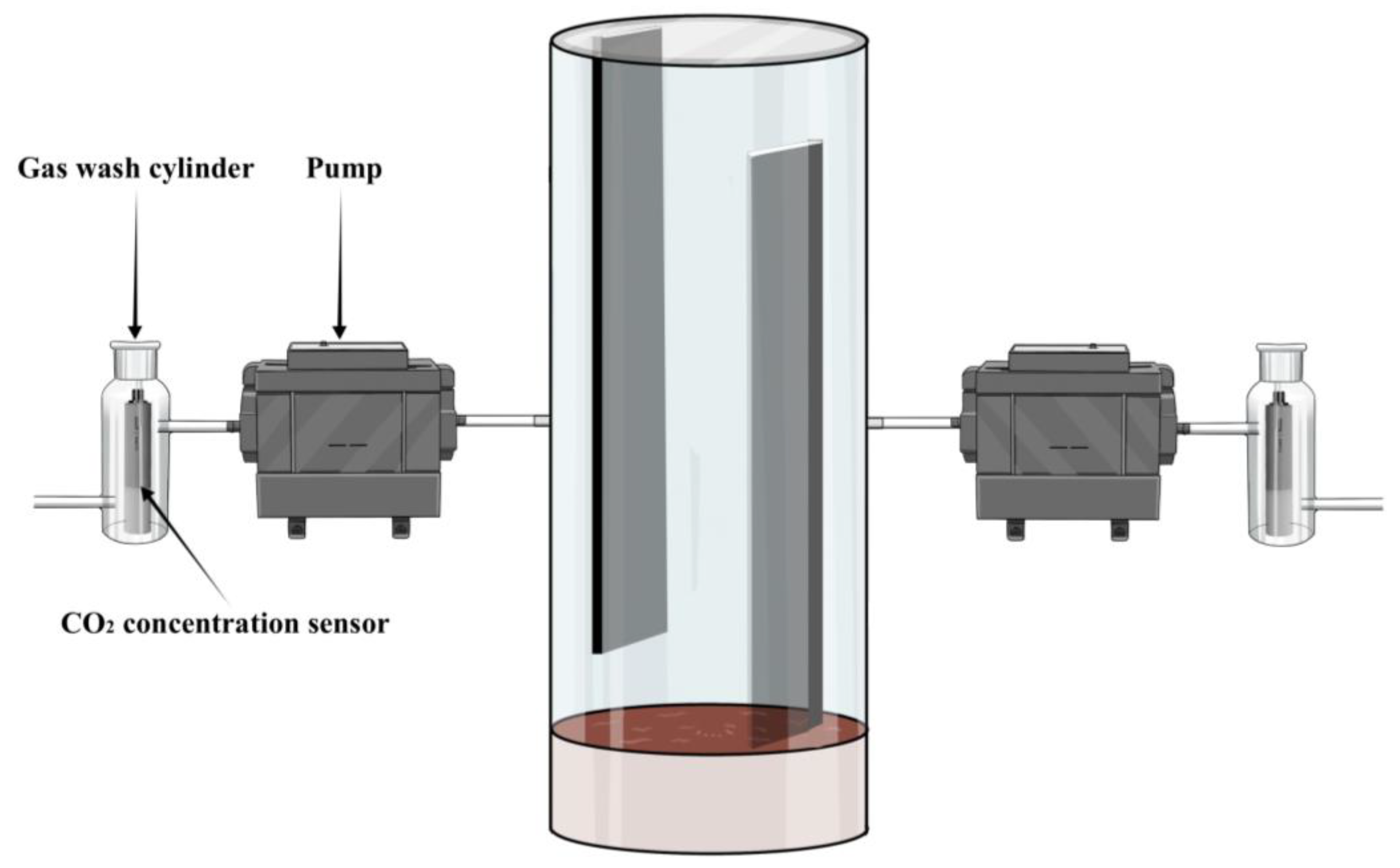
The measurement system consists of a chamber body, two carbon dioxide concentration sensors (Gmp252, Vaisala Oyj, Vantaa, Finland, accuracy: ±2% reading), two air pumps, two air hoses, and a soil collar. The chamber body consists of a transparent acrylic cylinder with a height of 1 m, a diameter of 0.3 m, and a thickness of 0.3 cm, with openings at both ends and a transparent acrylic chamber cover with a diameter of 0.32 m and a thickness of 0.3 cm, and favorable light transmission. The air chamber cover has an area of 0.071 m² and a volume of 0.071 m³. At the symmetrical ends of the column, an inlet pipe hole position and outlet pipe hole position are provided, with the inlet on the left side of the air chamber, 0.25 m away from the top cover, and the outlet hole on the right side of the air chamber, 0.25 m away from the bottom. To prevent the incoming airflow from directly colliding with the tested maize plant and generating a turbulent effect inside the air chamber, two deflectors are provided in the air chamber. The deflectors have a length of 85 cm, a width of 19 cm, and a thickness of 0.5 cm. The upper end of the deflector at the inlet is connected to the top cover, and the lower end is located 15 cm from the ground. The lower end of the deflector at the outlet is connected to the soil, while the upper end is located 15 cm from the top. The edges of the deflector and the inner wall of the air chamber achieve a close fit, and the maize crop is placed in the middle of the two deflectors. This design ensures that the airflow stemming from the air pump into the chamber first contacts the deflector and then smoothly enters the middle part of the chamber (between the two deflectors), limiting high turbulence in the middle of the deflector and the chamber wall. The soil collar is a ring-mounted, fluted, stainless-steel collar with a height of 8 cm, an outer diameter of 31 cm, and an inner diameter of 29 cm. The function of the collar is to prevent carbon dioxide gas from escaping through the gap between the bottom of the chamber and the soil, and the stainless-steel soil collars are buried below the tested crops several weeks in advance. Two carbon dioxide concentration sensors are placed in gas wash cylinders with 5 mm gas tube openings at the top and the tail. Figure 1 shows the basic structure of the instrument.

The gas wash cylinders, gas pumps, and body of the acrylic chamber are connected using a gas pipe (with an outer diameter of 6 mm and a thickness of 1 mm, made of plastic material) to form the intake module of the system; sequentially, the body of the chamber, the pump, and the gas wash cylinders with concentration sensors are connected using a gas pipe (with an outer diameter of 6 mm and a thickness of 1 mm) to form the pumping module of the system. Carbon dioxide concentration sensors are placed completely within the gas wash cylinders. The openings at the top and bottom of the gas wash cylinders ensure that the inflow of gas completely passes through the gas washing cylinder. The gas pump is connected to a gas flow meter (SMC PFM750, SMC Corporation, Tokyo, Japan) to adjust the needed flow rate during the experiment before the measurement, and the gas flow rates at the inlet and outlet are the same. Temperature and humidity sensors are installed inside and outside the chamber to monitor these environmental parameters during the field measurement.

2.3. Finite Element Modeling of the Air Chambers and Simulation Settings

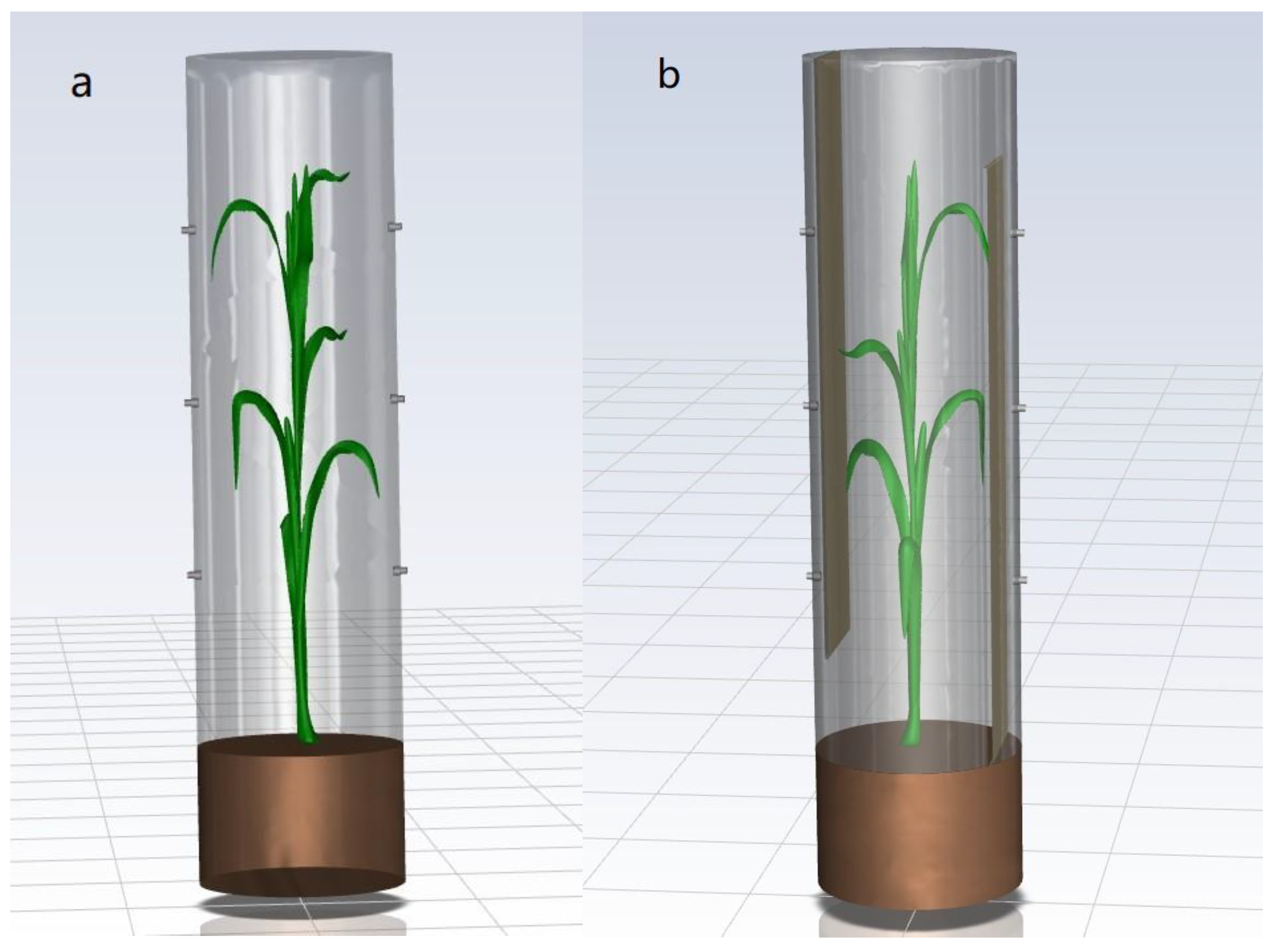
Finite element simulation modeling of the air chamber is conducted in Ansys Fluent 2020R2 software (ANSYS, Inc., Canonsburg, PA, USA). The model is established in a 1:1 ratio with the chamber sample, as shown in Figure 2. To reproduce gas diffusion, turbulence intensity, and concentration distribution conditions in the chamber as closely as possible, we add a finite element simulation model of a maize plant in the chamber. Due to the incorporation of the maize plant model, an unstructured mesh is implemented in this model. The number of meshes before adding the deflector is approximately 5 million, the minimum orthogonal quality is 2.40669 × 10⁻², the number of meshes after adding the deflector is approximately 6 million, and the minimum orthogonal quality is 3.06123 × 10⁻². The minimum orthogonal quality of the model mesh is closely correlated with the convergence and accuracy of the simulation results. Moreover, the minimum orthogonal quality of the worst cell is close to 0, while that of the best cell is close to 1, which indicates that our model mesh is accurate and that the simulation calculations converge more easily. The chamber bottom in the model is a porous medium with a height of 30 cm (this part of the height is calculated outside the chamber) to simulate gas emission from the surface of the agricultural soil. Figure 2 shows the two types of chamber models established in the Fluent 2020R2 software.

Although the morphology of each maize plant is unique, by including a maize model with a representative shape in the simulation, we can qualitatively analyze the gas concentration distribution and the turbulence state in the chamber, providing us with a basic reference framework.

The chamber without a deflector before modification and the modified chamber are simulated simultaneously. In the simulation experiments, the gas mass flow rates at the inlet and outlet of the chamber are set to 30 and 15 L/min, respectively, to investigate the time needed to reach the steady state and the turbulence effect generated in the chamber. The molar fraction of carbon dioxide in the initial state inside the chamber and gas introduced into the chamber through the air inlet is set to 0.0004 (400 ppm), the molar fraction of oxygen is set to 0.21, and the other gas composition parameters are maintained as default values. This is essentially the same as the gas concentration in the field measurement environment.

To simulate the nocturnal CO₂ emission resulting from maize leaf respiration, the maize leaves were defined as walls with a CO₂ molar fraction of 0.0008 (800 ppm). The CO₂ concentration on the surface of the leaf in the actual environment was estimated by evaluating the CO₂ concentration in the leaf cavity or the data of gas exchange within the leaf, and the CO₂ concentration within the leaf cavity tends to be lower than in the atmosphere because the leaf stomata form a diffusion barrier between the atmospheric CO₂ gas and the CO₂ in the leaf cavity. However, in the simulation experiment, gases diffuse from high to low concentrations, hence we set a higher CO₂ concentration at the leaf wall than the ambient CO₂ concentration. Daytime gas exchange across plant leaf surfaces, encompassing both respiratory CO₂ release and photosynthetic CO₂ uptake, is intricate. Our simulation setup is not designed to capture this complexity in full detail. We primarily focus on verifying the gas turbulence effect inside the chamber; hence, we exclusively simulate nighttime conditions, omitting plant photosynthesis. The bottom of the chamber features a porous medium to represent CO₂ emissions resulting from soil respiration. The emission rate is set to 4 μmol m⁻² s⁻¹, with the porous medium comprising 10 source terms.

The turbulence model in the simulation process is defined as the transition SST model. In some studies, the k-ε and k-ω models have been applied to investigate soil respiration within a small air chamber and gas exchange within a greenhouse, demonstrating a high degree of consistency with the real situation [14,30]. The k-ε model is very robust, but the results are significantly poorer in the presence of pressure gradients, separation, and considerable flow bends, which is suitable for the initial and parameterization calculations; the k-ω model is more suitable for capturing the boundary layer, free shear flow, and low-Reynolds number motion than the k-ε model, but the boundary is more sensitive, and the prediction of separation is less conservative [31]. The transition SST model combines the k-ε model under free flow conditions and the k-ω model near the wall, thereby using the k-ω model at the near wall and the k-ε model in the far field. In this study, due to the presence of the maize model, there is a large wall area inside the chamber and a boundary layer exists between the fluid and the wall. The transition SST model is more suitable for this simulation study, and more details on the transition SST model are provided below.

To ensure simulation accuracy, the simulation time step is set to 0.1 s and the number of iterations at each step is 10, based on our experience. A larger time step and iteration number could yield the same results as our settings, but this will greatly increase the computation time. The number of time steps for each simulation is 4200, lasting 6 min. Statistically, most chamber simulations reach a steady state within this time, and longer simulation times are not necessary.

2.4. Turbulence Model

Turbulence entails highly nonlinear and complex flow that can be simulated by certain numerical methods. The existing numerical simulation methods for turbulence can be divided into two categories: direct numerical simulation methods (DNS) and indirect numerical simulation methods [32]. Since the direct numerical simulation method does not need any assumptions or simplifications for turbulent flow, the performance requirements of the computational nodes are extremely high. Among the indirect numerical simulation methods, we selected the Reynolds averaging simulation method based on our specific circumstances.

The Reynolds averaging method is based on the derivation of the transient Navier–Stokes (N–S) equation. Although the transient N–S equation can be used to describe turbulence, its nonlinearity makes it extremely difficult to accurately depict turbulence details using analytical methods, and even if these details can be obtained, they are not very meaningful in engineering. The Reynolds-averaged Navier–Stokes (RANS) method, however, solves the homogenized N–S equations and represents the transient pulsation quantities by a certain model in time-averaged equations. The core of the RANS method is to solve the time-averaged N–S equations instead of directly solving the transient N–S equations. The RANS model aims to decompose all transient variables into their time-averaged components to derive time-averaged continuity and momentum equations, as expressed in Equations (3) and (4), respectively [33]:

$$\frac{\partial \rho }{\partial t}+\frac{\partial }{\partial x_i}\left(\rho {\mu }_i\right)=0$$

(3)

$$\frac{\partial }{\partial t}\left(\rho u_i\right)+\frac{\partial }{\partial x_i}\left(\rho u_i{u}_j\right)=\frac{\partial \rho }{\partial x_i}+\frac{\partial }{\partial x_j}\left[\mu \left(\frac{\partial u_i}{\partial x_j}+\frac{\partial u_j}{\partial x_j}-\frac{2}{3}{\delta }_{ij}\frac{\partial u_i}{\partial x_j}\right)\right]+\frac{\partial }{\partial x_j}\left(-\rho \stackrel{\overline{ }}{u_l^{\mathrm{’}}{u}_j^{\mathrm{’}}}\right)$$

(4)

In Equation (3), where $\rho$ denotes the fluid density, $t$ denotes time, $x_i$ is the $i$ component of the fluid velocity at a point in space, and ${\mu }_i$ is the $i$-th component of the velocity vector, representing the velocity of the fluid in the direction of $x_i$. In Equation (4), ${\mu }_i$ and $u_j$ are the $i$-th and $j$-th components of the velocity vector, respectively, μ denotes the dynamic viscosity of the fluid, and ${\delta }_{ij}$ denotes the Kronecker delta function, which is 1 when $i$ = $j$ and 0 otherwise.

The transition SST model used in this study is a turbulence simulation model based on the Reynolds-averaged Navier–Stokes equations.

The transition SST model is based on the coupling of the SST k-ω transport equations with two other transport equations. The SST k-ω model is a variant of the standard k-ω model, which is an empirical model based on modeled transport equations for the turbulent kinetic energy, k, and a specific dissipation rate, ω. As the k-ω model has been modified over the years, production terms have been added to both the k and ω equations, thereby improving the model’s accuracy in predicting free shear flows [34].

2.5. Verification of Instrument Precision

To validate instrument measurement accuracy, the alkali solution absorption method (A-A method) served as a baseline for comparison with the results obtained during the flow-through chamber measurements prior to initiating formal field data collection. To simulate the absorption of carbon dioxide by maize respiration, three 50 mL wide-mouth bottles, each containing 20 mL of a 1 mol/L NaOH solution, were placed at four points of equal height in the center of the gas chamber without a deflector plate and the flux in the chamber was continuously measured for one hour using the flow-through chamber method, during which the alkali solution reacted as follows:

2NaOH + CO₂→Na₂CO₃ + H₂O

(5)

Na₂CO₃ + CO₂ + H₂O→2NaHCO₃

(6)

The NaOH solution in the wide-mouth bottle continuously reacted with the carbon dioxide in the gas chamber, ultimately yielding NaHCO₃ in the solution. The residual NaOH was quantified via titrimetric analysis, employing a 1 mol/L HCl solution. The titration endpoint was indicated by a colorimetric change in phenolphthalein. This process is part of the methodology to measure the carbon dioxide flux in the gas chamber, which can be calculated by the alkali absorption technique as expressed in Equation (7):

$$F=\frac{\left(V_1-V_2\right)\cdot N}{T\cdot S}$$

(7)

In Equation (7), V₁ is the total volume of the NaOH solution distributed among the three wide-mouth bottles, V₂ denotes the volume of acid needed to titrate the remaining NaOH solution, N is the molarity of the HCl solution, S is the surface area of the chamber, and T denotes the experimental duration. The alkali solution in the gas chamber fulfills a twofold function: first, it functions as a proxy for carbon dioxide uptake via plant photosynthesis, thus modulating the carbon dioxide concentration in the chamber; second, it facilitates the precise determination of the gas flux in the chamber.

2.6. Field Measurement

In July 2023, we conducted in situ measurement experiments at the experimental site. We connected the gas intake and pumping modules to the air holes on both sides of the chamber using air tubes. Internal temperature and humidity sensors were placed at the center of the gas chamber, and external sensors were arranged on the top cover of the gas chamber. After the air pump was activated and the top cover of the chamber was closed, data was collected using a laptop computer by monitoring the readings of the carbon dioxide concentration sensors of the inlet and outlet modules. When the difference in the concentration between the two sensors remained at less than 5 ppm for more than 30 s, it was assumed that a steady state had been reached inside the chamber, and the top cover was opened to ventilate the chamber without shutting down the pump, thus accelerating the restoration of gas conditions in the chamber by continuously forcing gas outside the chamber into the interior. The air pump was not shut down to accelerate the restoration of environmental conditions inside the chamber by continuously forcing gas from the chamber to reduce the influence of the accumulated water vapor in the chamber on the subsequent measurements and to complete one measurement cycle.

For comparison, the same maize plant was measured on the second day in a chamber without a deflector, and the measurement procedure was the same as that described above.

3. Results and Discussion

3.1. Simulation Results

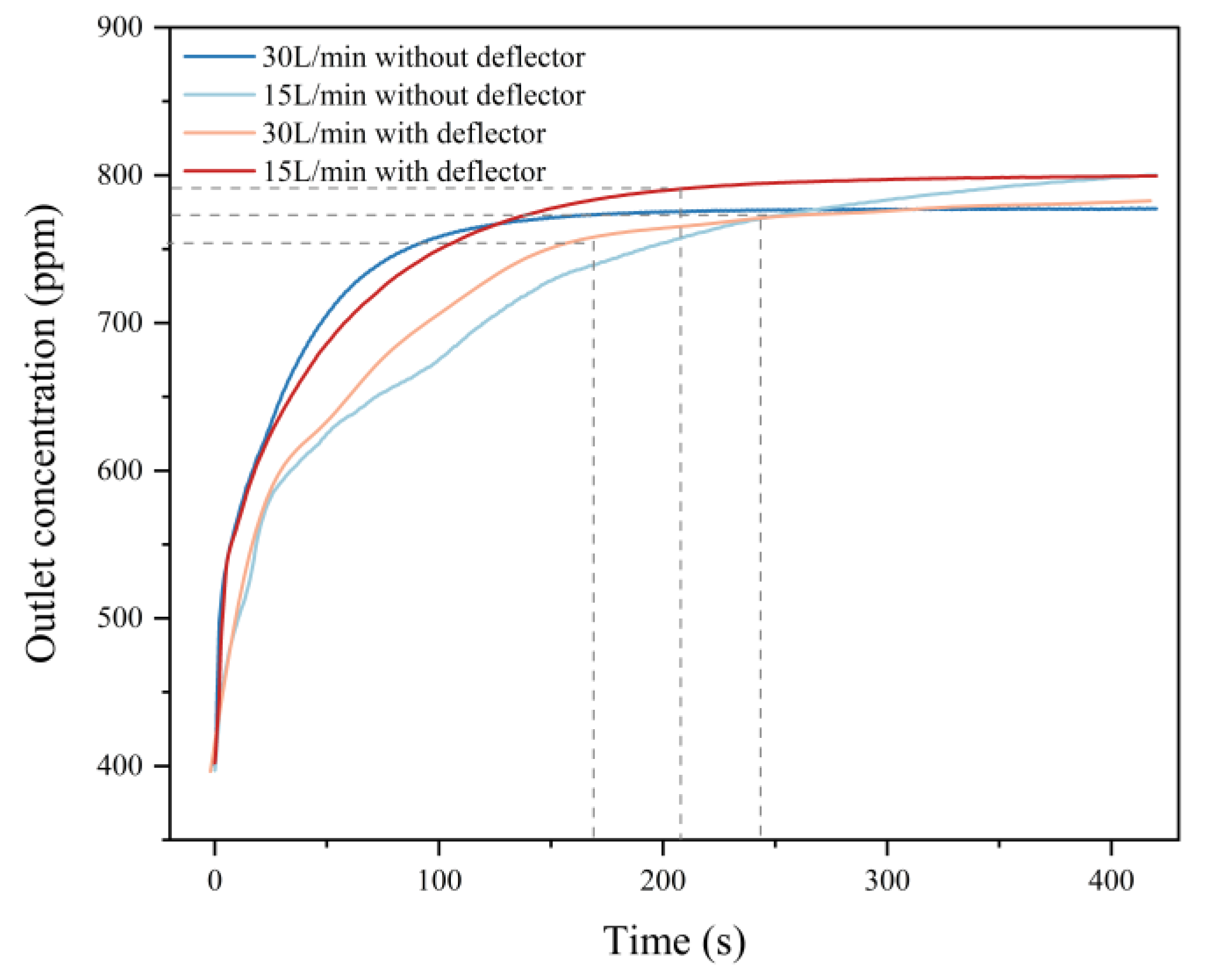
Before starting the simulation and based on real environmental conditions, we set the initial CO₂ concentration in the chamber to 400 ppm, the time step to 0.1 s, the maximum number of iterations to 10, and the simulation time to 420 s, which are sufficient to reach the steady state in most of the chamber. In our experience, the CO₂ concentration at the outlet remained stable in both the simulation and the on-site experiments. The concentration at the outlet of the chamber and the maximum Reynolds number of the effective measurement area within the chamber were monitored during the simulation. Simulations were performed with the unmodified and modified chambers using gas flow rates of 15 and 30 L/min. We set the chamber to reach a steady state when the variation in the CO₂ concentration at the outlet is less than 2%. The results are shown in Figure 3.

Three of the four simulation experiments reached a steady state within 420 s. The only exception was the simulation experiment with a low flow rate and no deflector. The simulation results showed that using a higher flow rate during measurements allows the chamber to reach the steady state faster, with or without the deflector; the addition of a deflector also reduced the time to reach the steady state at the same flow rate. With the addition of the deflector, the control group reached the steady state faster at the 15 L/min flow rate than the control group without a deflector at the 30 L/min flow rate. The simulation results showed that the addition of the deflector reduces the time required to reach the steady state in the flow-through chamber.

The state of the airflow in the air chamber can usually be quantified using the Reynolds number, which can be calculated using Equation (8) [35]:

$$Re=\frac{\rho \mathrm{V}L}{\mu }=\frac{\mathrm{V}L}{\nu }$$

(8)

In Equation (8), where $\rho$ (kg m⁻³) represents the density of the fluid, V (m s⁻¹) is the mean velocity of the fluid with respect to some object, L (m) denotes a characteristic linear dimension, $\mu$ (kg m⁻¹ s⁻¹) is the dynamic viscosity of the fluid, and $\nu$ (m² s⁻¹) is the kinematic viscosity of the fluid.

It is generally accepted that a Reynolds number Re < 2100 of the internal flow field indicates the laminar flow state, Re > 4000 indicates the turbulent flow state, and Re between 2100 and 4000 indicates the turbulent transitional flow state [36].

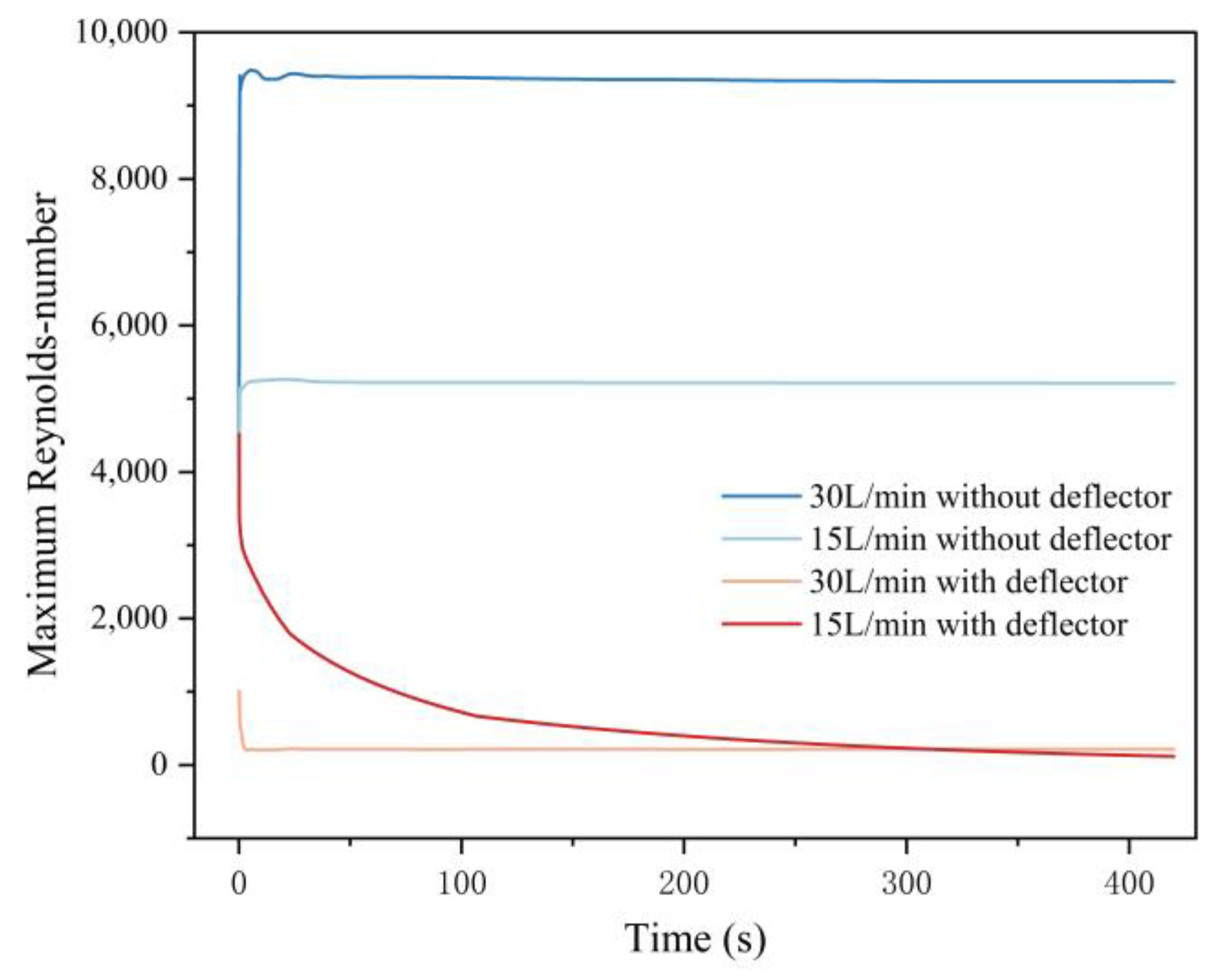
We also monitored the maximum Reynolds number inside the entire chamber during the simulation, and in the case of the simulation with the deflector, only the maximum Reynolds number in the effective measurement area between the two deflectors was monitored.

Figure 4 shows the maximum Reynolds number values inside the chamber for a seven-minute simulation. Without the deflector, the maximum Reynolds number reaches approximately 9330 at the gas flow rate of 30 L/min. Moreover, even at the lower gas flow rate of 15 L/min, the maximum Reynolds number reaches approximately 5214, which, according to the definition of the Reynolds number and turbulence, also indicates weak turbulence in the chamber. After adding the deflector, the maximum Reynolds number reaches approximately 215 at a gas flow rate of 30 L/min and approximately 151 at a gas flow rate of 15 L/min, suggesting that the airflow in the effective measurement area inside the chamber is completely laminar and no turbulence is generated. Since the number of leaves in the maize model used in our simulation is smaller than that of maize plants in the real measurement environment, the actual turbulence intensity in the chamber may be higher than that based on the simulation results.

According to the principle of the flow-through chamber, using a higher gas flow rate during the measurement can reach the steady state faster, and in earlier studies, it was suggested that the gas flow rate through the flow-through chamber should reach a value that enables complete gas exchange within the chamber every minute, and that lower flow rates cause the gas to remain in the chamber for too long, which is the main reason for the lower measured gas flux [37,38]. However, when using flow-through chambers to measure the carbon fluxes of taller plants (e.g., maize at the elongation stage in this study), the chambers are usually designed to be taller. In this case, continuing to use a gas flow rate that enables complete gas exchange within one minute in a chamber where only one plant is present will create a number of problems: (1) after the gas is directly forced into the gas chamber at a high flow rate, the direct collision with the leaves of the plant and the wall of the gas chamber may generate high turbulence in the gas chamber, which may lead to fluctuations in the gas distribution and the gas flow direction in the chamber and may impact the time needed to reach the steady state inside the chamber and the measurement results; this was verified in the subsequent simulation; (2) the gas produced by the gas pumps at high upper flow rates is relatively more unstable, and there may be a problem whereby the inlet and outlet flow rates are not completely consistent; hence, the flux calculation principle of the flow-through chamber cannot be applied and a pressure difference may be generated outside the chamber, which may result in the forced flow of carbon dioxide gas from the soil into the chamber interior, greatly reducing the accuracy of the measurement results.

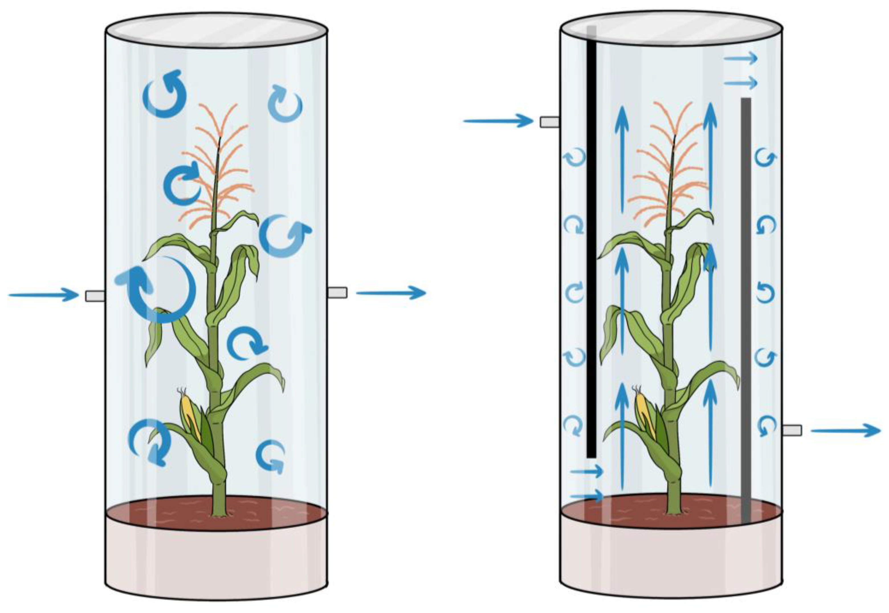
The unmodified chamber does not include a deflector, and air inlet and air extraction ports are arranged in the middle of the two ends of the chamber wall, which are directly connected to the air pump by air tubes for extraction and suction purposes. After the simulation of gas distribution and turbulence inside the chamber, it was found that because the gas is directly forced into the chamber from the air inlet (without an obstruction), high turbulence is generated due to the collision of the gas flow with the maize plant in the chamber. The dynamic behavior of the gas in the turbulent state increases the measurement complexity, and a longer time is needed to obtain stable measurement results, which could significantly impact the time needed to reach the steady state inside the chamber, the gas mixing conditions in the chamber, and the measurement results. In addition, the direct contact between the high-velocity gas flow and the chamber walls may cause an unwanted pressure increase in the chamber, possibly leading to gas leakage from the chamber [15]. The modified chamber structure with deflectors solves these problems.

The inclusion of a deflector forces the gas flowing into the chamber from the inlet to first collide with the deflector and then enter the chamber uniformly through the notch of the deflector at the bottom. The air pumps at both ends can force the gas in the chamber to flow according to the predetermined airflow route, and laminar gas flow is ensured within the effective measurement range of the chamber equipped with the deflector, after which the gas exits the chamber at the top through the notch at the outlet of the deflector. Figure 5 shows the gas state inside the gas chamber before and after the modification. The simulation results show that the addition of the deflector effectively eliminates turbulence in the chamber so that the gas flow enters the chamber at a more constant flow rate, mixes more evenly with the gas already inside the chamber, and produces a steady state faster, which is also demonstrated in the following field measurements.

3.2. Verification of Instrument Precision Results

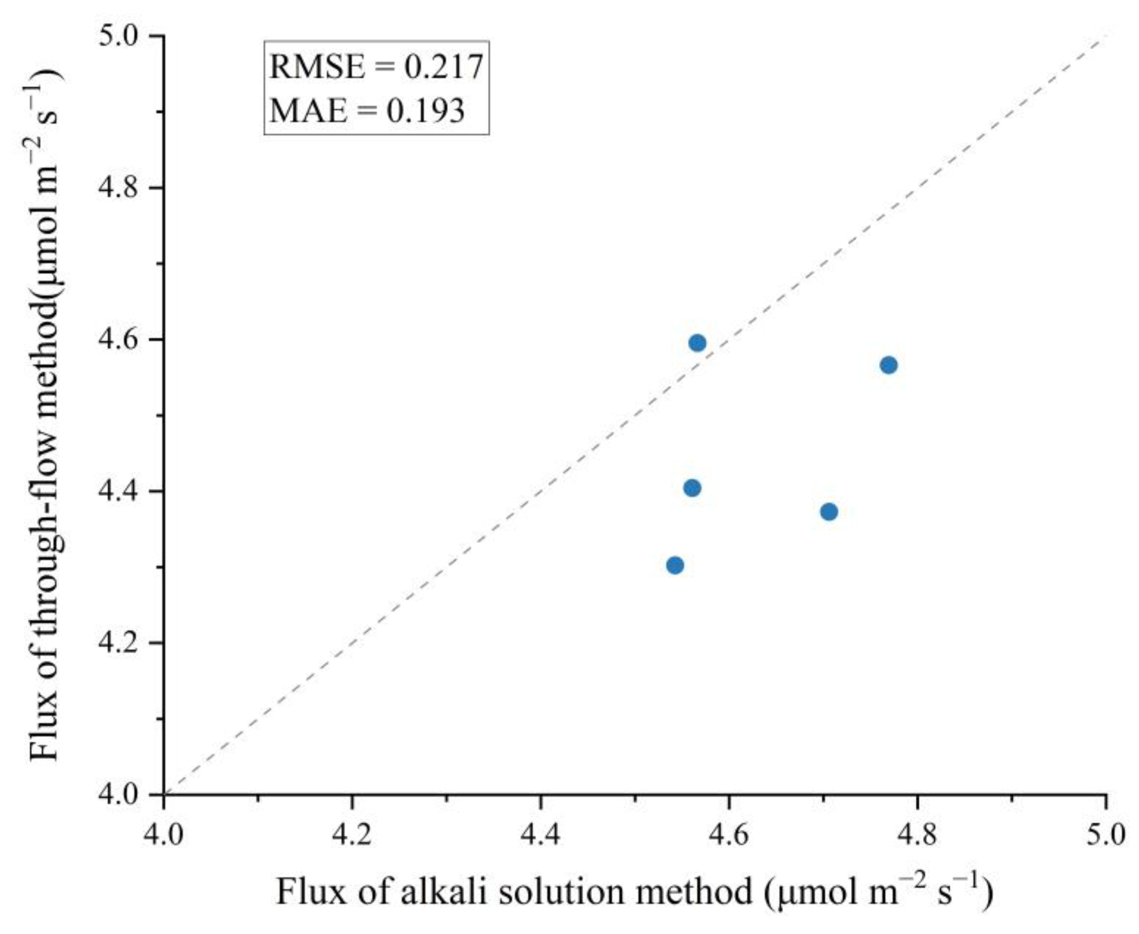
Results of the comparison of instrument precision verification using two methods are shown in Figure 6.

The analytical results revealed that the root mean square error (RMSE) between the flux values obtained by the alkali solution absorption method and the flow-through chamber approach is 0.217, while the mean absolute error (MAE) is 0.193. The observations indicated that in most instances, the flux values obtained using the alkali solution absorption method were slightly higher than those obtained using the flow-through chamber technique. This difference is likely attributable to the interaction between the carbon dioxide exhaled by the experimenter and the NaOH solution in the titration process, potentially leading to a deviation in the results. This result confirms the high precision of the instrument and the associated measurement technique utilized in our study.

3.3. Field Experiment Results

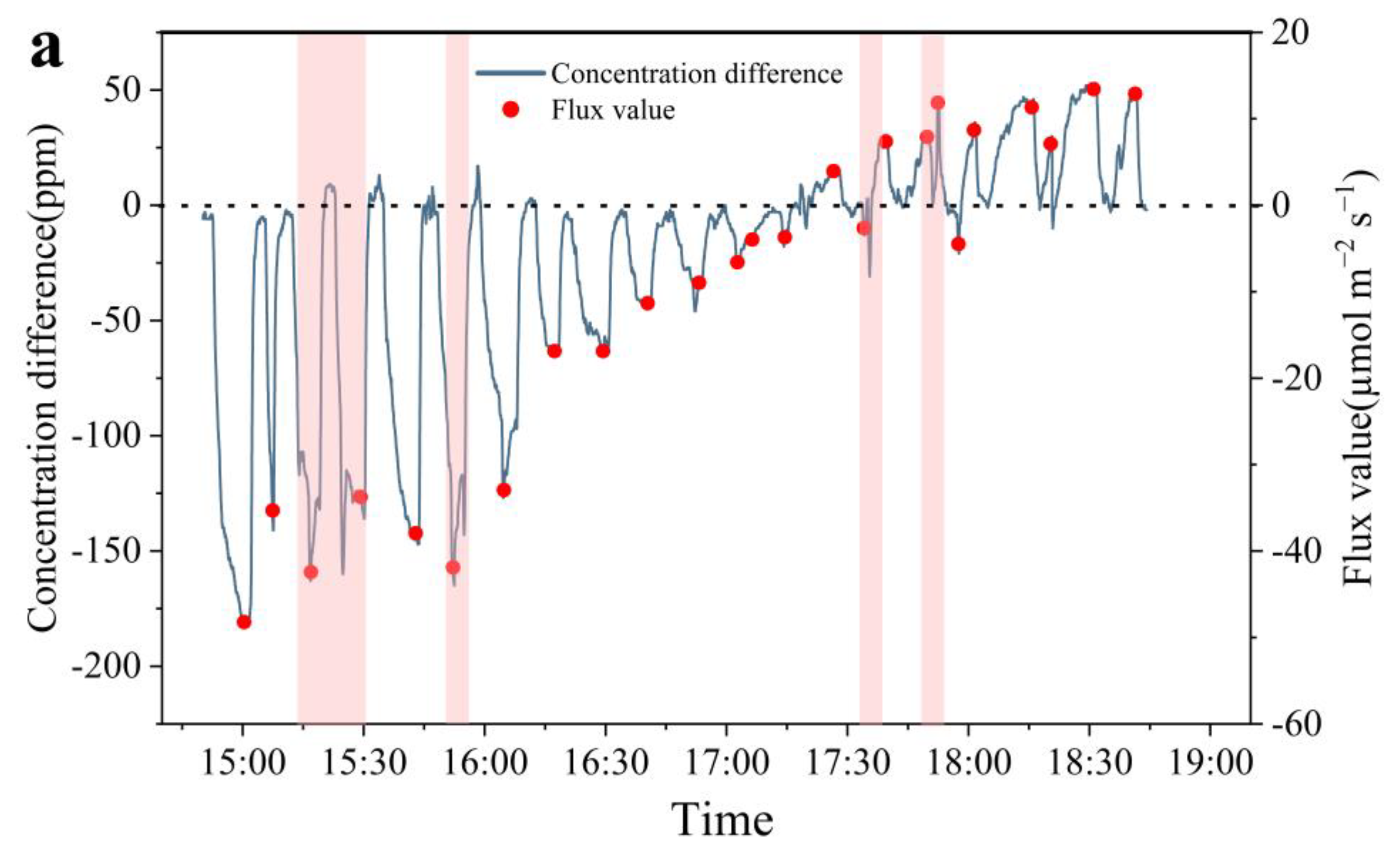
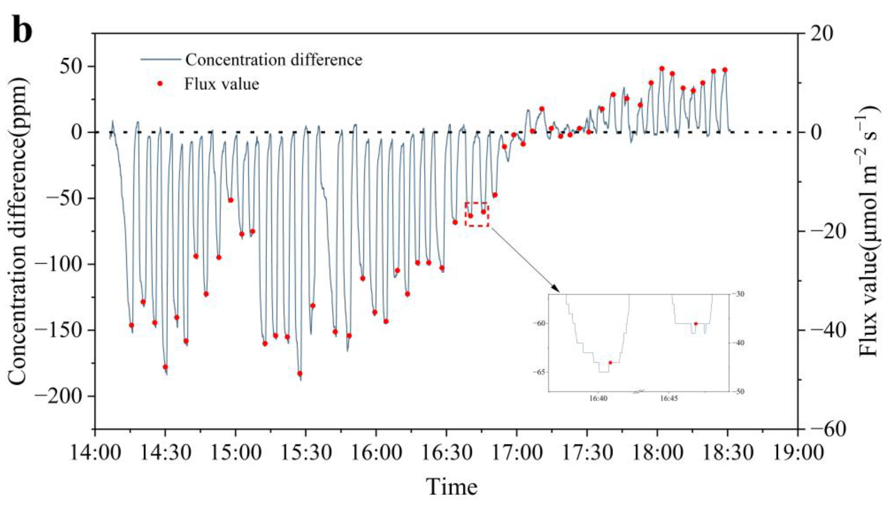
We conducted in situ measurements using both chambers from 2:00 p.m. to 7:00 p.m. on each of the two measurement days. The measurement results are shown in Figure 7. The flux result was calculated using Equation (2).

As shown in Figure 7, the blue curve is the difference between the outlet and inlet carbon dioxide concentration sensors. When the difference in concentration between the two sensors is smaller than 5 ppm for more than 30 s, it is considered that a steady state has been reached in the chamber, and the red dots indicate the flux values over one measurement period, which is calculated using the concentration difference when the steady state is reached using Equation (2). As shown in Figure 7, the net ecosystem flux showed a clear carbon sink-type trend in the afternoon, when the value of CO₂ absorbed by photosynthesis was greater than the CO₂ released by plant respiration, and the absorbed CO₂ flux fluctuated between 20 and 50 μmol m⁻² s⁻¹. At approximately 5:30 p.m., the amounts of carbon dioxide absorbed via photosynthesis and released via respiration were almost the same. At this time, the inlet and outlet concentrations of the two groups were basically the same, and the concentration difference fluctuated cyclically between −10 and 10 ppm, hence it was impossible to determine whether a steady state had been reached in the chamber based on the difference between the outlet and inlet concentrations. We timed the opening and closing of the chamber top during this period. In the absence of deflectors, the cover was operated at consistent intervals throughout the experiment duration, that is, once every 240 s in the group without a deflector and once every 120 s in the group with deflectors. This procedure was designed to prevent the build-up of external environmental variables such as temperature and humidity in the chamber, which could influence the measurement outcomes over extended closure periods. After 6 p.m., the ecosystem flux in the chamber transitioned into a carbon source. After sunset, and with the light intensity nearing zero, plant photosynthesis ceased. Consequently, the primary contributors to the ecosystem’s carbon dioxide flux were soil and plant respiration [39]. During this phase, the carbon dioxide flux observed in the chamber varied between 10 and 20 μmol m⁻² s⁻¹.

In the field measurement process, the average measurement period of the chamber system without a deflector was 561 s, while the average measurement period of the chamber system with the deflectors was 300 s. The addition of deflectors solved the turbulence problem in the chamber and altered the gas state in the measurement area of the chamber from turbulence to laminar flow, which reduced the measurement time by 46.5%, improved the measurement frequency, and decreased the change in the micrometeorological environment in the chamber during the measurement.

We found that the measured flux values were highly affected by light. During measurement of the experimental group with the deflectors, a half-hour period of cloudy weather occurred at approximately 3:00 p.m., which reduced the light intensity and affected plant photosynthesis, leading directly to a significant decrease in the measured flux values during this period, after which the flux returned to the previous level. In the measurement group without a deflector, it was cloudy from 4:00 p.m. to sunset, hence the measured flux values were also lower during this period.

Since environmental factors such as light and temperature always affect the carbon dioxide absorbed and emitted by photosynthesis and respiration [40,41], respectively, we could not conclude that the flux results of the modified chamber are more stable, but due to the elimination of turbulence in the chamber, the curves of the concentration difference for the modified chamber were more stable than those for the nonmodified chamber. Moreover, the curves for the modified chamber were less likely to show large variations in concentration differences, such as the pink area in Figure 7a, compared to those for the unmodified chamber. In the modified chamber, gas mixing exhibited enhanced homogeneity, thereby markedly reducing the occurrence of pronounced concentration gradients akin to those depicted in the pink region of Figure 7a. This improvement could increase the precision of the resulting flux measurements.

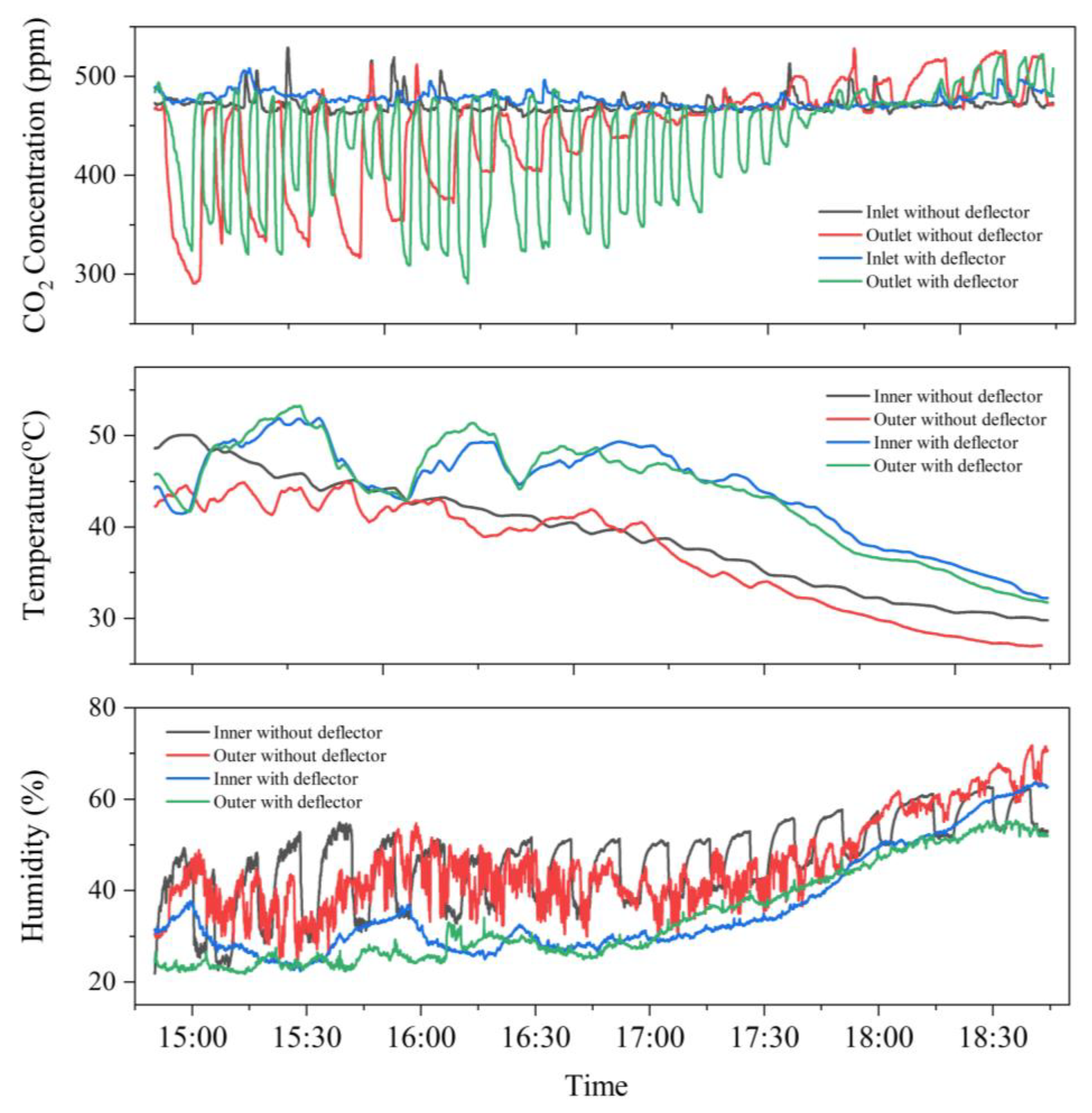
Figure 8 shows variations in the environmental factors during the measurement process. The ambient carbon dioxide concentration outside the chamber remained stable at approximately 480 ppm throughout the measurement. After the start of the measurement, the temperature and humidity in the two groups of chambers increased to different degrees after the top cover was closed. The average temperature difference between the inside and outside of the chamber without a deflector was 2.13 °C, and the average humidity difference was 11.50%. In contrast, the average temperature difference between the inside and outside of the chamber with deflectors was 1.01 °C, and the average humidity difference was 9.09%. Optimization of the chamber structure resulted in a 52.6% reduction in the mean temperature difference and a 20.1% reduction in the mean humidity difference. The reduced temperature and humidity differences observed during the measurement with the modified chamber could be primarily attributed to the increased frequency of the measurements. This higher frequency allowed for more frequent opening of the chamber top, thereby mitigating the fluctuations in the temperature and humidity. Throughout the intervals between the measurement periods, the air pumps remained operational and the chamber top cover was opened to closely align the internal chamber conditions with the external environmental factors. Significant variations in temperature and humidity could influence soil respiration and the physiological state of plants in the chamber [19]. These changes, in turn, could alter plant respiration and photosynthesis rates, subsequently impacting the precision of the measurements [42,43].

4. Conclusions

In this study, a flux chamber system based on the flow-through chamber method was developed and utilized to measure the net ecosystem carbon exchange fluxes of maize plants at the elongation stage. The experimental outcomes confirmed that the system could capture the net ecosystem carbon exchange flux of tall plants with both high frequency and precision.

To enhance instrument performance, we innovatively modeled both the gas chamber structure and the maize plant. Computational fluid dynamics simulations were conducted to analyze the gas conditions in the chamber, emphasizing the internal turbulence state. These simulations revealed that direct gas inflow into the chamber containing a tall plant could produce turbulence, prolonging the time needed to reach a steady state. This turbulence could further lead to significant temperature and humidity differences between the chamber interior and exterior during the measurements, thereby affecting the accuracy of the results.

The transition SST model in the CFD software Fluent 2020R2 was used to effectively simulate turbulence inside the chamber, especially considering the complex wall surfaces of maize blades. By simply adjusting the internal structure of the gas chamber, turbulent gas flow could be confined outside the core measurement zone. This ensured a homogeneous mixture of gases resulting from soil respiration, plant photosynthesis, and respiration in the central measurement area, facilitating faster and more consistent outflow.

Through both the simulation experiments and field measurements, it was confirmed that the modified chamber could achieve a more rapid steady state, offering enhanced measurement frequency and accuracy. The use of simulation technology facilitated comprehensive quantification of the regional gas states and preliminary evaluation of various gas chamber designs, setting the stage for actual measurements.

It is vital to note that turbulence in the flux chamber can often be overlooked in practical assessments. While turbulence is minimal in systems designed solely for soil respiration or those with smaller flux chambers due to the low flow rates and minimal plant interference, taller flux chambers designed for measurements of high crops inherently produce turbulence. Addressing this turbulence issue is essential for accurate gas flux measurements within these larger chambers.

This study, focusing on carbon flux measurements in maize, demonstrates the effectiveness of a flux chamber system that can be applied to various crops and ecosystems. Future research could utilize this system to understand crop-specific carbon dynamics under a range of environmental conditions, thereby improving data-driven carbon management in agroecosystems. Notably, this study reduced the impact of turbulence within the flux chamber; however, there is still potential for further refinement. Future studies might explore alternative designs of the chamber’s internal architecture to optimize gas homogenization and accelerate the attainment of equilibrium. Furthermore, given the significant impact of external temperature and humidity on data accuracy, subsequent efforts should concentrate on enhancing the environmental control mechanisms within the chamber. Such improvements are anticipated to markedly increase the precision and reliability of flux measurements.