Article

Improve the Simulation of Radiation Interception and Distribution of the Strip-Intercropping System by Considering the Geometric Light Transmission

1
State Key Laboratory of Water Resources Engineering and Management, Wuhan University, Wuhan 430072, China
2
Dongjiang River Basin Administration of Guangdong Province, Huizhou 516000, China
3
College of Agricultural Science and Engineering, Hohai University, Nanjing 210098, China
*
Authors to whom correspondence should be addressed.
Agronomy 2024, 14(1), 227; https://doi.org/10.3390/agronomy14010227
Submission received: 20 November 2023 / Revised: 26 December 2023 / Accepted: 9 January 2024 / Published: 22 January 2024
(This article belongs to the Section Innovative Cropping Systems)

Abstract

:
Intercropping radiation interception model is a promising tool for quantifying solar energy utilization in the intercropping system. However, few models have been proposed that can simulate intercropping radiation interception accurately and with simplicity. This study proposed a new statistical model (DRT model), which enables the simulation of daily radiation distribution by considering the geometric light transmission in the intercropping system. To evaluate model performance, the radiation interception and distribution in two wheat/maize strip intercropping experiments (A and B) were simulated with the DRT model and other two statistical models, including the horizontal homogeneous canopy model (HHC model) and the Gou Fang model (GF model). Experiment A was conducted in different intercropping configurations, while Experiment B was conducted in soils with different salinity levels. In both experiments, the HHC model exhibited the poorest performance (0.120 < RMSE < 0.172), while the DRT model obtained a higher simulation accuracy in the fraction of photosynthetically active radiation (PAR) interception, with RMSE lower by 0.008–0.022 and 0.022–0.125 than the GF and the HHC models, respectively. Especially, the DRT model showed stronger stability than the other two models under soil salinity stress, with R2 higher by 0.129–0.354 and RMSE lower by 0.011–0.094. Moreover, the DRT model demonstrated a relatively ideal simulation of the daily radiation distribution in Experiment A (0.840 < R2 < 0.893, 0.105 < RMSE < 0.140) and Experiment B (0.683 < R2 < 0.772, 0.111 < RMSE < 0.143), especially when the continuous canopy formed during the later crop growth stages. These results indicate the superiority of the DRT model and could improve our understanding of radiation utilization in the intercropping system.

1. Introduction

Intercropping, a productive practice of growing two or more crops simultaneously in the same field, has received more interest and is widely used across the world [1,2]. Due to the critical demand for mechanized agriculture, relay strip intercropping gets more attention and development [3]. For relay strip intercropping, adequate radiation interception of the crop aboveground is a primary advantage of intercropping, it affects the crop photosynthetic process and increases yields [2,4]. To enhance agronomic management and optimize yields in intercropping systems, it is essential to quantify the radiation transmission of the intercropping system accurately.
The radiation interception model is an effective tool for simulating radiation interception and partitioning of field crops in strip intercropping systems. Two types of models can be classified according to their modeling principles: the geometrical model and the statistical model [5]. The geometrical model considered instantaneous light transmission in the canopy and more details such as heterogeneous canopies [6], border row effects [7], and strip orientation [8]. Gijzen and Goudriaan [9] may first propose a geometrical model considering the direction of incident light and the canopy architecture. Subsequent studies applied the model in practice and improved its accuracy [10,11,12]. Munz, Graeff-Honninger, Lizaso, Chen, and Claupein [11] used the geometrical model to calculate the available radiation at the top of the subordinate crop canopy to describe the incoming light distribution of the subordinate crop. The geometrical model improves our understanding of the radiation transfer in the intercropping system and generally can obtain high simulation accuracy; however, the geometrical model is restricted in use due to its complexity [10,13]. Numerous input variables need to be measured in the geometrical model, such as row orientation, leaf area density, canopy extinction coefficient (gψ and kψ), plant height (H), and the exact corresponding time.
Different from the geometrical model, the statistical model simplifies plant canopies as homogeneous and turbid cuboids using the strip-crop approach [14]. Based on the hypothesis, the statistical model can estimate the daily radiation interception of crops with fewer variables, such as the horizontal homogeneous canopy model (HHC model), employed in the popular crop model APSIM, which has been widely used in radiation interception simulation. Pronk et al. [15] introduced the “view factor” and “compressed canopy” theories and proposed an empirical model based on Beer’s law to calculate the radiation interception by only four easily obtained input variables/parameters, including H, leaf area index (LAI), strip and path width (R and P), and extinction coefficient (k). Zhang, et al. [16] used this method to calculate light interception in wheat-cotton relay intercrops. Wang et al. [17] attempted to allocate the residual indirect light of the “view factor” theory to each individual crop of wheat/maize strip intercropping system. To further improve model accuracy, Gou et al. [18] separated the taller intercrop canopy into the upper layer (strip-planted sole crop) and the under layer (two crops with the same height), considering the penetrated light from the upper layer as the incident light of the under layer. Numerous studies have proven the effectiveness of Gou’s model (GF model) and applied it in strip intercropping simulations [2,19,20,21,22]. For example, Pinto, van Dam, van Lier, and Reichardt [22] chose the latest GF model to calculate the radiation interception of each crop in the newly proposed intercropping model. And Pierre et al. [23] also chose the GF model as the method of calculating radiation interception in DSSAT.
However, there are still several limitations regarding the statistical model. The accuracy of the simplified statistical models could be restricted [10]. The statistical model generally fails to capture spatial differences in instantaneous light transmission due to the simplification of the light angle in simulation [11]. Meanwhile, though the radiation interception of the whole canopy can be verified using existing statistical models, the radiation interception partitioning for each crop is difficult to quantify [13]. Explaining the light transmission in the canopy may be a persuasive method for the radiation interception partitioning of statistical models. To address these issues, we proposed a novel radiation interception model for the relay strip intercropping system, the DRT model, which considers the angles of light in a two-dimensional plane and calculates the temporal and spatial integration for both direct and indirect light. Other two statistical models, a horizontally homogenous model (HHC model) and a GF model, were selected to compare. To comprehensively assess the accuracy and stability of these models, this study utilized two sets of independent experimental data. The first experiment focused on the accuracy of the model under different intercropping configurations, while the second experiment targeted the model’s accuracy and stability under different soil salinity stresses. The objectives of this study were to (1) develop a new radiation interception model for relay strip intercropping, (2) test the model performances for simulating radiation interception in different intercropping experiments, and (3) propose a simplified approach to simulate daily light distribution and test its performances.

2. Materials and Methods

2.1. Model Theory

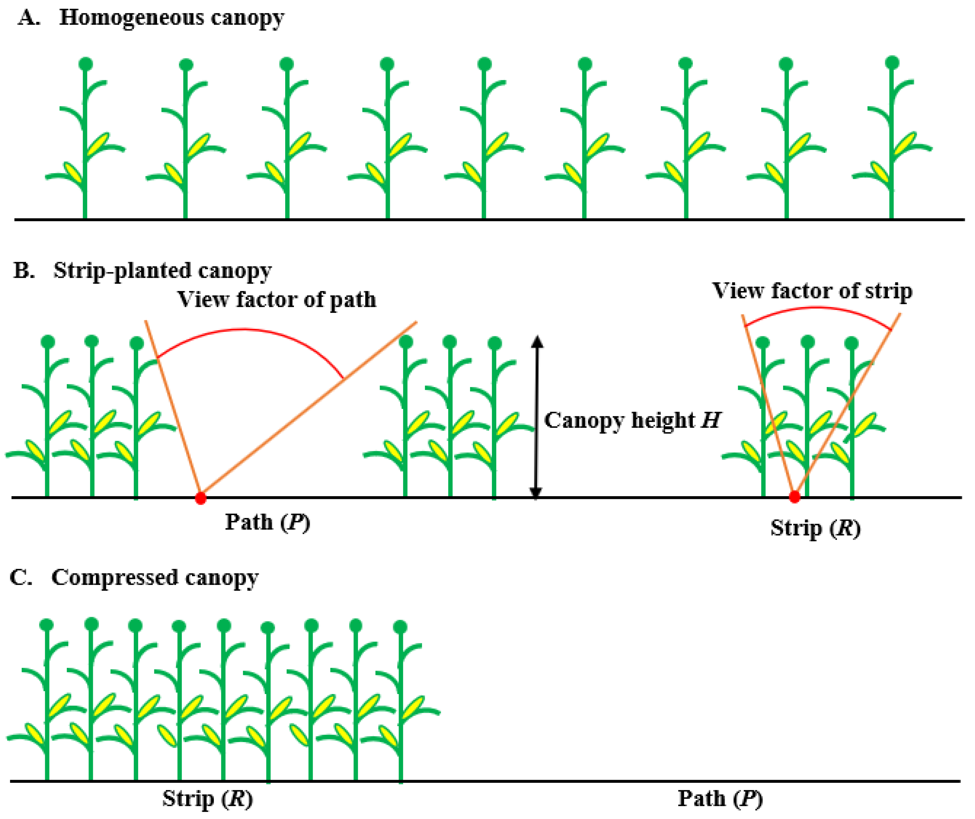
2.1.1. Horizontally Homogeneous Canopy Model (HHC Model)

Taking a two-crop intercropping system as an example, the whole canopy is divided into two horizontally homogeneous layers in the HHC model. The layer boundaries are at the top of the two crops’ canopy. The fraction of light transmitted out from the bottom of the upper layer is the fraction entering the lower layer. The upper layer contains only the taller crop, encompassing a fraction of its LAI. While the lower layer is a two-crop mixed canopy, comprising the remaining LAI of the taller crop and the LAI of the short crop, LAI is assumed to follow the power of five functions with the relative height as follows:
L A I ( h ) = h 5
where h is the relative height (0 at the bottom and 1 at the top of the canopy). In the lower mixed canopy, the fraction of radiation interception of each crop with the same height is calculated as Equations (2)–(4):
f intercropps = 1 e k 1 L A I 1 k 2 L A I 2
f intercropps _ 1 = k 1 L A I 1 k 1 L A I 1 + k 2 L A I 2 f intercropps
f intercropps _ 2 = k 2 L A I 2 k 1 L A I 1 + k 2 L A I 2 f intercropps
where fintercrop_1 and fintercrop_2 are the fractions of radiation interception of crop 1 and crop 2 in the mixed canopy, respectively; k1 and k2 are the light extinction coefficients of crop 1 and crop 2; LAI1 and LAI2 are the leaf area indexes of crop 1 and crop 2. The HHC model has been applied in the Canopy module of the APSIM (Version 7.9) [2]; more details can be found on the website (http://www.apsim.info, accessed on 3 May 2017) [24].

2.1.2. Gou Fang Model (GF Model)

Similar to the HHC model, the GF model divided the canopy into two layers according to the height difference between the two intercropping crops. The upper layer can be assumed to be a strip-planted canopy with a single crop with some rows omitted, which creates a compressed canopy and empty paths (Figure 1B). The fraction of light interception with the same LAI of a strip-planted canopy is numerically between the homogeneous canopy (as the maximum, Figure 1A) and the compressed canopy (as the minimum, Figure 1C). A weight (w) is used in the empirical function to calculate the fraction of light interception by a strip-plant canopy (fstrip) as follows:
f strip = f homo × 1 w + f compr × w
The fraction of light interception in the homogeneous canopy (fhomo) and compressed canopy (fcompr) are both calculated by Beer’s Law. For the compressed canopy, the LAI in the green part of the field can be converted to a compressed LAI by strip width (R) and path width (P):
f homo = 1 e k × L A I
f compr = 1 e k × L A I compr × R R + P
L A I compr = L A I × R + P R
where k is the light extinction coefficient.
The value of w is between 0 and 1, and can be calculated as follows:
w = S P S R 1 e k × L A I compr
where SP and SR are the fractions of light transmitted to the soil surface in the path and under the strip, respectively. The larger w means more light is transmitted to the soil surface in the path than that in the strip, indicating that the strip-plant canopy is closer to a compressed canopy. On the contrary, a smaller w indicates the strip-plant canopy is closer to a homogeneous canopy. SP and SR can be calculated as follows:
S P = I P black + 1 I P black × e k × L A I
I P black = H 2 + P 2 H P
S R = I R black × e k × L A I compr + 1 I R black × e k × L A I
I R black = H 2 + R 2 H R
Equations (11) and (13) are obtained by spatial (from 0 to P/R, respectively) and angular (from θ to π/2) integration. The detailed integration process was shown in Pronk, Goudriaan, Stilma, and Challa [15]. From Equations (10) and (12), we can know SP and SR are coming from two origins. For radiation transmitted to the soil surface of the path (SP), one is direct radiation, which depends on the view factor over the path (IPblack), and the other is transmitted from neighboring one or several crop rows (1 − IPblack). The precise calculation of transmitted radiation (1 − IPblack) is supposed to be a spatial (from 0 to P/R) and angular (from 0 to θ) integration integrated like direct radiation. The integrand is the radiation that falls on the soil surface after being intercepted by a certain thickness of compressed canopy, which is determined by the geometric relationship. The remaining radiation from the upper canopy interception along the path serves as the incoming light for the compressed canopy of the shorter crop, while the remaining radiation from the strip acts as the incoming light for the compressed canopy of the taller crop with a part of its LAI.

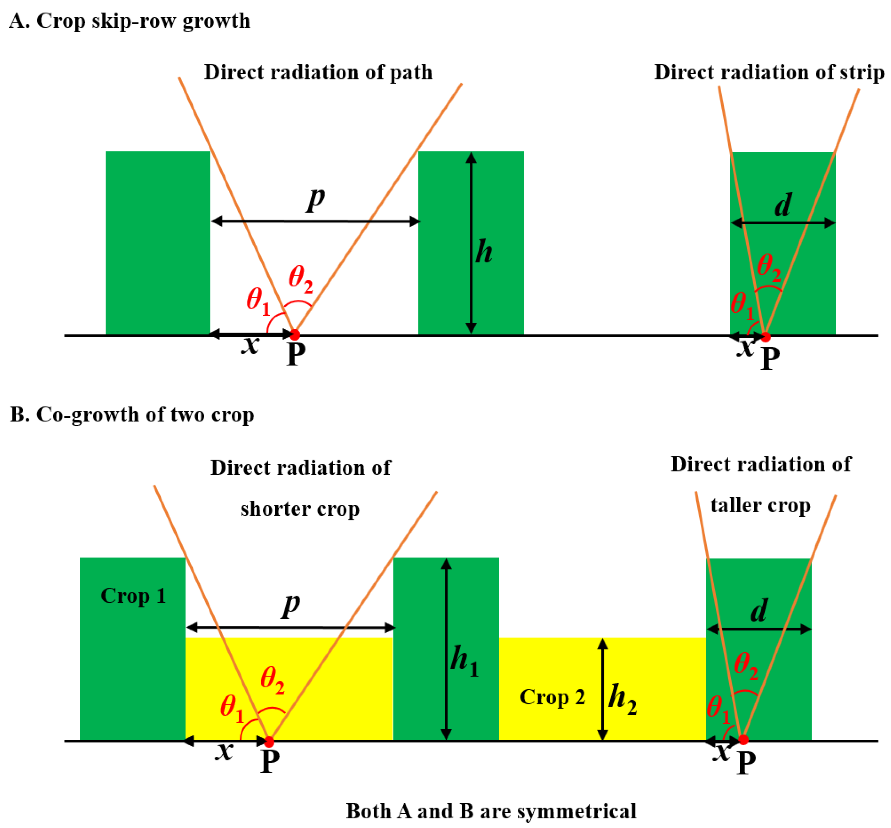
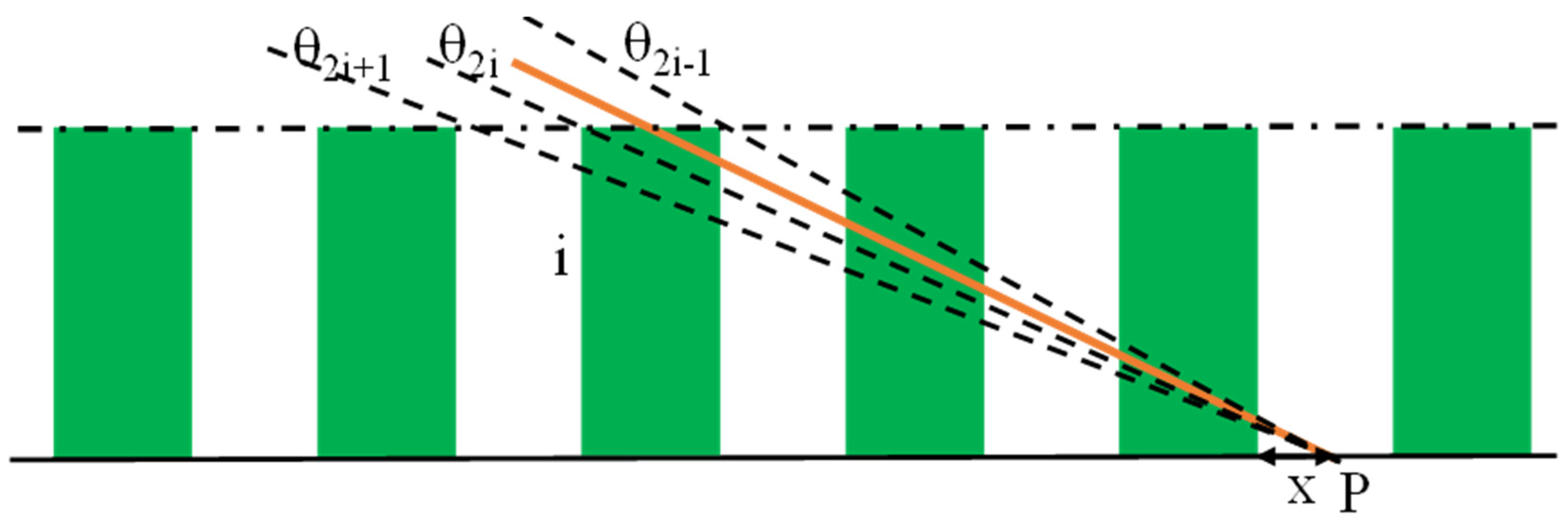
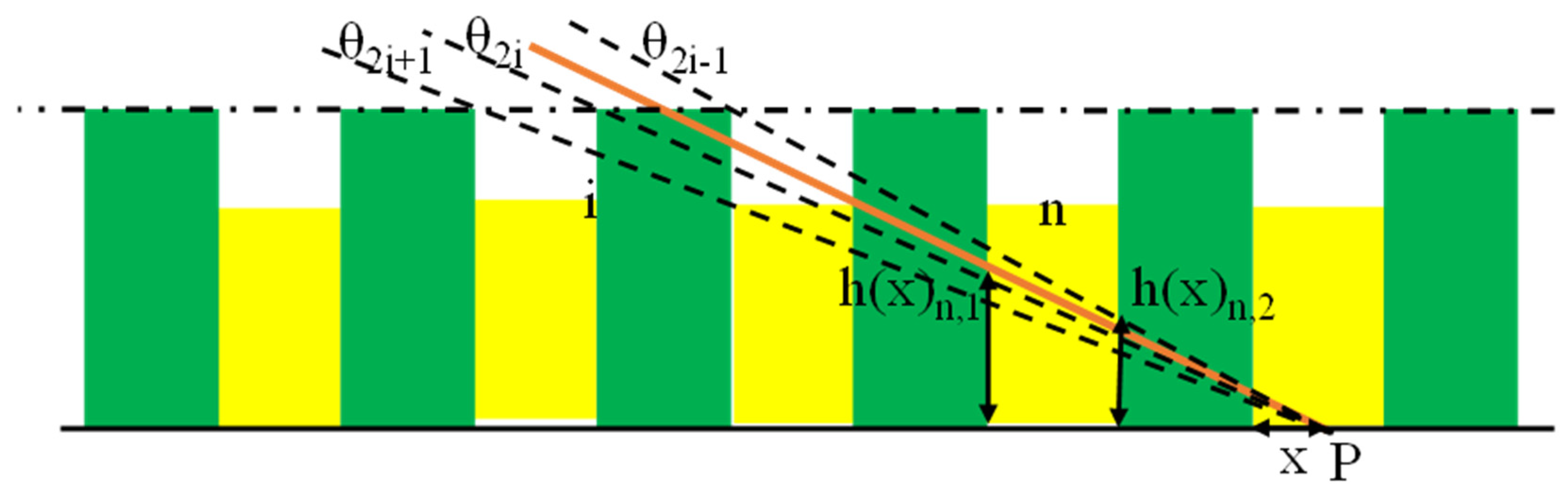
2.1.3. Daily Radiation Transmission Model (DRT Model)

We developed a statistical daily radiation transmission model (DRT model), referring to the quantifications of instantaneous radiation transmission in the geometrical model. The DRT model comprises three modules: crop skip-row growth, co-growth of two crops, and spatial distribution of daily radiation transmission.
Module 1: Crop skip-row growth
For the crop skip-row growth (Figure 2A), the radiation interception of the single crop (f), for example, an intercropping unit (strip and path, d + p), is the total radiation minus the radiation reaching the soil surface as follows:
f = 1 I p , d + I p , i I d , d + I d , i
where Ip,d and Id,d are the direct radiation on the path and the strip; Ip,i and Id,i are the indirect radiation (through the canopy) on the path and strip, respectively. These variables can be calculated based on view factor theory and radiation geometry principles. The detailed calculation equations for these variables are in Appendix A.
Module 2: Co-growth of two crops
In the co-growth of two crop situations (Figure 2B), the radiation interception of crop 1 and crop 2 (F1 and F2) corresponds to the summation of their respective direct and indirect radiation components along strip d and strip p:
F 1 = F 1 d , d + F 1 p , i + F 1 d , i
F 2 = F 2 p , d + F 2 p , i + F 2 d , i
where F1d,d and F1d,I are the radiation interception of direct and indirect light along strip d of crop 1, respectively; F1p,i is the radiation interception of indirect light along strip p of crop 1; F2p,d and F2p,i are the radiation interception of direct and indirect light along strip p of crop 2, respectively; F2d,i is the radiation interception of indirect light along strip d of crop 2. The calculation of these variables is shown in Appendix B.
Module 3: Spatial distribution of daily radiation transmission
The spatial daily light interception can be calculated in the DRT model, it is a function of the geometrical models but not available in other statistical models. It has two steps. First, due to the position of simulated points (x) being controlled by the position of Gaussian points (an), it is necessary to ensure the alignment between the positions of the Gaussian points and the measured PAR points. The method for selecting Gaussian points is in Appendix C. Secondly, unlike calculating the total direct radiation interception on the strip, it is necessary to calculate the light interception of the direct radiation at every Gaussian point. The calculation of the indirect radiation (rp(x) and rd(x)) in Module 3 is identical to Module 1 and Module 2. The angle of integration of direct radiation at the Gaussian point is calculated as follows:
The crop skip-row growth:
I p , x = r p ( x ) + θ 1 , x π 2 sin θ d θ 0 π 2 sin θ d θ = r p ( x ) + cos θ 1 , x = r p ( x ) + x x 2 + h 2
I d , x = r d ( x ) + x x 2 + h 2 · e k · L A I c
Co-growth of two crops:
I p , x = r p ( x ) + x x 2 + h 2 · e k 2 · L A I 2 , c
I d , x = r d ( x ) + x x 2 + h 2 · e k 1 · L A I 1 , c
where x represents the position of that Gaussian point; x = an × d when calculating Id,x; x = an × p when calculating Ip,x. Ip,x is the fraction of radiation that falls on the x point along the strip of the shorter crop (p); Id,x is the fraction of radiation that falls on the x point along the strip of the taller crop (d).
The angle integration in Module 3 is from 0 to π/2, while the daily radiation is from 0 to π. Therefore, the results need to be converted into daily radiation interception. Due to the geometric symmetry in the DRT model, the radiation interception at the points exhibits horizontal symmetry as well. The symmetric points need to be averaged to represent the radiation interception at the two points.

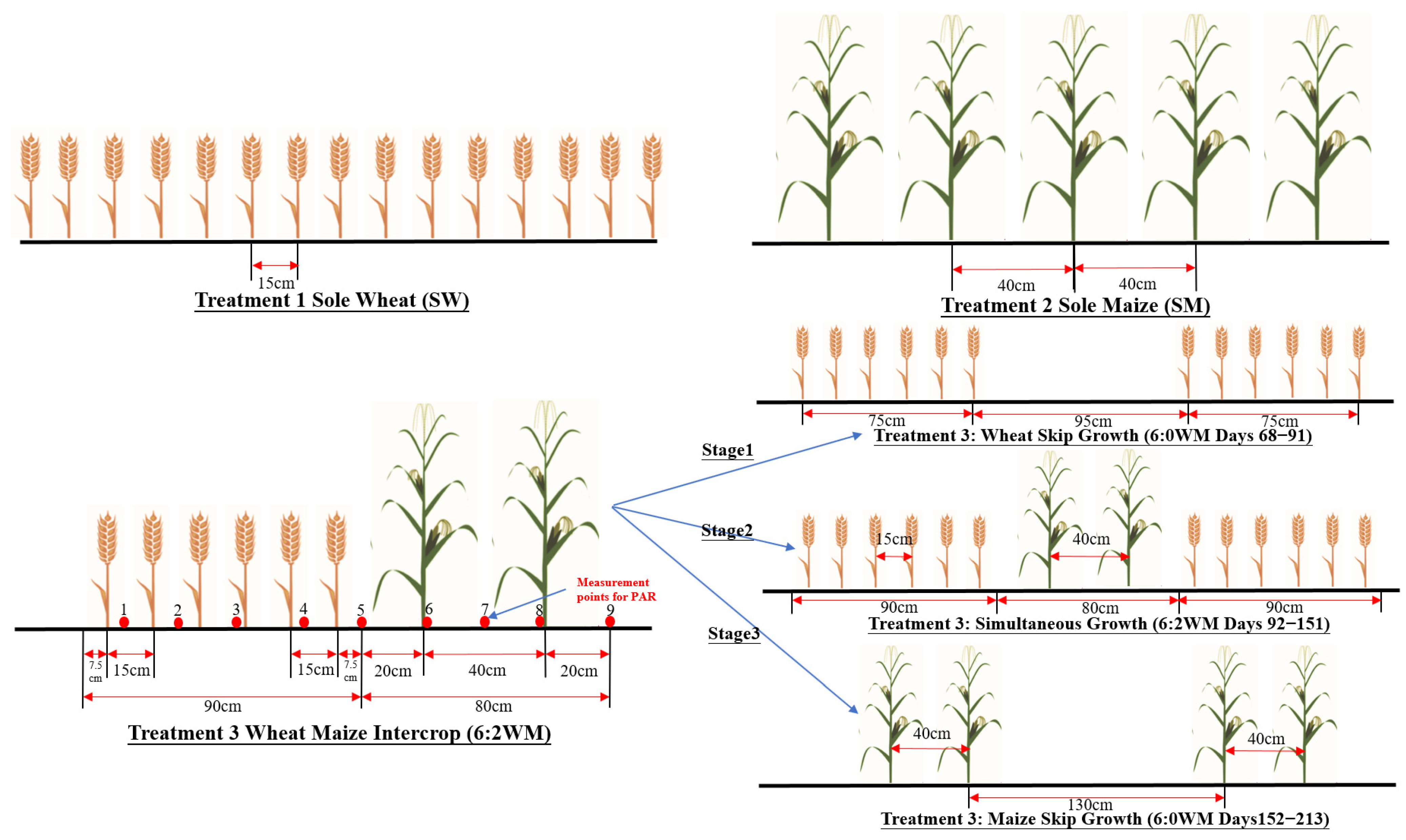
2.2. Experimental Data Collection

In this study, two wheat-maize intercropping experiments A and B were selected to evaluate the model performances. Experiment A was conducted in the Wageningen field experiment (51°59′20″ N, 5°39′16″ E). Five wheat-maize intercropping configurations were designed in Experiment A, including 6:0 WM (wheat skip growth), 0:2 WM (maize skip-row growth), 6:2 WM, 6:3 WM, and 8:2 WM (three different treatments of co-growth of wheat and maize). The details of Experiment A can be found in Gou et al. [18].
Experiment B was conducted in an experimental station at Wuhan University, Hubei Province, China (30°32′36″ N, 114°22′09″ E). Two sole crop systems of wheat (Treatment 1) and maize (Treatment 2) and a wheat-maize intercropping system (Treatment 3, the intercropping ratio is 6:2 WM) were designed (Figure 3). Moreover, the crops in each treatment were planted in fields with three soil salinity levels (S1, S2, and S3). Specifically, the average electrical conductivity of the saturation extract (ECe) values in the three fields were 0.89–1.18, 1.98–2.96, and 2.63–6.42 dS m−1 in S1, S2, and S3, respectively. The row spaces of each treatment are shown in Figure 3. The wheat variety is Zhengmai9032, and the maize variety is Hunong101. The row orientation was north-south direction. Winter wheat was sown on 20 November 2022, and harvested on 31 May 2023. Maize was sown on 15 March 2023, and harvested on 1 August 2023. Before wheat sowing, a compound fertilizer of N-P2O5-K2O is applied, and the application rates of nitrogen, phosphorus, and potassium were 180 kg ha−1, 75 kg ha−1, and 100 kg ha−1, respectively.
In Experiment B, the leaf area and height of two crops in each field were determined by the average status of three independent measurements. The leaf areas of the maize and wheat were calculated based on LA = 0.75 × L × W and LA = 0.85 × L × W (L and W are the length and width of the measured leaf), respectively. The plant height is defined as the distance from the soil surface to the top of the canopy. The crop height measurement was conducted on the same day, with LAI measurements about once every two weeks from crop emergence to the final harvest. During the crop growth period, we measured light interception 12 times. Each measurement involved three separate recordings within one day, conducted at 10:00 a.m., 12:00 p.m., and 2:00 p.m. The daily light interception at each measurement point was determined by the average of three recordings. Photosynthetically active radiation (PAR) above and below the canopy (about 5 cm above the soil surface) was measured using a Beam Fraction Sensor (BFS, a quantum sensor). Five values were collected during each measurement. The SunScan probe was parallel to the rows at the measured points. Four different points were measured in Treatments 1 and 2, and nine different points were measured in Treatment 3 and its different growth stages (Figure 3). In Treatments 1 and 2, measurements were used to calibrate the k of wheat and maize. In Treatment 3, measurements were made at approximately 19 cm intervals across a width of 170 cm. The overall fraction of light interception in the heterogeneous canopy was calculated as the arithmetic average of measurements at the nine different measured points.

2.3. Statistical Indicators

In this study, R-square (R2) and root mean square error (RMSE) were used to estimate the accuracy of simulations as compared to measured values.
R 2 = i m o i o ¯ p i p ¯ 2 i m o i o ¯ 2 i m p i p ¯ 2
R M S E = 1 / m i m o i p i 2
where oi and pi are the measured value from the field experiment and predicted value from the model simulation, respectively; O ¯ and p ¯ are the average of measured and predicted values, respectively; and n is the number of measurements.

3. Results

3.1. Model Evaluation in Experiment A

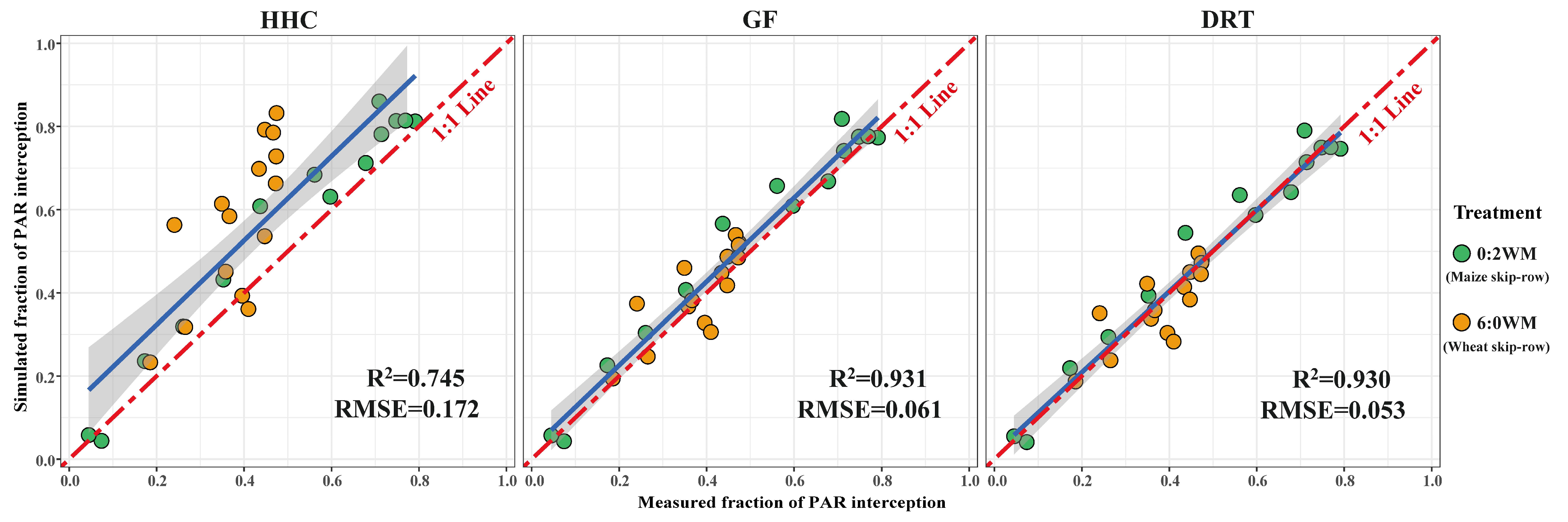
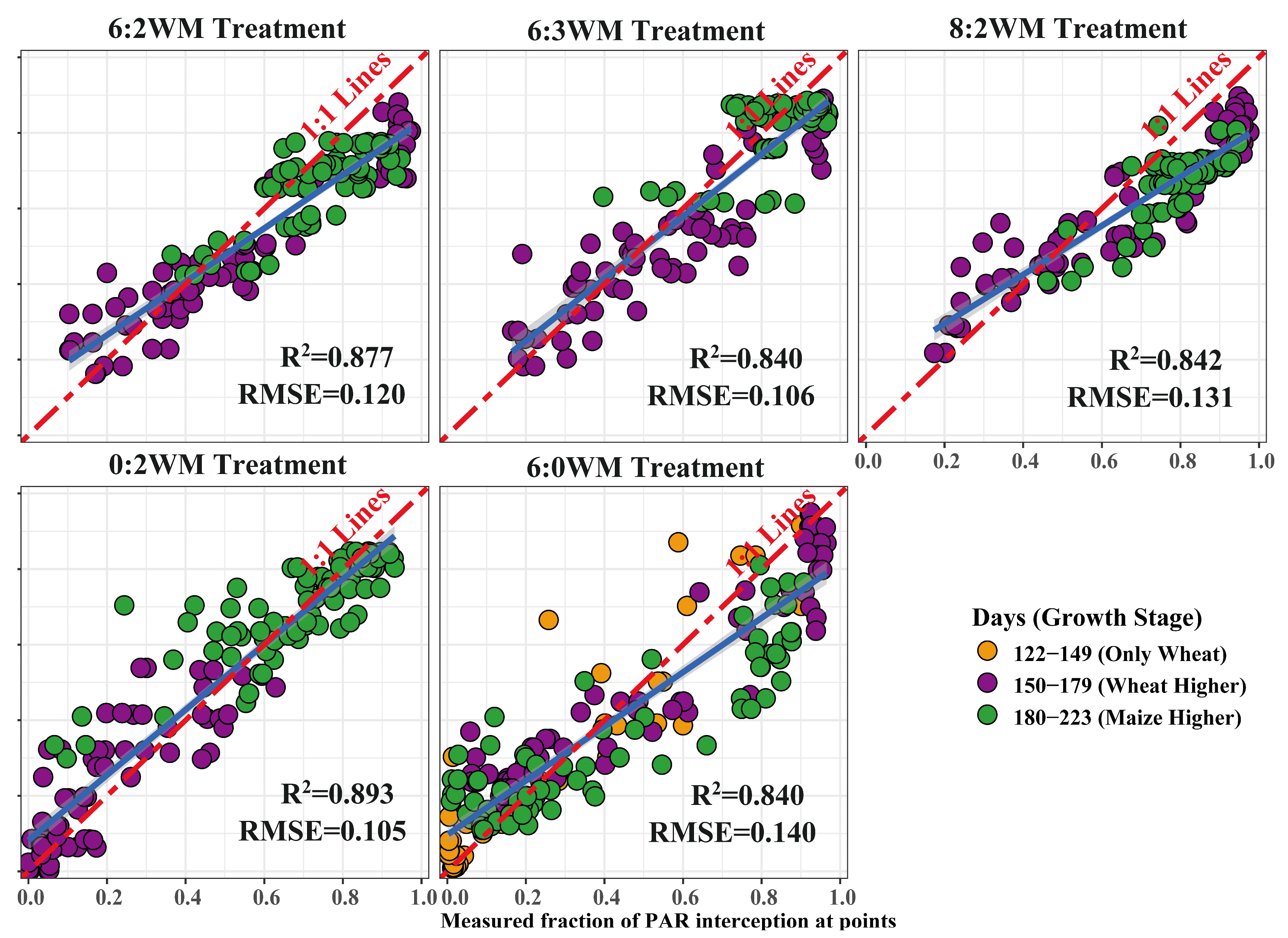
3.1.1. Fraction of Photosynthetically Active Radiation Interception

The simulated fraction of PAR interception in skip-row crop growth by the three models (HHC model, GF model, and DRT model) is shown in Table 1 and Figure 4. The calibrated parameters (Table 2) were determined according to Gou et al. [18], including the light extinction coefficient of two crops (kmaize = 0.69, kwheat = 0.63) and the strip width (d and p) in different intercropping ratios.
In the skip-row crop growth situation, the worst performances were obtained in the HHC model; the DRT model exhibited slight superiority over the GF model, with RMSE lower by 0.008. The simulated fraction of radiation interception by the HHC model was consistently greater than those of the GF model and DRT model. In the 0:2 WM treatment (maize skip-row), the simulated values of the three models exhibit little difference, ranging between 0 and 0.07. Additionally, the DRT model obtained higher accuracy than the GF model in the 0:2 WM treatment, with the RMSE lower by 0.01. In 6:0 WM (wheat skip-row), the HHC model obviously overestimates the fraction of radiation interception, while similar better performances were obtained in the GF and the DRT models.
In the two-crop co-growth situation (Table 3), the HHC model overestimates the PAR interception and exhibits the lowest simulation accuracy (R2 = 0.101, RMSE = 0.170). Moreover, the DRT model was superior to the GF model, with R2 higher by 0.042 and RMSE lower by 0.01. As shown in Figure 5, the simulated values of the DRT model were closer to the measured values than the GF model. Specifically, the simulated values of the GF model are greater than the DRT model during 143–154 days, while smaller than the GF model during 164–212 days. Additionally, the R2 of the DRT model in the 6:3 WM treatment (R2 = 0.962) was higher than that in the 6:2 WM (R2 = 0.925) and 8:2 WM (R2 = 0.908) treatments.

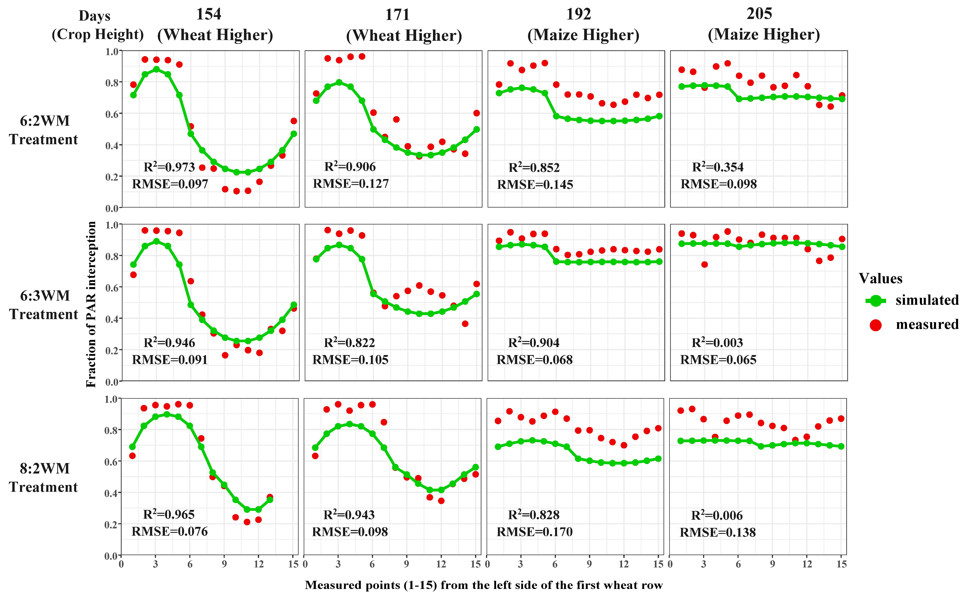
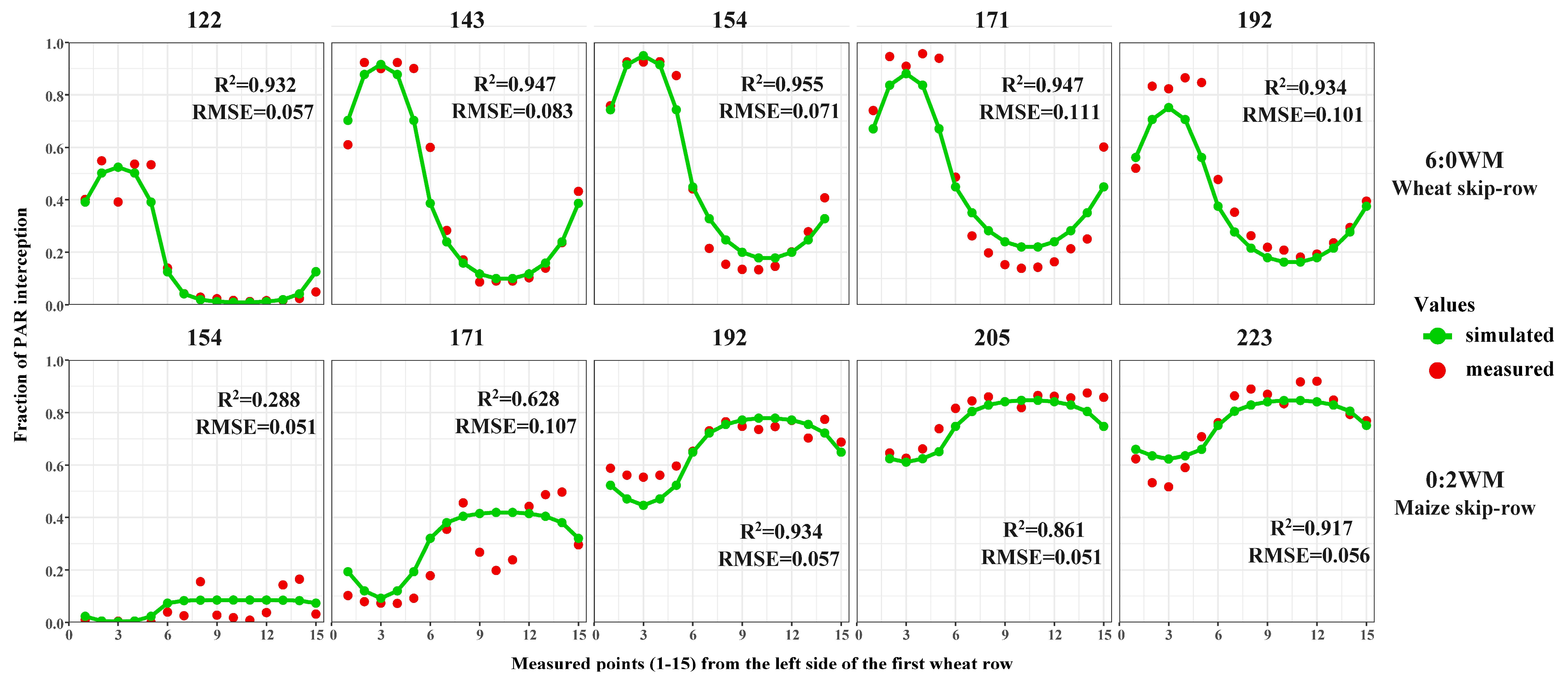
3.1.2. Simulated Spatiotemporal Photosynthetically Active Radiation Interception in the DRT Model

Figure 6 shows that the DRT model demonstrated satisfactory performance in simulating the fraction of PAR interception at measured points in different intercropping situations, with R2 ranging from 0.840 to 0.893 and RMSE ranging from 0.105 to 0.140. Specifically, Figure 7 shows the DRT model exhibited higher precision in simulating PAR interception at measured points during the period when wheat was taller than maize, such as on the 154th and 171st days, with R2 ranging from 0.822 to 0.973 and RMSE ranging from 0.076 to 0.127. On the 205th day, when maize was taller than wheat, the DRT model demonstrated lower R2 values but comparable RMSE values. Additionally, the DRT model shows the highest simulation accuracy in the 6:3 WM treatment (0.065 < RMSE < 0.105).
As shown in Figure 8, the DRT model showed high accuracy in simulating spatial PAR interception of the 6:0WM treatment (wheat skip-row) during the whole growth period, with R2 ranging from 0.932 to 0.955 and RMSE ranging from 0.057 to 0.111. The DRT model also performed excellently (0.861 < R2 < 0.934, RMSE < 0.057) in the later growth stages (such as days 192, 205, and 223) of the 0:2 WM treatment (maize skip-row). However, in the early growth stage of maize (days 154), the R2 was low. It is worth noting that, between days 154 and 171, the measured fraction of PAR interception showed two distinct peaks at the 8th and 13–14th measured points. Additionally, the DRT model aligns well with the growth and development of wheat and maize skip-row treatments.

3.2. Model Evaluation in Experiment B

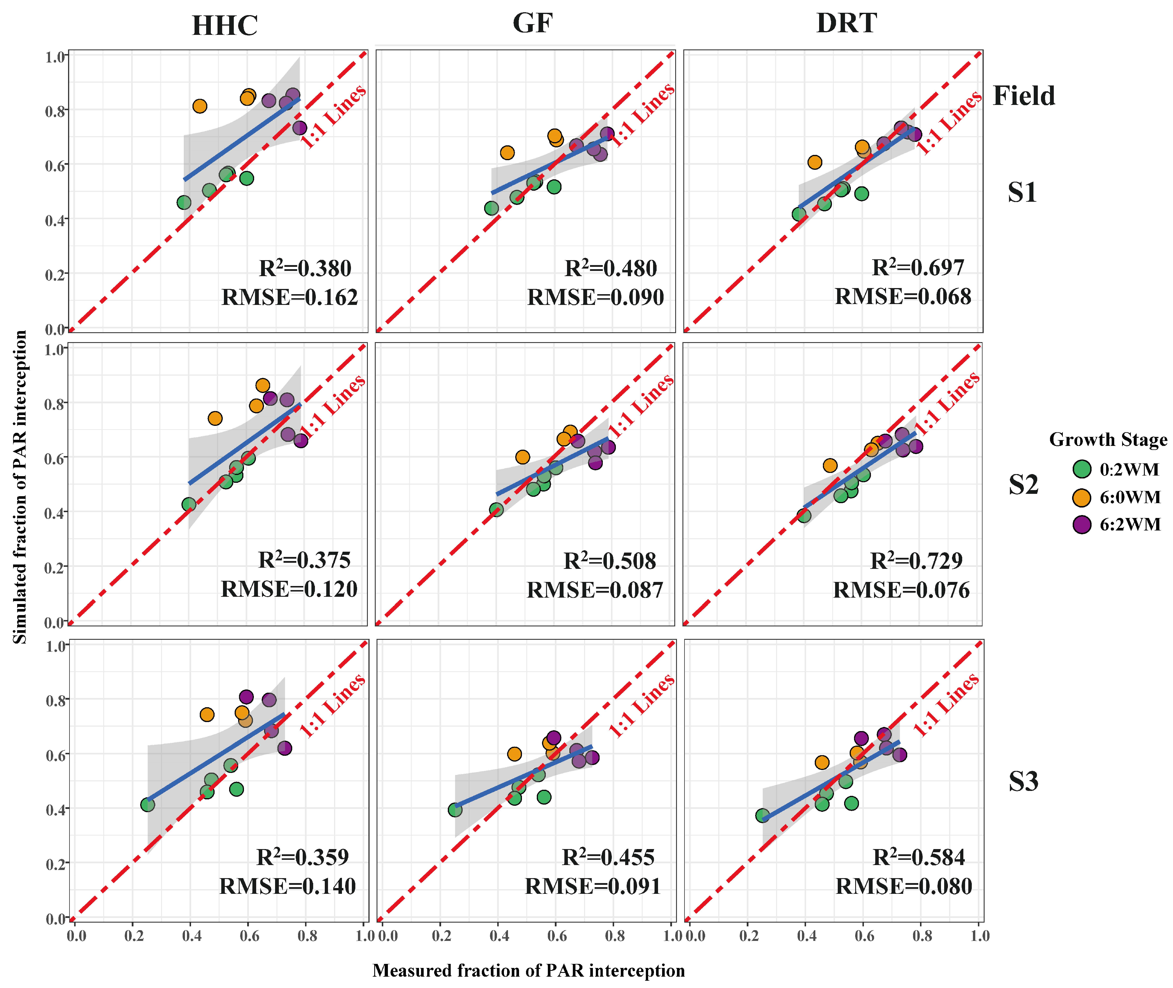
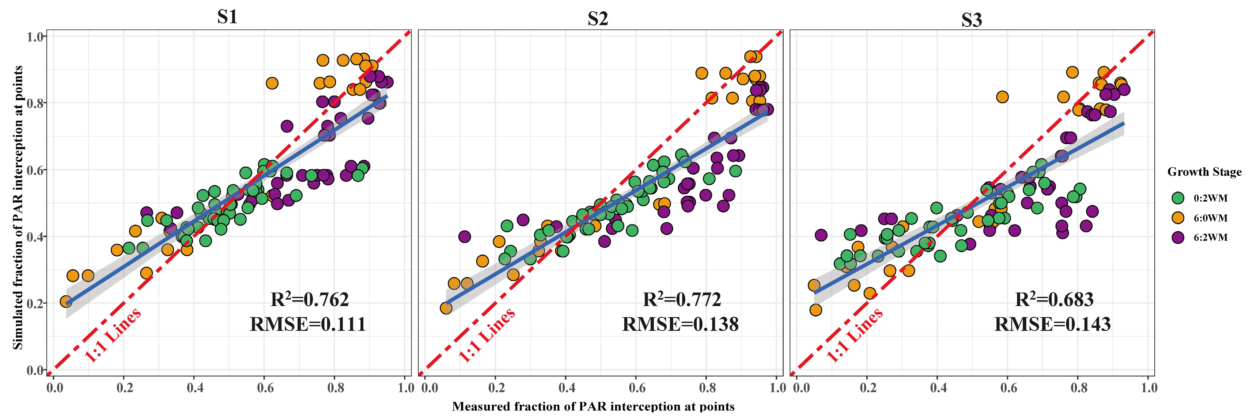
3.2.1. Fraction of Photosynthetically Active Radiation Interception

The measured and simulated fractions of radiation interception of the three models for skip-row crop growth are shown in Table 4 and Figure 9. The light extinction coefficients of wheat (kmaize) and maize (kwheat) were calibrated at 0.57 and 0.53, respectively. The strip width and path width (d and p) in Experiment B are in Table 5.
Compared with Experimental A, the performance of the three models exhibited a more significant disparity in Experimental B. In all fields with different salinity levels (S1, S2, S3), the DRT model outperformed the GF model with higher R2 (0.129–0.221) and lower RMSE (0.011–0.022), while the HHC model (0.359 < R2 < 0.380, 0.120 < RMSE < 0.162) exhibited the poorest performance (Figure 9). As shown in Table 4, although the GF model and the DRT model overestimated values on the 68th and 90th days (6:0 WM), the DRT model’s simulated values were relatively lower about 0.04 than those of the GF model. On the 105th and 139th days (6:2 WM), both of the two models were underestimated, while the DRT model’s simulated values were higher by approximately 0.06. Additionally, the simulation accuracy of both the GF and DRT models was slightly lower in the high-salinity field S3 (0.455 < R2 < 0.584) compared to the low-salinity field S1(0.480 < R2 < 0.697) and the medium-salinity field S2 (0.508 < R2 < 0.729).

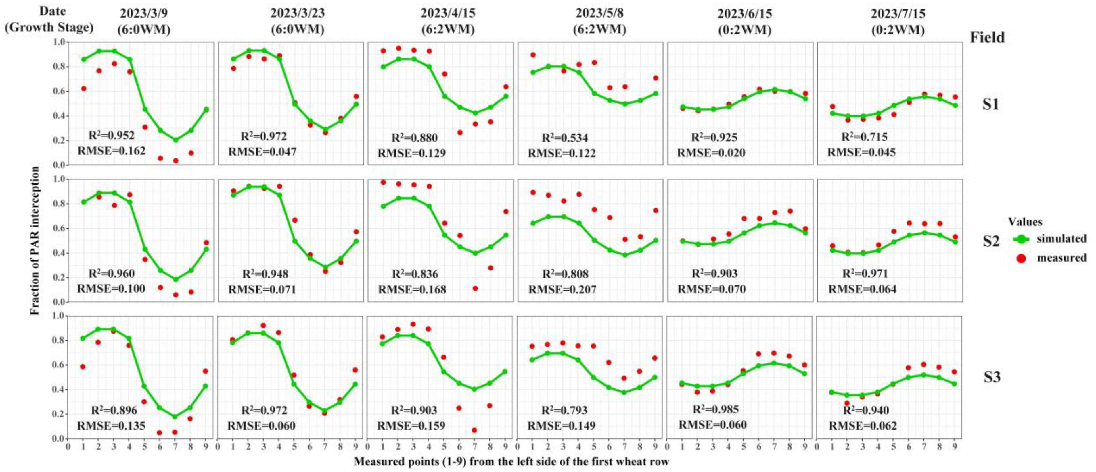
3.2.2. Simulated Spatiotemporal Photosynthetically Active Radiation Interception in the DRT Model

Compared with Experimental A (0.840 < R2 < 0.893), the DRT model exhibited a lower R2 in Experimental B (0.683–0.772) in the simulation of the fraction of PAR interception at measured points (Figure 10). Moreover, the accuracy of the DRT model is higher in low-salinity field S1 (R2 = 0.762, RMSE = 0.111) compared to its performance in high-salinity field S3 (R2 = 0.683, RMSE = 0.143). Additionally, the simulation results of DRT exhibit an overestimation within the 0.1–0.3 range while tending to underestimate within the 0.7–0.9 range. Figure 11 shows During the different growth stages, the accuracy of the DRT model is higher in crop skip-row growth (6:0 WM and 0:2 WM) than in the co-growth of wheat and maize (6:2 WM). The R2 of the 6:0 WM stage and the 0:2 WM stage is mainly larger than 0.9, and the RMSE is mainly lower than 0.1 in all fields. However, in the 6:2 WM stage (105th day), the simulated values were larger than the measured values at the 6–8 measured points. On the 128th day (6:2 WM), the simulated values were obviously larger than the measured values, with RMSE ranging from 0.122 to 0.207.

4. Discussion

4.1. The Factors Contributing to the Performances of the Three Models

This study evaluated the simulation performances of three statistical models in two distinct wheat-maize intercropping experiments. Experiment A was conducted in different intercropping configurations (strip width, sowing density, and sowing time). We intended to test the model’s accuracy under conditions without abiotic stress. Differently, Experiment B was conducted in different soil conditions (soil salinity) and focused on the model stability of varying growth conditions caused by salinity stress. Both experiments show the GF model obviously outperforms the HHC model (Figure 4, Figure 5, and Figure 9). The reason behind this is that the HHC model considers the strip intercropping canopy as a homogeneous canopy, ignoring light directly falling on the path, thereby overestimating simulated results [2,21]. Differently, the GF model applied a weighted average of the compressed canopy (w) into the strip intercropping to mitigate the overestimation. The GF model further quantifies the value of w based on the view factor theory by calculating the radiation interception along the strip and path.
Although the GF and DRT models both obtained acceptable simulation results, the DRT model exhibits superior accuracy and stability (higher R2 and lower RMSE) in Experiments A and B (Figure 4, Figure 5, and Figure 9). The lower simulation accuracy of the GF model could be attributed to it assuming that the indirect radiation completely passes through a homogenous canopy and ignoring the angular characteristics of the indirect radiation. But in practice, some of the indirect radiation traverses a small compressed canopy before reaching the soil surface, while other portions of indirect radiation need to pass through one or more compressed canopy before reaching the soil surface. Moreover, the radiation falling onto the strip and path may potentially be absorbed by both crops before reaching the soil surface. Different from the GF model, the DRT model employs both spatial and temporal integration using the Gaussian-Legendre methods for indirect radiation, enhancing model stability compared to the GF model. Such as during the period from the 68th to 128th days in the S1 field in Experiment B (Table 4), the simulated results of the DRT model were generally closer to the observed values. Furthermore, owing to its geometric structure, the DRT model provides more accurate radiation interception simulations for shorter crops compared to the GF model. In Experiment B, soil salinity influenced the model accuracy of both the DRT model and GF model, with lower accuracy observed in S3 compared with S1 and S2. This may be due to salinity stress impeding the growth of maize, restricting both plant height and LAI expansion, while the accuracy of radiation interception models relies on the assumption that the canopy is a rectangular hedge. Due to similar reasons, the R2 value of the DRT model in the 6:3 WM treatment, which increased the plant density of maize, is better than that of the 6:2 WM and 8:2 WM treatments. However, compared with the GF model, relatively satisfactory simulation performance in the high salinity field was obtained in the DRT model (R2 = 0.584, RMSE = 0.08), which indicates the adaptability of the DRT model in soil stress conditions. The DRT model is therefore well-suited for semi-arid regions characterized by elevated soil salinity levels, offering a viable alternative to the HHC model in both maize-bean and cereal-legume intercropping systems [10,25]. Additionally, the DRT model may be more suitable for soybean-maize intercropping systems compared to the HHC model and the GF model because it accommodates a longer co-growth period [2,26,27].

4.2. The Spatial Daily Radiation Interception of the DRT Model

Based on geometric principles, the DRT model simulates spatial variations of radiation interception in the intercropping system with few parameters (light extinction coefficient, LAI, width of strip, and path), which significantly reduces the computational complexity compared to the traditional geometric model [8]. Meanwhile, the simulations of the fraction of daily radiation interception at measured points by the DRT model generally exhibit relatively high accuracy and strong stability, with R2 values typically exceeding 0.85 and RMSE usually being less than 0.12.
However, it should be noted that the simulated spatial daily radiation interception in the DRT model is strictly symmetrical due to its simplifications of parameters and assumptions. This may result in a simulated range that is narrower than the observed range. Furthermore, both geometrical models and statistical models rely on a critical assumption; the crop canopy is assumed to be a chaotic rectangular hedge [9,15]. However, during the early growth stages of maize, the height and leaf area are small, the canopy does not completely cover the ground, and there are huge horizontal interspaces within the canopy structure, making it challenging for maize to meet the assumption of a whole rectangular canopy [28]. Therefore, the DRT model is challenging to simulate the two distinct peaks observed in the measured fraction of PAR interception at measured points, as shown on the 154th and 171st days of the 0:2 WM treatment (Figure 8), and restricted the model’s accuracy as demonstrated on the 128th day (Figure 11). But as maize grows and both plant height and LAI increase, the simulation accuracy of the DRT model is significantly improved.

5. Conclusions

This study developed a novel radiation interception model, the DRT model, for strip intercropping systems. The direct and indirect radiations were detailed and quantified using temporal and spatial integrations combined with the view factor theory. To access the model performances, the radiation interception of the wheat-maize intercropping system was simulated with the DRT model and the other two statistical models of HHC and GF in two distinct experiments. In both experiments, the DRT model outperformed the GF model and HHC model (higher R2 by 0.042–0.221 and lower RMSE by 0.008–0.022). In experiment A, the DRT model was slightly superior to the GF model in different intercropping configurations, with a lower RMSE of 0.008–0.01. In experiment B, the soil salinity may negatively affect the stability of the three models, causing a decrease in model accuracy. The DRT model showed stronger stability than the GF model and the HHC model (R2 higher by 0.129–0.221 and 0.225–0.354, respectively, and RMSE lower by 0.011–0.022 and 0.044–0.094, respectively). The DRT model offers a simple way to accurately describe the spatiotemporal radiation distribution of the strip intercropping system compared with the geometrical model. In the different treatments, the DRT model showed high accuracy and a strong ability to simulate the daily radiation distribution of experiment A (0.840 < R2 < 0.893, 0.105 < RMSE < 0.140) and experiment B (0.683 < R2 < 0.772, 0.111 < RMSE < 0.143). It is promising to couple the DRT model with the crop or soil physics models to explore the interactions among radiation utilization, water-heat-carbon cycle, crop growth, and yield formation of intercropping systems in diverse environments.

Author Contributions

Conceptualization, L.D., Y.L. and W.Z.; methodology, L.D., Y.L. and G.L.; software, L.D. and Y.L.; validation, L.D.; formal analysis, L.D. and G.L.; writing—original draft preparation, L.D.; writing—review and editing, G.L. and W.Z.; visualization, L.D. and G.L.; supervision, J.H., W.Z. and G.L.; funding acquisition, W.Z. and G.L. All authors have read and agreed to the published version of the manuscript.

Funding

This research was funded by the National Key Research and Development Program of China (Grant No. 2021YFD1900805-03), National Natural Science Foundation of China (NSFC) (Grant Nos. 52379045, 52209066, 52179039), the China Postdoctoral Science Foundation funded project (No. 2020M682475), the fundamental research funds for the central universities (Grant No. 2042021kf0051).

Data Availability Statement

Data will be made available on request.

Conflicts of Interest

The authors declare no conflict of interest.

Appendix A

According to the view factor theory, Ip,d and Id,d can be calculated as follows:
I p , d = 2 0 p θ 1 π 2 sin θ d θ d x 2 0 d + p 0 π 2 sin θ d θ d x = 0 p x x 2 + h 2 d x ( p + d ) = p 2 + h 2 h p + d
I d , d = e k · L A I c d 2 + h 2 h d + p
where x represents an arbitrary point within the space integration; θ1 is the angle of the view factor at that specific point; LAIc is the LAI of the compressed canopy, calculated as follows:
L A I c = L A I · p + d d
The indirect radiation can be calculated based on the geometric relationships of the incident light angles. As shown in Figure A1, the incident angles (θ) relate to the number of intercropping units (i). Thus, when the incident light angle is between θ2i−1 and θ2i+1, the LAI of the compressed canopy is calculated as follows:
L A I 1 = L A I c · h · cot θ x i 1 p h · cot θ
L A I 2 = L A I c · i · d h · cot θ
where LAI1 is the LAI of the compressed canopy with accordingly vertical thickness when θ between θ2i and θ2i−1, and LAI2 is when θ between θ2i and θ2i+1. Thus, from θ2i−1 to θ2i+1, the indirect radiation at the point P on the path (rpx(θi)) is calculated by angle integration as follows:
r p x θ i = θ 2 i θ 2 i 1 e k · L A I 1 · sin θ d θ + θ 2 i + 1 θ 2 i e k · L A I 2 · sin θ d θ
Then, the total indirect radiation at the point P, rp(x), is the sum of rpx(θi) in each intercropping unit. Considering the critical angle θ2i+1 approaches 0 but never reaches 0, we add a residual term for the angle integration from 0 to the last θ2i+1. In this study, the value of I was set to 3 to balance the accuracy and computations.
Figure A1. Diagram of the geometric structure of the crop skip-row growth in the strip intercropping system. (P is an arbitrary point on the path; i represents the i-th intercropping unit undergoing calculation; θ2i−1, θ2i, and θ2i+1 are the critical angle of the incident light; when incident light angle θ is between θ2i−1 and θ2i+1, radiation will reach point P through i intercropping units to reach point P).
Agronomy 14 00227 g0a1
r p x = r p x θ 1 + r p x θ 2 + + r p x θ i + e k · L A I · 1 cos θ 2 i + 1
I p , i = 0 p r p ( x )   d x d + p
From Equations (A6) and (A8), due to the functional relationship between LAI1/ LAI2 and θ, rpx(θi) represent an indefinite integral, we employ the approach used in geometrical models and apply the Gaussian integration to numerically approximate the indefinite integral [29]. In addition, the integrand is a monotonic function represented by a smooth curve, which satisfies the requirements of Gaussian integration [9]. For example, the angle integration in Equation (A6) and the space integration in Equation (A8) can be calculated by 8-point Gaussian integration as follows:
θ 2 i θ 2 i 1 e k · L A I 1 · sin θ d θ = n = 1 8 w n · θ 2 i 1 θ 2 i · e k · L A I 1 · sin θ 2 i + a n θ 2 i 1 θ 2 i
0 p r p ( x )   d x = n = 1 8 w n · p · r p ( a n p )
where an is the Gaussian point, a1–a8 is (0.0199, 0.1017, 0.2372, 0.4083, 0.5917, 0.7628, 0.8983, 0.9801); wn is the weight of the selected point, w1–w8 is (0.0506, 0.1112, 0.1569, 0.1883, 0.1883, 0.1569, 0.1112, 0.0506). In Equation (A9), LAI1 is also the function of θ which needs to be replaced by θ2i+ an(θ2i−1θ2i).
Then, Ip,i can be calculated. The calculation of Id,i follows the same method as the calculation of Ip,i:
L A I 2 = L A I c · h · cot θ i · p h · cot θ
L A I 1 = L A I c · x + i 1 d h · cot θ
r d x θ i = θ 2 i θ 2 i 1 e k · L A I 1 · sin θ d θ + θ 2 i + 1 θ 2 i e k · L A I 2 · sin θ d θ
I d , i = 0 d r d ( x )   d x d + p
Above all, the radiation interception of the single crop (f) can be calculated.

Appendix B

The calculation method for the direct radiation of both crops is consistent with that employed in Appendix A. The LAI of the compressed canopy of crop 1 (LAI1,c) and crop 2 (LAI2,c) is calculated as follows:
L A I 1 , c = L A I 1 · d + p d
L A I 2 , c = L A I 2 · d + p p
Then, the direct radiation (through the canopy) that falls on the soil surface of p (Ip,d) and d (Id,d), and the direct radiation intercepted by Crop 1 (F1d,d) and Crop 2 (F2p,d) can be quantified as follows:
I p , d = e k 2 · L A I 2 , c p 2 + h 1 2 h 1 d + p
I d , d = e k 1 · L A I 1 , c d 2 + h 1 2 h 1 d + p
F 1 d , d = 1 e k 1 · L A I 1 , c · d 2 + h 1 2 h 1 p + d
F 2 p , d = 1 e k 2 · L A I 2 , c · p 2 + h 1 2 h 1 p + d
In two-crop co-growth situations, the radiation is successively intercepted by the two crops. The calculation of indirect radiation needs to be performed sequentially at several intercropping units. The radiation emitted from the previous intercropping unit is the incident radiation received by the subsequent intercropping unit. Figure A2 illustrates the indirect radiation entering from the i-th intercropping unit and eventually falling on the strip of the shorter crop (p).
Figure A2. Diagram of the geometric structure of the co-growth of two crops in a strip intercropping system. The parameters have the same meanings as those in Figure A1.
Agronomy 14 00227 g0a2
When light enters an intercropping unit, regardless of whether θ is between θ2i+1 and θ2i or between θ2i and θ2i−1, the light passes through the area of shorter crops (crop 2) before traversing the area of taller crops (crop 1). Therefore, it is necessary to determine whether the light passes through the compressed canopy of crop 2. By comparing the vertical projection of the light incident point and light outgoing point with the height of crop 2, we can calculate the radiation interception. The method is the analogy to Liu, Chen, Li, Guo, Tian, Yao and Lin [8], as Figure A3 shown.
Figure A3. The three relationships between the vertical projection of light incident and outgoing points of the taller crop canopy and the height of the shorter crop.
Agronomy 14 00227 g0a3
When 0 < n ≤ i:
h ( x ) n , 1 = x + n · p + d · tan θ
h x n , 2 = x + n 1 · p + n · d · tan θ
L A I 2 , n = L A I 2 , c · p h 2 · cot θ h 2 h x n , 1 > h x n , 2 L A I 2 , c p h 2 · cot θ · h 2 h x n , 2 h x n , 1 h x n , 2 h x n , 1 > h 2 > h x n , 2 0 h 2 h x n , 2
When n = 0:
h ( x ) 0 = x · tan θ
L A I 2 , 0 = L A I 2 , c h ( x ) 0 h 2 L A I 2 , c · h ( x ) 0 h 2 h ( x ) 0 < h 2
where i represents how many complete intercropping units (left of point P) have been passed through by the light, and n represents the n-th intercropping unit to the left of point P where the light is passing through; in the computation of LAI2,n, n can be categorized into two scenarios: n = 0 and 0 < ni. The h(x)n,1 and h(x)n,2 are the heights of the light incident point and light outgoing point in the n-th intercropping unit, respectively. LAI2,n is the LAI of the compressed canopy with accordingly vertical thickness in the n-th intercropping unit. In the computation of LAI1,n, and n needs to be categorized into three scenarios: n = i, 0 < n < i, and n = 0:
L A I 1 , n = L A I 1 , c h 1 · cot θ x i 1 d i 1 p h 1 · cot θ           n = i L A I 1 , c d h 1 · cot θ           0 < n < i 0                     n = 0
When point P is on the strip of the shorter crop (p), the light inevitably traverses the area occupied by the shorter crop (p) before traversing the area occupied by the taller crop (d). Consequently, it becomes necessary to compute the radiation interception of the two crops sequentially, following the order of intercropping units and the hierarchy of the two crops. Unlike Module 1, it is imperative to calculate the radiation interception separately for each crop within every intercropping unit in Module 2. Therefore, the computation will initiate from n = i, followed by a decrement of 1 for each subsequent iteration, until the calculation concludes at n = 0. According to Beer’s law, the radiation interception by crop 2 and crop 1 at the point P is calculated as follows:
s u m i + 1 = 0
s u m n = s u m n + 1 + k 2 · L A I 2 , n + k 1 · L A I 1 , n
A 2 θ i , n = e s u m n + 1 e s u m n + 1 + k 2 · L A I 2 , n
A 1 θ i , n = e s u m n + 1 + k 2 · L A I 2 , n e s u m n + 1 + k 2 · L A I 2 , n + k 1 · L A I 1 , n
r p x 2 θ i = θ 2 i + 1 θ 2 i 1 sin θ · n = 0 i A 2 θ , n d θ
r p x 1 θ i = θ 2 i + 1 θ 2 i 1 sin θ · n = 0 i A 1 θ , n d θ
where sumn refers to the accumulated vegetation transmittance after the n-th intercropping unit, sumi+1 is the initial value for iteration as 0; A2(θ,n) and A1(θ,n) are the proportions of radiation intercepted by crop 1 and crop 2, respectively, within the n-th intercropping unit. The Equations (A29) and (A30) indicate the light passes through the region of Crop2 before traversing the region of crop 1 when point P is on the strip of crop 2 (p). The rpx1(θ) and rpx2(θ) are the radiation interceptions of crop 1 and crop 2, respectively, at point P. By spatial integration, we can obtain the indirect radiation intercepted by crop 1 and crop 2 along the strip of the shorter crop:
F 1 p , i = 0 p i = 1 i r p x 1 θ i d x
F 2 p , i = 0 p i = 1 i r p x 2 θ i d x
where F1p,i and F2p,i are the indirect radiation interception of crop 1 and crop 2 along the strip of the shorter crop (p), respectively. The indefinite integration in Equations (A31)–(A34) is calculated by the 8-point Gaussian integration, similar to that employed in module 1.
Similarly, the indirect radiation interception of crop 1 and crop 2 along the strip of the taller crop (d) is calculated in the same way. However, there are several differences. First, due to the location of an integrated point on the strip of crop 1 (d), the calculation for h(x)n,1 and h(x)n,1 has been modified, while the calculation for LAI2,n remains the same with Equation (A23):
When 0 < ni:
h ( x ) n , 1 = x + n · p + n 1 · d · tan θ
h x n , 2 = x + n 1 · p + d · tan θ
L A I 2 , n = L A I 2 , c · p h 2 · cot θ             h 2 h x n , 1 > h x n , 2 L A I 2 , c p h 2 · cot θ · h 2 h x n , 2 h x n , 1 h x n , 2         h x n , 1 > h 2 > h x n , 2 0                         h 2 h x n , 2
When n = 0:
L A I 2 , 0 = 0
Secondly, the calculation method for LAI1,n varies across different intercropping units (different n) and has differences during angle integration as follows:
When angle integration is from θ2i to θ2i−1:
L A I 1 , n = L A I 1 , c h 1 · cot θ x i 1 d i · p h 1 · cot θ         n = i L A I 1 , c d h 1 · cot θ             0 < n < i L A I 1 , c x h 1 · cot θ             n = 0
When angle integration is from θ2i+1 to θ2i:
L A I 1 , n = 0 n = i L A I 1 , c d h 1 · cot θ 0 < n < i L A I 1 , c x h 1 · cot θ n = 0
Thirdly, when the integrated point is on the strip of crop 2 (p), the light first traverses the region of crop 2 before passing through the region of crop 1. On the opposite, when the integrated point is on the strip of crop 1 (d), the light first traverses the region of crop 1 before passing through the region of crop 2, just like the following Equations (A41) and (A42) show:
A 1 θ i , n = e s u m n + 1 e s u m n + 1 + k 1 · L A I 1 , n
A 2 θ i , n = e s u m n + 1 + k 1 · L A I 1 , n e s u m n + 1 + k 2 · L A I 2 , n + k 1 · L A I 1 , n
The other steps, such as angle integration and space integration, are totally the same:
r p x 1 θ i = θ 2 i + 1 θ 2 i 1 sin θ · n = 0 i A 1 θ , n d θ
r p x 2 θ i = θ 2 i + 1 θ 2 i 1 sin θ · n = 0 i A 2 θ , n d θ
F 1 d , i = 0 d i = 1 i r p x 1 θ i d x
F 2 d , i = 0 d i = 1 i r p x 2 θ i d x
where F1d,i and F2d,i are the indirect radiation interception of crop 1 and crop 2 along the strip of the taller crop (d), respectively. The indefinite integration in Equations (A43)–(A46) is calculated by the 8-point Gaussian integration, similar to that employed in module 1.

Appendix C

The Module 3 of the DRT model has 2 steps:
First, due to the position of simulated points (x) controlled by the position of Gaussian points (an), it is necessary to ensure the alignment between the positions of the Gaussian points and the measured PAR points. For example, when we calculate the light interception of the measured points located on the strip of wheat (d = 75 cm, 5 measured points), it must use 5-point Gaussian integration for the 5 measured points. When we calculate the points located on the strip of maize (p = 150 cm, 10 measured points), we use 10-point Gaussian integration for the 10 measured points on the strip. In the Wuhan University experiment, it used 4-point Gaussian integration in the strip of wheat and 5-point Gaussian integration in the strip of maize (a total of 9 measured points). Then, the spacing between measurement points aligns with the spacing of model simulation points, and the positions of the experimentally measured points correspond to the positions of the simulated Gaussian points.
Secondly, unlike calculating the total direct radiation interception on the strip, it is necessary to calculate the light interception of the direct radiation at every Gaussian point. The calculation of the indirect radiation (rp(x) and rd(x)) in Module 3 is identical to Module 1 and Module 2.

References

  1. Mao, L.L.; Zhang, L.Z.; Zhang, S.P.; Evers, J.B.; van der Werf, W.; Wang, J.J.; Sun, H.Q.; Su, Z.C.; Spiertz, H. Resource use efficiency, ecological intensification and sustainability of intercropping systems. J. Integr. Agric. 2015, 14, 1542–1550. [Google Scholar] [CrossRef]
  2. Wu, Y.S.; He, D.; Wang, E.L.; Liu, X.; Huth, N.I.; Zhao, Z.G.; Gong, W.Z.; Yang, F.; Wang, X.C.; Yong, T.W.; et al. Modelling soybean and maize growth and grain yield in strip intercropping systems with different row configurations. Field Crop. Res. 2021, 265, 108122. [Google Scholar] [CrossRef]
  3. Du, J.B.; Han, T.F.; Gai, J.Y.; Yong, T.W.; Sun, X.; Wang, X.C.; Yang, F.; Liu, J.; Shu, K.; Liu, W.G.; et al. Maize-soybean strip intercropping: Achieved a balance between high productivity and sustainability. J. Integr. Agric. 2018, 17, 747–754. [Google Scholar] [CrossRef]
  4. Yang, F.; Liao, D.P.; Wu, X.L.; Gao, R.C.; Fan, Y.F.; Raza, M.A.; Wang, X.C.; Yong, T.W.; Liu, W.G.; Liu, J.; et al. Effect of aboveground and belowground interactions on the intercrop yields in maize-soybean relay intercropping systems. Field Crops Res. 2017, 203, 16–23. [Google Scholar] [CrossRef]
  5. Lemeur, R.; Blad, B.L. A critical review of light models for estimating the shortwave radiation regime of plant canopies. Agric. Meteorol. 1974, 14, 255–286. [Google Scholar] [CrossRef]
  6. Nilson, T. Radiative Transfer in Nonhomogeneous Plant Canopies. In Advances in Bioclimatology 1; Desjardins, R.L., Gifford, R.M., Nilson, T., Greenwood, E.A.N., Eds.; Springer: Berlin/Heidelberg, Germany, 1992; pp. 59–88. [Google Scholar]
  7. Wang, Z.; Zhao, X.; Wu, P.; Gao, Y.; Yang, Q.; Shen, Y. Border row effects on light interception in wheat/maize strip intercropping systems. Field Crops Res. 2017, 214, 1–13. [Google Scholar] [CrossRef]
  8. Liu, H.T.; Chen, S.H.; Li, B.G.; Guo, S.; Tian, J.; Yao, L.; Lin, C.W. The effect of strip orientation and width on radiation interception in maize-soybean strip intercropping systems. Food Energy Secur. 2022, 11, e364. [Google Scholar] [CrossRef]
  9. Gijzen, H.; Goudriaan, J. A flexible and explanatory model of light-distribution and photosynthesis in row crops. Agric. For. Meteorol. 1989, 48, 1–20. [Google Scholar] [CrossRef]
  10. Tsubo, M.; Walker, S. A model of radiation interception and use by a maize-bean intercrop canopy. Agric. For. Meteorol. 2002, 110, 203–215. [Google Scholar] [CrossRef]
  11. Munz, S.; Graeff-Honninger, S.; Lizaso, J.I.; Chen, Q.; Claupein, W. Modeling light availability for a subordinate crop within a strip-intercropping system. Field Crop. Res. 2014, 155, 77–89. [Google Scholar] [CrossRef]
  12. Wang, Z.K.; Cao, Q.; Shen, Y.Y. Modeling light availability for crop strips planted within apple orchard. Agric. Syst. 2019, 170, 28–38. [Google Scholar] [CrossRef]
  13. OzierLafontaine, H.; Vercambre, G.; Tournebize, R. Radiation and transpiration partitioning in a maize-sorghum intercrop: Test and evaluation of two models. Field Crops Res. 1997, 49, 127–145. [Google Scholar] [CrossRef]
  14. Goudriaan, J. Crop Micrometeorology: A Simulation Study; Wageningen University and Research: Wageningen, The Netherlands, 1977. [Google Scholar]
  15. Pronk, A.A.; Goudriaan, J.; Stilma, E.; Challa, H. A simple method to estimate radiation interception by nursery stock conifers: A case study of eastern white cedar. NJAS Wagening. J. Life Sci. 2003, 51, 279–295. [Google Scholar] [CrossRef]
  16. Zhang, L.; van der Werf, W.; Bastiaans, L.; Zhang, S.; Li, B.; Spiertz, J.H.J. Light interception and utilization in relay intercrops of wheat and cotton. Field Crops Res. 2008, 107, 29–42. [Google Scholar] [CrossRef]
  17. Wang, Z.K.; Zhao, X.N.; Wu, P.T.; He, J.Q.; Chen, X.L.; Gao, Y.; Cao, X.C. Radiation interception and utilization by wheat/maize strip intercropping systems. Agric. For. Meteorol. 2015, 204, 58–66. [Google Scholar] [CrossRef]
  18. Gou, F.; van Ittersum, M.K.; Simon, E.; Leffelaar, P.A.; van der Putten, P.E.L.; Zhang, L.; van der Werf, W. Intercropping wheat and maize increases total radiation interception and wheat RUE but lowers maize RUE. Eur. J. Agron. 2017, 84, 125–139. [Google Scholar] [CrossRef]
  19. Berghuijs, H.N.C.; Weih, M.; van der Werf, W.; Karley, A.J.; Adam, E.; Villegas-Fernandez, A.M.; Kiaer, L.P.; Newton, A.C.; Scherber, C.; Tavoletti, S.; et al. Calibrating and testing APSIM for wheat-faba bean pure cultures and intercrops across Europe. Field Crop. Res. 2021, 264, 108088. [Google Scholar] [CrossRef]
  20. Van Oort, P.A.J.; Gou, F.; Stomph, T.J.; van der Werf, W. Effects of strip width on yields in relay-strip intercropping: A simulation study. Eur. J. Agron. 2020, 112, 125936. [Google Scholar] [CrossRef]
  21. Gou, F.; van Ittersum, M.K.; van der Werf, W. Simulating potential growth in a relay-strip intercropping system: Model description, calibration and testing. Field Crops Res. 2017, 200, 122–142. [Google Scholar] [CrossRef]
  22. Pinto, V.M.; van Dam, J.C.; van Lier, Q.D.; Reichardt, K. Intercropping Simulation Using the SWAP Model: Development of a 2×1D Algorithm. Agriculture 2019, 9, 126. [Google Scholar] [CrossRef]
  23. Pierre, J.F.; Singh, U.; Ruiz-Sánchez, E.; Pavan, W. Development of a Cereal-Legume Intercrop Model for DSSAT Version 4.8. Agriculture 2023, 13, 845. [Google Scholar] [CrossRef]
  24. Holzworth, D.P.; Huth, N.I.; Devoil, P.G.; Zurcher, E.J.; Herrmann, N.I.; McLean, G.; Chenu, K.; van Oosterom, E.J.; Snow, V.; Murphy, C.; et al. APSIM—Evolution towards a new generation of agricultural systems simulation. Environ. Model. Softw. 2014, 62, 327–350. [Google Scholar] [CrossRef]
  25. Tsubo, M.; Walker, S.; Ogindo, H.O. A simulation model of cereal–legume intercropping systems for semi-arid regions. Field Crop. Res. 2005, 93, 10–22. [Google Scholar] [CrossRef]
  26. Gao, Y.; Duan, A.W.; Qiu, X.Q.; Li, X.Q.; Pauline, U.; Sun, J.S.; Wang, H.Z. Modeling evapotranspiration in maize/soybean strip intercropping system with the evaporation and radiation interception by neighboring species model. Agric. Water Manag. 2013, 128, 110–119. [Google Scholar] [CrossRef]
  27. Li, S.W.; van Der Werf, W.; Zhu, J.Q.; Guo, Y.; Li, B.G.; Ma, Y.T.; Evers, J.B. Estimating the contribution of plant traits to light partitioning in simultaneous maize/soybean intercropping. J. Exp. Bot. 2021, 72, 3630–3646. [Google Scholar] [CrossRef]
  28. Stewart, D.W.; Costa, C.; Dwyer, L.M.; Smith, D.L.; Hamilton, R.I.; Ma, B.L. Canopy structure, light interception, and photosynthesis in maize. Agron. J. 2003, 95, 1465–1474. [Google Scholar] [CrossRef]
  29. Goudriaan, J. A simple and fast numerical-method for the computation of daily totals of crop photosynthesis. Agric. For. Meteorol. 1986, 38, 249–254. [Google Scholar] [CrossRef]
Figure 1. Diagram depicting the canopy structure of a homogeneous canopy, a strip-planted canopy, and a compressed canopy.
Agronomy 14 00227 g001
Figure 2. Diagram depicting the angular relationships and distance for direct radiation of crop skip-row growth and co-growth of two crops. It is a symmetrical pattern, which means the sum of the angle integrations from θ1 to π/2 for two symmetrical points is equal to the integration from θ1 to θ2 for either of them. Crop 1 is the taller crop while crop 2 is the shorter crop of the intercropping system; P is an arbitrary point on the path or strip; x is the distance from point P to the left edge of the hedge; h is the plant height (h1 and h2 correspond to crop 1 and crop 2); d is the strip width (the strip width of crop 1 in subplot B); p is the path width (the strip width of crop 2 in subplot B).
Agronomy 14 00227 g002
Figure 3. Treatment 1 is a sole wheat crop sown at a 15 cm row distance. Treatment 2 is a sole maize crop sown at a 40 cm row distance. Treatment 3 is a wheat-maize intercrop comprising two rows of maize and six rows of wheat with the same row spacing as Treatment 1 and Treatment 2. Treatment 3 had three growth stages, including wheat skip-row growth (6:0 WM, from days 68 to 91), co-growth (6:2 WM, from days 92 to 151), and maize skip-row growth (6:0 WM, from days 152 to 213). The red points (1−9) in treatment 3 represent the positions where the SunScan probe was placed parallel to the rows.
Agronomy 14 00227 g003
Figure 4. The scatterplots of measured and simulated fraction of PAR interception generated from the three models at crop skip-row growth (6:0 WM and 0:2 WM).
Agronomy 14 00227 g004
Figure 5. The scatterplots of measured and simulated fraction of PAR interception generated from the three models at co-growth of two crops (6:2 WM, 6:3 WM, and 8:2 WM).
Agronomy 14 00227 g005
Figure 6. The scatterplots of measured and simulated fractions of PAR interception at measured points by the DRT model of different treatments during three growth stages.
Agronomy 14 00227 g006
Figure 7. Comparison of simulated versus measured daily fractions of PAR interception at 15 measured points of three treatments by the DRT model. Days 154, 171, 192, and 205 were selected to show the modeling accuracy in different growth stages.
Agronomy 14 00227 g007
Figure 8. Comparison of simulated versus measured daily fractions of PAR interception at 15 measured points of 6:0 WM treatment and 0:2 WM treatment by the DRT model. Days 154, 171, 192, 205, and 223 for 6:0 WM and days 122, 143, 154, 171, and 192 for 0:2 WM were selected to show the modeling accuracy in different growth stages.
Agronomy 14 00227 g008
Figure 9. The scatterplots of measured and simulated fraction of PAR interception generated from the three models at different fields (S1, S2, S3) during three growth stages (6:0 WM, 6:2 WM, and 0:2 WM).
Agronomy 14 00227 g009
Figure 10. The scatterplots of measured and simulated fraction of PAR interception at measured points by the DRT model at different fields (S1, S2, and S3) during three growth stages (6:0 WM, 6:2 WM, and 0:2 WM).
Agronomy 14 00227 g010
Figure 11. Comparison of simulated versus measured daily fractions of PAR interception at nine measured points during different growth stages of three fields by the DRT model. Days 68, 82, 105, 128, 166, and 196 were selected to show the modeling accuracy in different growth stages.
Agronomy 14 00227 g011
Table 1. The measured and simulated fraction of PAR interception of the three models at crop skip-row growth.
TreatmentDaysMeasuredHHCGFDRT
0:2 WM1500.0740.0440.0430.041
1540.0450.0580.0570.055
1640.1730.2360.2260.219
1710.2610.3190.3040.294
1780.3530.4320.4070.393
1840.4370.6080.5660.544
1920.6780.7120.6680.642
1990.7140.7810.7410.714
2050.7910.8120.7730.746
2120.7480.8130.7750.749
2230.7690.8140.7760.750
223 (6:2 WM)0.5610.6840.6570.635
223 (6:3 WM)0.7090.8600.8180.790
223 (8:2 WM)0.5970.6310.6090.587
6:0 WM1220.1850.2330.1940.187
1360.2410.5630.3740.351
1430.4340.6980.4480.414
1500.4470.7920.4870.450
1540.4740.8320.5200.479
1640.4670.7850.5390.495
1710.4730.7280.5150.472
1780.4720.6630.4850.445
1840.3490.6140.4600.422
1920.4470.5360.4180.384
1990.3580.4510.3670.338
2050.3960.3930.3280.304
2120.4100.3610.3060.283
122 (8:2 WM)0.2650.3180.2470.238
136 (8:2 WM)0.3660.5840.3820.358
R2 -0.7450.9310.930
RMSE -0.1720.0610.053
Table 2. The strip width of different treatments as model input parameter.
TreatmentCrop Heightd (cm)p (cm)
0:2 WMMaize skip-row15075
6:0 WMWheat skip-row75150
6:2 WMW higher M75150
M higher W15075
6:3 WMW higher M75150
M higher W15075
8:2 WMW higher M100125
M higher W125100
Table 3. The measured and simulated fraction of PAR interception of the three models at the co-growth of two crops.
Crop HeightTreatmentDaysMeasuredHHCGFDRT
W higher M6:2 WM1430.4340.6810.4640.438
1500.5010.7730.5210.502
1540.4780.8130.5620.544
1640.5430.7760.5820.588
1710.5990.7420.5840.610
1780.6060.7320.6380.667
6:3 WM1430.4340.6980.4880.461
1500.5430.7970.5660.545
1540.5160.8380.6150.595
1640.5790.8320.6590.665
1710.6600.8290.6880.712
1780.7590.8430.7660.788
8:2 WM1430.5600.7370.5400.522
1500.5850.8350.5980.591
1540.6160.8740.6370.630
1640.6610.8480.6400.669
1710.6610.8210.6430.684
1780.7370.7980.6790.719
M higher W6:2 WM1840.6220.7320.6840.712
1920.7670.7370.7200.742
1990.7370.7460.7300.763
2050.7950.7590.7410.781
2120.7770.7550.7360.781
6:3 WM1840.7490.8490.8190.838
1920.8590.8660.8490.869
1990.8490.8830.8570.886
2050.8820.8980.8660.898
2120.8900.8960.8640.897
8:2 WM1840.7300.7710.6540.706
1920.8130.7470.7380.753
1990.8110.7370.7230.753
2050.8430.7480.7280.766
2120.8280.7350.7140.758
R2 -0.1010.8520.894
RMSE -0.1700.0550.045
Table 4. The measured and simulated fractions of PAR interception of the three models at different growth stages.
FieldDays (Stage)MeasuredHHCGFDRT
S168 (6:0 WM)0.4360.8120.6410.606
82 (6:0 WM)0.6060.8510.6880.647
90 (6:0 WM)0.6000.840.7030.662
105 (6:2 WM)0.6750.8320.6670.674
116 (6:2 WM)0.7580.8530.6350.717
128 (6:2 WM)0.7350.8230.6550.732
139 (6:2 WM)0.7820.7320.7100.708
152 (0:2 WM)0.5980.5470.5160.491
166 (0:2 WM)0.5340.5660.5350.510
180 (0:2 WM)0.5270.560.5300.505
196 (0:2 WM)0.4690.5030.4780.454
213 (0:2 WM)0.3810.4590.4380.416
R2-0.3800.4800.697
RMSE-0.1620.0900.068
S268 (6:0 WM)0.4920.7410.5990.568
82 (6:0 WM)0.6570.8620.6910.65
90 (6:0 WM)0.6350.7870.6650.626
105 (6:2 WM)0.6830.8140.6580.658
116 (6:2 WM)0.7410.8090.6190.682
128 (6:2 WM)0.7440.6820.5780.625
139 (6:2 WM)0.7890.6590.6350.638
152 (0:2 WM)0.5640.5320.5000.475
166 (0:2 WM)0.6070.5950.5600.534
180 (0:2 WM)0.5660.5610.5300.505
196 (0:2 WM)0.5290.5080.4810.457
213 (0:2 WM)0.4010.4250.4060.384
R2-0.3750.5080.729
RMSE-0.1200.0870.076
S368 (6:0 WM)0.4580.7420.5980.567
82 (6:0 WM)0.5910.7210.6010.569
90 (6:0 WM)0.5790.7490.6380.602
105 (6:2 WM)0.5940.8070.6570.655
116 (6:2 WM)0.6730.7960.6110.669
128 (6:2 WM)0.6810.6830.5720.62
139 (6:2 WM)0.7270.6190.5850.595
152 (0:2 WM)0.5600.4690.4400.417
166 (0:2 WM)0.5400.5560.5220.497
180 (0:2 WM)0.4730.5030.4760.453
196 (0:2 WM)0.4580.4590.4360.414
213 (0:2 WM)0.2520.4120.3930.372
R2-0.3590.4550.584
RMSE-0.1400.0910.080
Table 5. The strip width of different growth stages as model input parameter.
Growth StageCrop Heightd (cm)p (cm)
6:0 WMWheat skip-row9080
6:2 WMWheat higher Maize9080
Maize higher Wheat8090
0:2 WMMaize skip-row8090
Disclaimer/Publisher’s Note: The statements, opinions and data contained in all publications are solely those of the individual author(s) and contributor(s) and not of MDPI and/or the editor(s). MDPI and/or the editor(s) disclaim responsibility for any injury to people or property resulting from any ideas, methods, instructions or products referred to in the content.

