Using Block Kriging as a Spatial Smooth Interpolator to Address Missing Values and Reduce Variability in Maize Field Yield Data

Abstract

Block Kriging (a spatial interpolation method) and log₁₀ transformation were compared for their effectiveness in reducing relative variance (coefficient of variance: CV) and estimate mean values in all harvested maize plants grown in three randomly taken field plots and for harvested plants after removing the “edge or margin” ones. The results showed that log₁₀ transformation reduced CVs of all harvested original fresh weight (FW) plant data in the three plots from 35.6–41.6% (original data) to 6.0–7.5%, while the respective CVs due to Block Kriging were reduced to 14.5–19.9%. The back-log₁₀-transformed means of all harvested FW plant data were reduced by 6.8–9.4%, while the respective reduction for plants excluding the margin ones was 1.3–8.3%. The Block Kriging means for all harvested FW plant data were reduced only by 0.3–0.4%, while the respective means of the harvested plants excluding margin ones were increased by 0.4–4.3%. These findings strongly suggest that Block Kriging should be preferred over the log₁₀ transformation method (used so far by agroscientists) as it managed to effectively reduce variability in crop data and estimate missing values that provide more precise and reliable estimates of corn yield for farmers.

1. Introduction

The assessment of crop productivity (plant biomass or grain yield) based on field plots includes a high degree of uncertainty due to the existence of many unmeasured and uncontrolled factors (e.g., environmental variability, genotype using environment interaction, soil fertility, fertilization, irrigation, crop protection and other cultural practices, competition, and allelopathy between plants). These factors introduce undesirable variance in the values of soil and plant characteristics, inflating the experimental error and complicating the statistical analysis and the comparison of treatment means [1,2]. By using appropriate agricultural practices, carefully selected experimental designs, plot sizes, sampling schemes, and statistical methods, agroscientists are trying to manage existing undesirable crop data variability and several issues concerning missing values and outliers in the data analysis stage to finally estimate more accurate crop metrics to assess field productivity.

The assessment of crop productivity is traditionally based on the harvest of the whole plot area because it provides the most accurate production measure, and it is regarded as the absolute standard for crop yield estimation [3,4,5]. However, as harvesting the whole area of the plots is impracticable due to high labor costs [4], several sampling methods were developed with the accuracy of most of them not clearly understood or noted [3,6,7]. Among these methods, the larger randomly selected plots are considered the most appropriate as they are less biased and more reliable than the smaller plots [8]. In addition, the harvest of plants grown in the central rows of the field plots is also used because the plants of these rows are considered more representative than the plants from guard rows (edge or marginal plants) that are less affected by the competition of nearby plants, and thus become more productive but less appropriate for representative sampling [7,8]. In general, the number of margin plants or the width of the crop field margin used in agronomical research experiments can vary due to the specific experiment and its objectives; in particular, in some experiments, margin plants are not used at all, while in others, a specific number of plants or a crop field margin may be used to control various factors and minimize experimental error [9,10]. It seems that there is no golden rule to this and usually only a narrow width zone is considered a margin. For example, in a four-treatment plot experiment [9], a field margin of only 0.5 m was used in the plots with dimensions of 15 × 15 m. In another study [10], the crop edge was defined as the outer only few meters of the crop, which may be part of a nature conservation strip in a conservation headland or an unsprayed crop edge, or otherwise, even a conventional crop. In the case of large areas that crop fields occupy, a field margin with a width of 3 to 10 m (median) is recommended from the farmers’ point of view [11], which can also be considered as narrow in width compared to the total crop area. However, regardless of the sampling methods or the width of the ‘crop edge’ used, issues regarding data variability and the existence of missing or extreme values affect the accuracy to provide safe means for crop production.

From a statistical point of view, data variability and other issues that may exist can be managed in several ways. The most common method used to reduce the existing data variability among the experimental units (individual plants or plots) is the log₁₀ transformation of raw data followed by appropriate statistical analysis, according to the experimental design and the corresponding mathematical model (general or mixed linear) [2,11,12]. However, although log₁₀ transformation can reduce the variability of data and make them conform more closely to a symmetric distribution, the results of standard statistical tests performed on log₁₀-transformed data are often not relevant for the original non-transformed data (means are changed), suggesting that data transformations with this method must be applied with caution [11]. In addition, the log₁₀ transformation method cannot provide estimates for missing values, a common issue in agricultural experiments, where missing values represent spots where plants did not emerge. Therefore, it can be concluded that, although the sampling methods, the sample size, and the statistical approach of applying the log₁₀ transformation method seem to be effective, this procedure has several issues, and so there is still a need to find an unbiased way of reducing data variability and estimating values for missing data without altering the original mean values of data.

In recent years, the spatial approach has begun to gain interest because it exploits field heterogeneity to manage either the over- or under-application of agronomical inputs, leading to higher yields and more environmentally friendly fertilizing schemes. Spatial interpolation methods, such as kriging, a well-known geostatistical interpolation method, has been used to handle issues concerning spatial crop data [13,14,15,16,17]. Kriging can be used either as an exact interpolator (Point Kriging) or as a smooth interpolator (Block Kriging) [12,18]. According to researchers [19,20,21,22,23,24,25], ordinary kriging (as an exact interpolator) has been proven to be a very effective method for delivering yield maps [19,20,21,22,26,27] for corn grain and corn silage yield data [23], for durum wheat yield data [24], and for sugarcane data [25]. The efficacy of kriging derives from the fact that estimated values are linearly weighted of its surrounding points, while the weights are calculated by minimizing the error variance of the model of the spatial continuity for data regarding spatial distribution [24,25,28,29,30]. On the other hand, Block Kriging (as a smooth interpolator) has the potential to deliver both an estimation of values at grid blocks and smooth extreme values that may exist in agricultural data. The implementation of kriging in our previous study [31] showed that a spatial interpolation method can be used to effectively estimate missing values and reduce existing variability in crop data, providing more valid mean values of crop parameters; however, the results were not compared to other methods used to manage data variability, such as log₁₀ transformation.

Therefore, the aim of this study is to examine the effectiveness of Block Kriging as a smooth interpolator versus the commonly used method of log₁₀ transformation in reducing data variability, without changing the mean values of the original data, using maize field data obtained from three randomly taken experimental plots. In addition, the effect of excluding the margin plants of plots on variability reduction without affecting mean values was studied.

More specifically, this research aims to answer the following two scientific questions:

• Do the harvested maize plants grown in the border (margin) rows significantly affect data variability and the mean values of plants grown in the central rows of the experimental field plots?
• Should Block Kriging be preferred over the most used statistical log₁₀ transformation method to reduce data variability and estimate missing values in crop data without changing the means?

2. Materials and Methods

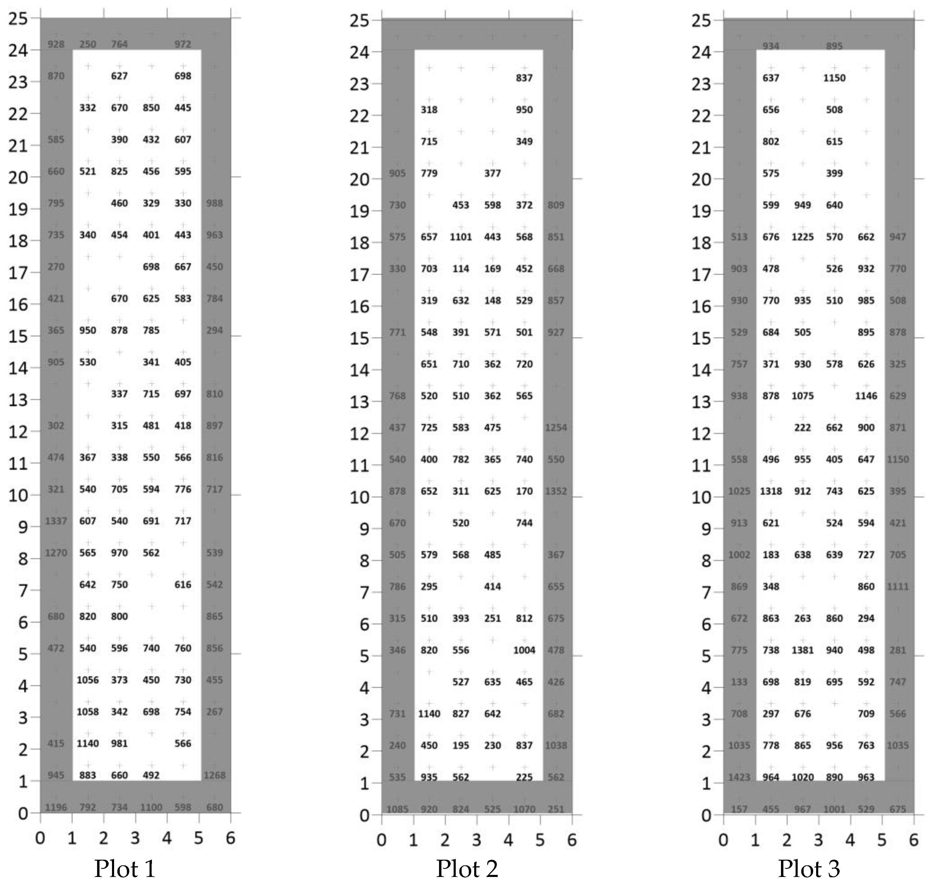
2.1. Site Description and Sampling

A maize (hybrid AGN720, Italy) crop was established in a 3 ha field area of the Aristotle University of Thessaloniki (Greece) Farm (latitude: 40°32′1.75″ N longitude: 22°59′26.98″ E) during the 2016 growing season. The seedbed was prepared according to agricultural practices applied in the area and fertilization was made with 200 and 100 kg N and P/ha, respectively. In late April (27 April 2016), the field was sown with a 4-row pneumatic sowing machine, known as Gaspardo. Weed control was achieved with the recommended field rate of the early post-emergence-applied herbicide Modett 25/28 SE (25% terbuthylazine + 28% dimethenamid-p), whereas irrigation was performed according to the requirements of the crop plants. After crop emergence, three randomly taken plots (4 m × 4.25 m) with six rows per plot were marked. The distance between the crop rows was 80 cm and that between the plants in the same row was 17 cm. Therefore, there were 25–26 plants/row, 150 plants/plot, and 450 plants in total. The distance between the three plots was 20 m. The individual plants in the three plots (Figure 1), for the purpose of the study, were considered as the units of the target statistical population from which the samples had been taken.

At the silage stage (when the kernels began to glaze) of maize (14 weeks after sowing), all plants were harvested from each subplot and the silage yield (fresh weight—FW) of each plant was recorded. The silage stage was determined by breaking the ears of maize and visually evaluating the kernels’ stage of development.

A “crop edge” of one-plant field margin (roughly 0.7 m in width) was used for each plot (Figure 2) to study its effect on data variability. Block Kriging and log₁₀ transformation were also used to estimate the mean and CV values of the original, interpolated, and log₁₀-transformed FW data for the three plots. These parameters were estimated for all harvested plants in each plot (Figure 1) and for the plants that do not include the edge (margin) ones (Figure 2). This was made to test the hypothesis that margin plants affect both variability and mean values.

2.2. Theoretical Background

2.2.1. The Use of Log Transformation in Achieving Normality and Reducing Variability in Data

Observed data from experiments and research projects are often so skewed that standard statistical analysis provides unsafe or even invalid results. Log transformation is widely used to transform skewed data to approximately conform to normality as it is easily applied and has a great effective reduction in data variability [32]. However, if the original data used do not follow a log-normal distribution, then the log transformation method does not reduce the skewness of the distribution, eliciting the risk that transformation can lead to different mean values, while making the distribution even more skewed than the original. Moreover, in contrast to popular belief, log transformation cannot always reduce the variability of data, and even in the case where this process can reduce variability, mean values must be taken into consideration.

The mean of log-transformed data $(\log y_i),\left({\widehat{\mu }}_{LT}\right)=\left(\frac{1}{n}\right)\times {{\displaystyle \sum }}_{i=1}^n\log y_i$ is used to estimate the population mean of the original data by applying the anti-log function to obtain $\exp \left({\widehat{\mu }}_{LT}\right)$. If $y_i$ follows a log-normal distribution (μ, σ²), then the mean of $y_i$ is given by $E\left(y_i \right)=\exp \left(\mu +\frac{{\sigma }^2}{2}\right)$ [32]. Afterward, if we apply log transformation to $y_i$, the transformed $\log y_i$ will follow a normal distribution with the μ mean. Therefore, $\widehat{\mu }=\exp \left({\widehat{\mu }}_{LT}\right)$ is an estimate of exp(μ). However, the mean of the original data $y_i$ is $\exp \left(\mu +\frac{{\sigma }^2}{2}\right)$, and not exp(μ). This means that even in the best situation, estimating the mean of the original $y_i$ using the anti-log of the sample mean of the log-transformed data can lead to unsafe or even invalid and misleading estimates of the population mean of the original data. Since log transformation is frequently used in agricultural research, it is worth investigating whether the potential issues with its application extend to agricultural data derived from experiments. Thus, it is pertinent to examine or confirm if log transformation raises similar concerns in agricultural research and whether alternative methods can provide more reliable outcomes.

2.2.2. Using Kriging Interpolation to Estimate Missing Data and Reduce Outliers

The idea of ‘optimal linear prediction’ was initially attributed to Kolmogorov (1941) and finally presented by Krige in 1951. Ordinary kriging, the most frequently used interpolation kriging type, has been used to effectively deliver visually appealing yield maps [19,20,21,22] for corn grain and silage yield data [23]. This interpolation method delivers accurate predictions in a selected area by producing new accurate grids of data (with the new estimates). Kriging differs from other interpolation methods in the fact that it uses the spatial correlation between sampled values to interpolate (estimate) all values in the spatial field. The estimation of values is based on the spatial arrangement of empirical observations, rather than on a presumed model of spatial distribution.

One of the advantages of applying interpolation in agricultural experimental data is that missing values (i.e., plants that did not emerge) can be estimated using the best linear unbiased prediction (BLUP). Thus, in case the data set is suffering from missing values, ordinary kriging can be used to estimate values in non-sampling locations. Moreover, depending on the parameters used, interpolation can be used as an “approximate method” in such a way as to smoothly reduce the effect of existing extreme upper or lower values (outliers). Stationarity (that the mean and variance of the values is constant across the spatial field) and isotropy (uniformity in all directions) assumptions, in the case of using hybrid plant data in ordinary kriging interpolation, can be easily anticipated.

Kriging achieves the best linear unbiased prediction. We can predict the value Z(x₀) of the random function Z = Z(x) at any arbitrary location of interest x₀, based on the nearest measured observations z(x_i) of Z(x) at the sample points x_i. In fact, kriging uses a weighted average value of the nearest observations based on the variogram or covariance function of Z(x). As prediction variance is minimized, the accuracy of the linear predictor increases, and finally the best linear prediction is achieved [5,8,33].

The estimation of the unsampled value Z at location x₀ is given by the following equation (Equation (1)):

$$Z_w^{*}\left(x_0\right):={\displaystyle \sum }_{i=1}^n{w}_{i}Z\left(x_i\right)$$

(1)

where the weights $w_i$ denotes kriging weights at location $x_i$ with the sampled value Z(x_i) and they are determined such that $Z_w^{*}\left(x_0\right)$ is an unbiased estimate of $Z_w\left(x_0\right)$ and Z(x_i) denotes sampled values in the estimation region used for the calculation of values at locations x₀, which are both demonstrated in the following equation (Equation (2)):

$${\sigma }_{{\rm E}}^2=Var\left\{Z_w^{*}\left(x_0\right)-Z\left(x_0\right)\right\}$$

(2)

In the case of kriging used as a smooth interpolator (Block Kriging), the aim is to estimate the average value of a “block” centered on the grid nodes (with the size and shape of a grid cell), as defined during the interpolation process. As a result, Block Kriging compared to Point Kriging can provide estimates and smooth interpolated results using neighboring cells to estimate a value of each block [12].

2.3. Data Analysis

The descriptive statistics of the original, log₁₀-transformed, and interpolated FW data were determined using IBM SPSS v.28 software and MS Excel. Spatial interpolation (Point Kriging and Block Kriging) was performed using Surfer for Windows. The main descriptive statistics [mean, standard deviation (SD), minimum (min), maximum (max), skewness, kurtosis, and coefficient of variation (CV)] were calculated separately for each plot to compare the crop response between the three plots. Regarding skewness, this was examined to show data scattering and flatness. Descriptive statistics were calculated for all data and for those that did not include the margin plants.

The log₁₀-transformed and interpolated FW data were initially calculated and then used to estimate the CV and mean values to be compared with the respective values for two sampling scenarios: (a) all harvested plant data and (b) all excluding data from margin plants. Block Kriging was used as smooth interpolator [12] to estimate missing values and to smooth existing extreme values, while Point Kriging was used as a reference (with results/estimates closer to the original data). It must be mentioned that Block Kriging was used to estimate the average value of rectangular blocks (areas with data) centered on the grid nodes (where the size and shape of each block being the same of a grid cell) of a given grid, while Point Kriging was used as an exact interpolator that estimates the values at the grid nodes that can provide estimated values as close as possible to the real data.

3. Results

3.1. Descriptive Statistics of the Original, Log₁₀-Trarnsformed, and Interpolated Kriging Maize Fresh Weight Data

Τhe removal of margin plants reduced the number of the harvested plants in the three plots from the initial 111–119 to 72–75, while the respective calculated means were reduced from 598–730 to 548–720 (

Table 1. Descriptive statistics of all original maize fresh weight data (g per plant) recorded in the three plots and those excluding the margin ones.

Plot	Data Used	n	Min	Max	Mean	CV (%) +	SD ++	Variance	Skewness	Kurtosis
1	All harvested	119	250	1337	649	36.9	239.5	57,351.3	0.5	0.0
	No margin	75	315	1140	611	32.2	196.5	38,629.2	0.5	−0.2
2	All harvested	111	114	1352	598	41.6	248.7	61,830.4	0.5	0.1
	No margin	72	114	1140	548	41.0	224.8	50,536.6	0.3	0.0
3	All harvested	116	133	1352	730	35.6	259.8	67,495.7	0.0	−0.1
	No margin	75	183	1381	720	34.5	248.3	61,664.5	0.2	0.1

⁺ CV: coefficient of variance, ⁺⁺ SD: standard deviation.

). The estimated CV values for all harvested plants in the three plots ranged from 35.6% to 41.6%, while the respective CVs for the plants without the margin ones ranged from 32.2% to 41.0%. In general, the second field plot produced the lower mean value and the higher CV value as compared to the other two plots.

The CV values of all log₁₀-transformed harvested plant data in the three plots ranged from 6.0% to 7.4%, while the back-log₁₀-transformed means ranged from 542 to 674 (

Table 2. Descriptive statistics of all log₁₀-transformed maize fresh weight data (g per plant) recorded in the three plots and those excluding the margin ones.

Plot	Data Used	n	Min	Max	Mean *	CV (%) +	SD ++	Variance	Skewness	Kurtosis
1	All harvested	119	2.4	3.1	605	6.0	0.2	0.028	−0.3	−0.6
	No margin	75	2.5	3.1	580	5.2	0.1	0.020	−0.2	−0.7
2	All harvested	111	2.1	3.1	542	7.5	0.2	0.042	−0.8	0.8
	No margin	72	2.1	3.1	496	7.7	0.2	0.043	−0.9	0.9
3	All harvested	116	2.1	3.2	674	6.7	0.2	0.036	−1.3	2.3
	No margin	75	2.3	3.1	673	6.1	0.2	0.030	−1.0	1.4

* Back log₁₀-transformed means, ⁺ CV: coefficient of variance, ⁺⁺ SD: standard deviation.

). Regarding the harvested plants without the margin ones, the CV and mean values ranged from 5.2% to 7.7% and from 496 to 673, respectively. As the original data, the second field plot produced the lower mean value and the higher CV value as compared to the other two plots.

The CV values of Point Kriging interpolated all harvested plant data in the three plots ranged from 31.4% to 35.8%, while the calculated means ranged from 600 to 728 (

Table 3. Descriptive statistics for the Point Kriging interpolated maize fresh weight data (g per plant) recorded in the three plots and those excluding the margin ones.

Plot	Kriging Type	Data Used	n	Min	Max	Mean	CV (%) +	SD ++	Variance	Skewness	Kurtosis
1	Point Kriging	All harvested	150	250	1337	646	33.4	215.5	46,447.5	0.6	0.6
		No margin	92	315	1140	611	29.5	180.3	32,518.2	0.5	0.3
2	Point Kriging	All harvested	150	114	1352	600	35.8	214.6	46,047.3	0.5	1.1
		No margin	92	114	1140	558	35.9	200.4	40,160.6	0.2	0.6
3	Point Kriging	All harvested	150	133	1423	728	31.4	228.8	52,332.0	0.1	0.8
		No margin	92	183	1381	720	31.2	224.5	50,418.2	0.2	0.8

⁺ CV: coefficient of variance, ⁺⁺ SD: standard deviation.

). Regarding the harvested plants without the margin ones, the CV and mean values ranged from 29.5% to 35.9% and from 558 to 720, respectively. As the original and log₁₀-transformed data, the second field plot produced a lower mean value and a higher CV value as compared to the other two plots.

The CV values of all harvested plant Block Kriging interpolated data in the three plots ranged from 14.5% to 19.9%, while the calculated means ranged from 600 to 728 (

Table 4. Descriptive statistics for the Block Kriging interpolated maize fresh weight data (g per plant) recorded in the three plots and those excluding the margin plants.

Plot	Kriging Type	Data Used	n	Min	Max	Mean	CV (%) +	SD ++	Variance	Skewness	Kurtosis
1	Block Kriging	All harvested	150	404	1033	646	19.9	128.3	16,468.4	0.5	0.4
		No margin	92	404	948	621	18.0	112.0	12,545.9	0.3	0.2
2	Block Kriging	All harvested	150	323	950	600	18.1	108.6	11,799.2	0.4	0.7
		No margin	92	323	849	571	17.3	99.0	9804.2	0.2	0.4
3	Block Kriging	All harvested	150	452	1036	728	14.5	105.3	11,085.3	0.1	0.4
		No margin	92	495	1015	723	14.3	103.3	10,662.48	0.4	0.3

⁺ CV: coefficient of variance, ⁺⁺ SD: standard deviation.

). Concerning the harvested plants without the margin ones, the CV and mean values ranged from 14.3% to 18.0% and from 571 to 723, respectively. Again, the second field plot produced the lower mean values as compared to the other two plots, but its CV values were higher than those of the third plot.

The above findings (Table 1, Table 2, Table 3 and Table 4) indicate that log₁₀ transformation resulted in a greater reduction in the data variability (CV) of all harvested original FW maize plant data and those excluding margin plants in the three plots as compared with that of point and Block Kriging. However, the Block Kriging CVs were reduced more than the respective ones of Point Kriging. The back-log₁₀-transformed means of all harvested FW plant data were reduced by 6.8–9.4% as compared to the original data, while the respective reduction in the plants (excluding margin ones) was 1.3–8.3%. The Point Kriging means for all harvested plants and for those excluding the margin ones were reduced by 0.1–0.5% as compared to the original data, while the respective reduction in Block Kriging means for all harvested plant data was 0.3–0.4%. By contrast, the estimated means of the harvested plants excluding margin ones were increased by 0.4–4.3% as compared to the original data. In response to the first scientific question raised, it can be concluded that the harvested maize plants grown in the border (margin) rows did not significantly affect the data variability and the mean values of plants grown in the central rows of the experimental field plots. Additionally, Block Kriging achieved a reduction in data variability, keeping the means as close as possible to the original data (only up to 0.4%) compared to log₁₀ transformation data that altered the means (up to 10%).

3.2. Box Plots of the Original and Interpolated Kriging Maize Fresh Weight Data

The box plots, which were constructed from the minimum value, the maximum value, the first quartile, the median, and the third quartile of the data, revealed that the decreasing order of the locality, spread, and skewness groups of numerical data through their quartile was as follows: “all original harvested plants in the three field plots” > “original plants without the margin ones” > “interpolated with Point Kriging” > “interpolated with Block Kriging” (Figure 3).

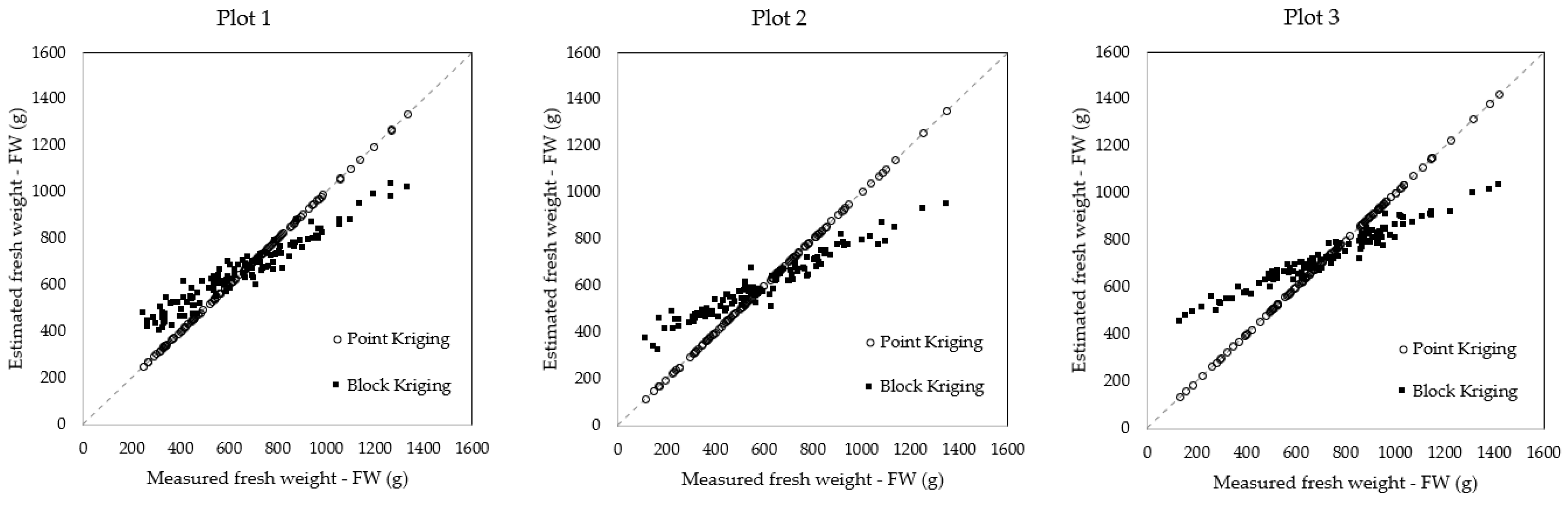
3.3. Diagrammatic Presentation of the Original, Point, and Block Kriging Data

A visual representation of the original fresh weight (FW) data in the three field plots, along with the estimated values obtained through point and Block Kriging methods, reveals that both techniques successfully estimated the missing values. However, it is apparent from the diagram that the Block Kriging method also effectively smoothed out extreme values (higher and lower) in the original data, while Point Kriging delivered estimates very close to the original data. This smoothing effect of Block Kriging can be observed in Figure 4 for all three plots.

Although Point Kriging, as an exact interpolator, can achieve more precise estimations, in this case, the application of interpolation was not aimed at getting as close as possible to the original data. Rather, the objective was to smoothen out lower and higher values while keeping the means almost constant.

As shown in Figure 5, a comparison between measured and estimated fresh weight data graphs reveals that Block Kriging produced a smoother outcome than Point Kriging and this smoothing effect mainly impacted the lower and higher values (which may be considered as not being representative from the agronomic perspective). In addition, the scatter plot for Point Kriging reveals that all estimated values align precisely with the reference line, presenting the expected result of an exact interpolator. On the other hand, the scatter plot for Block Kriging shows that lower and higher values were smoothed out, while values near the mean were only slightly affected. This representation highlights how, despite modifying several data points, the mean remains constant and almost identical to the mean of the original data.

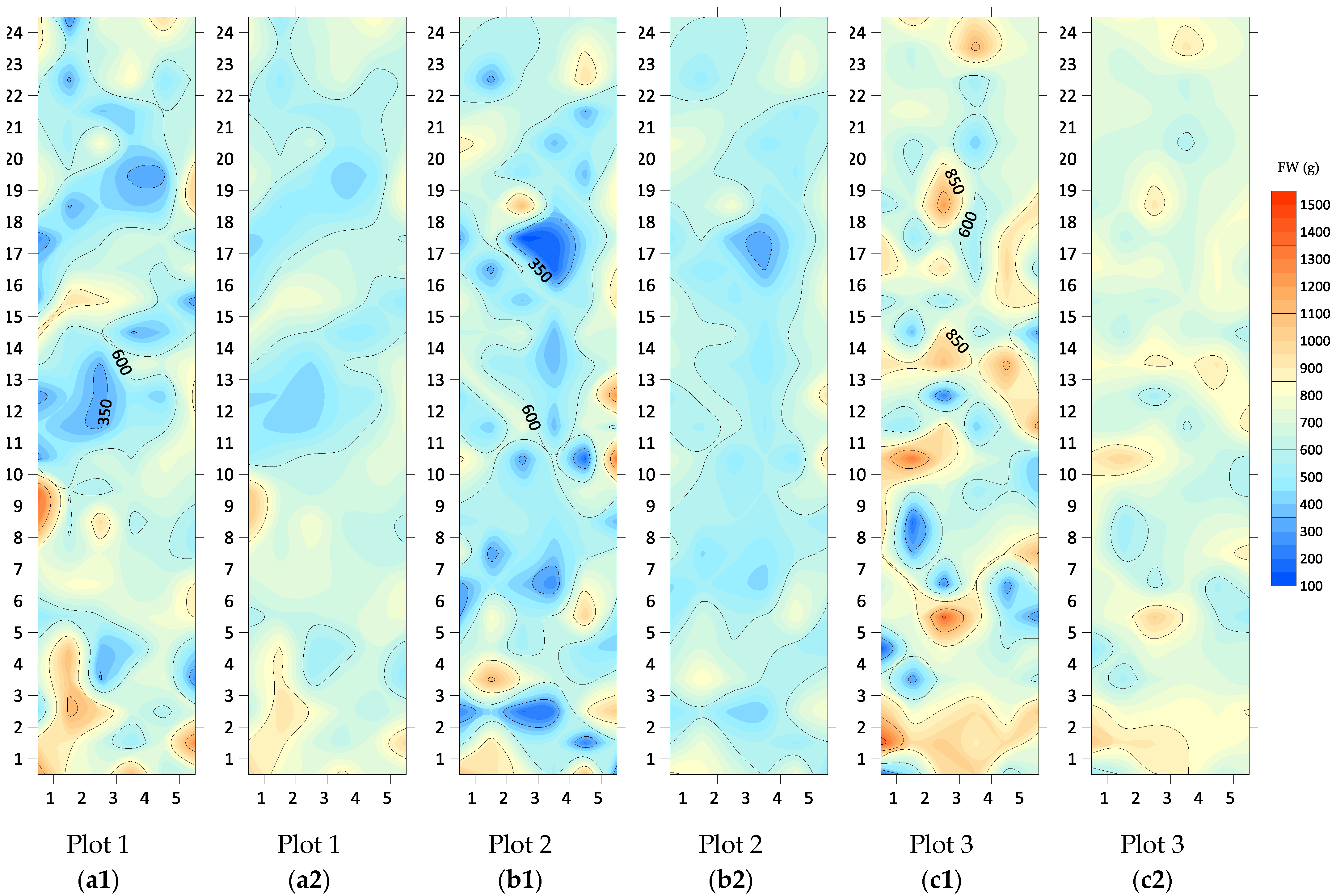
3.4. Contour Maps of the Point and Block Interpolation Grids

In all plots, the same hybrid was utilized, and consistent agronomical practices were implemented across the three plots situated in the same region. Consequently, the observed variability in yield data (fresh weight) can likely be attributed to factors such as environmental conditions and soil characteristics, rather than the hybrid itself. Hence, it is inferable that interpolation can be effectively applied to the original point data within each plot, treating the yield as a continuous variable. In this context, contour maps were constructed with “Surfer for Windows” to provide a better visual view of the point and block interpolation grids (Figure 6). The purpose of displaying the contour maps is to illustrate the spatial discrepancies between the results obtained from point and Block Kriging, with a specific focus on the smoothing effect provided by Block Kriging. Moreover, the contour maps provide a visual representation of the estimated values, allowing for a more detailed examination of the spatial distribution of data. In particular, the contour maps of Block Kriging (a2, b2, and c2) had less brown/dark blue color areas corresponding to low/high (extreme) values than the respective areas of Point Kriging (a1, b1, and c1) because of the smoothing effect on data. By comparing the contour maps generated from both interpolation methods, it becomes apparent that Block Kriging smooths out the extreme values, resulting in a more gradual transition between areas with high and low values. This smoothing effect is especially evident in areas where there were missing values or extreme values in the original data. Therefore, in this case, the contour maps serve as a valuable tool in understanding the differences between point and Block Kriging, and the advantages of using Block Kriging to address missing values and reduce variability in agricultural data.

3.5. Fitted Variogram Variables for Point and Block Kriging

The most suitable fitted model for both point and Block Kriging interpolated maize data in the three field plots was the exponential (

Table 5. Geostatistical variables of the best-fitted variogram models for both point and Block Kriging data recorded in the three field plots.

Kriging Type	Plot	n	Variogram	Nugget	Sill	Range	R2	RSS	RMSE
Point Kriging	1	150	Exponential	0	53,470	0.96	0.99	9.5 × 10−12	2.5 × 10−7
Block Kriging	1	150	Exponential	0	53,510	0.97	0.93	14.5 × 105	98.5
Point Kriging	2	150	Exponential	0	60,600	0.70	0.99	6.3 × 10−12	2.04 × 10−7
Block Kriging	2	150	Exponential	0	60,270	0.72	0.94	1.9 × 105	113.5
Point Kriging	3	150	Exponential	0	68,000	0.53	0.99	8.2 × 10−12	2.34 × 10−7
Block Kriging	3	150	Exponential	0	68,000	0.62	0.96	24.7 × 105	128.4

where R² = coefficient of determination; RSS = residual sum of squares, RMSE = root mean square error. The bold print shows the highest values per plot.

) and it was selected after comparing the performance of other models based on their R² values and root mean square errors (RMSEs). Table 5 presents the results of Point Kriging and Block Kriging for the three different plots, providing information about the variogram model parameters (variogram type, nugget, sill, and range); goodness-of-fit measures; and the following accuracy measures: (a) residual sum of squares (RSS), which measures the sum of squared differences between the observed values and the predicted values from the kriging model (RSS), and (b) root mean square error (RMSE), which is the standard deviation of residuals (differences between observed and predicted values). Overall, both Point Kriging and Block Kriging have high R² values (R² represents the coefficient of determination, which measures the goodness-of-fit of the variogram model to the data) across all plots, indicating a very good fit of variogram models to the fresh weight data.

4. Discussion

This study was conducted to investigate and assess the performance of log₁₀ transformation and Block Kriging interpolation on reducing maize fresh weight data variability. The log₁₀ transformation method was tested because is the most widely used method in agricultural, biomedical, and psychosocial research to stabilize and reduce variability of data and ensure more close conformity to the normal distribution or, in general, to asymmetric distribution [2,11,12]. On the other hand, the kriging interpolation method was selected and compared with the log₁₀ transformation method because several previous studies have indicated its importance in reducing data variability and adequately estimating missing and mean values [13,20,22,31].

The significant reduction in variability (CV) due to log₁₀ transformation, as compared to the respective CVs of all original harvested FW plant data and those excluding margin plants in all plots, justifies its popular use in agricultural research for reducing data variability. However, the fact that back-transformed estimated means after log₁₀ transformation were reduced as compared with the original ones makes the interpretation of results meaningless, since the adjusted crop yield means of the expected real values were underestimated on the original scale [2]. Several studies [2,11] have indicated that log₁₀ transformation has been misused, even by statisticians, leading to incorrect interpretations of experimental results [2,11]. Therefore, it is suggested that, if log₁₀ transformation must be used, the researcher must be mindful about its limitations, particularly when interpreting the relevance of transformed data analysis for the hypothesis of interest regarding original data.

The greater reduction in Block Kriging CVs as compared to those of Point Kriging suggests its possible use in agricultural research. In addition, the lower change in the estimated Block Kriging mean values as compared to the back-log₁₀-transformed values strongly suggests that Block Kriging, in addition to the adequate estimation of missing values at non-sampled locations (places where plants did not emerge), can effectively replace the most commonly used statistical method of log₁₀ transformation since it can offer both a reduction in data variability and a more precise crop yield estimate. It is worth mentioning that the above findings were confirmed by descriptive statistics of the original; log₁₀-trarnsformed and interpolated kriging maize fresh weight data; box plots of the original and interpolated kriging maize fresh weight data; a diagrammatic presentation of the original, point, and Block Kriging data; the contour maps of point and block interpolation grids; and fitted variogram variables for point and Block Kriging data.

Achieving better estimates for crop production via Block Kriging is crucial; for example, the 10% less estimated maize crop yield (using log₁₀ transformation so far), as compared to the original means, reduces the total maize yield by up to 2 tn/ha (with an average maize yield of 12–18 tn/ha) and estimates non-existent economic loss for maize growers. Therefore, it can be deduced that Block Kriging must be favored over log₁₀ transformation to address missing values and reduce data variability, and as a result to provide more safe and accurate crop metrics.

5. Conclusions

The findings of this study allow the following conclusions to be drawn:

• Log₁₀-transformation was found appropriate at the analysis stage of maize crop yield data as provides a notable reduction in data variability (CV values), but it failed to estimate means leading to non-existent economic loss for the producers.
• The Block Kriging interpolation method was found to adequately replace the commonly used the statistical method of log₁₀ transformation so far as it managed to reduce data variability without altering the means, leading to more precise estimates of crop yield. A summary of the highlighted advantages of Block Kriging interpolation versus log₁₀ transformation showed that this method can successfully (a) estimate and fill in missing values, (b) smooth unrepresentative or extreme values (usually present in agricultural data), (c) adjust the estimated values to account for the spatial correlation of experimental units with respect to the measured characteristics, (d) reduce the data variability without altering the estimated mean values of the measured characteristics, and (e) improve the overall quality of the data.

Therefore, Block Kriging can efficiently replace the log₁₀ transformation method, which provides a significantly reduction in CV values, but also leads to significant erroneous estimates for larger areas in most cases. Block Kriging can effectively address the issue of missing values and reduce variability in maize field yield data, while keeping the means almost constant, providing more accurate crop metrics to assess field productivity.

References

1. Nogueira Martins, R.; Ferreira Lima Dos Santos, F.; de Moura Araújo, G.; de Arruda Viana, L.; Fim Rosas, J.T. Accuracy Assessments of Stochastic and Deterministic Interpolation Methods in Estimating Soil Attributes Spatial Variability. Commun. Soil Sci. Plant Anal. 2019, 50, 2570–2578. [Google Scholar] [CrossRef]
2. Piepho, H.P. Data Transformation in Statistical Analysis of Field Trials with Changing Treatment Variance. Agron. J. 2009, 101, 865–869. [Google Scholar] [CrossRef]
3. Kosmowski, F.; Chamberlin, J.; Ayalew, H.; Sida, T.; Abay, K.; Craufurd, P. How Accurate Are Yield Estimates from Crop Cuts? Evidence from Smallholder Maize Farms in Ethiopia. Food Policy 2021, 102, 102122. [Google Scholar] [CrossRef] [PubMed]
4. Lobell, D.B.; Azzari, G.; Burke, M.; Gourlay, S.; Jin, Z.; Kilic, T.; Murray, S. Eyes in the Sky, Boots on the Ground: Assessing Satellite- and Ground-Based Approaches to Crop Yield Measurement and Analysis. Am. J. Agric. Econ. 2020, 102, 202–219. [Google Scholar] [CrossRef]
5. Norman, J.M.; Becker, F. Terminology in Thermal Infrared Remote Sensing of Natural Surfaces. Agric. For. Meteorol. 1995, 77, 153–166. [Google Scholar] [CrossRef]
6. Wahab, I. In-Season Plot Area Loss and Implications for Yield Estimation in Smallholder Rainfed Farming Systems at the Village Level in Sub-Saharan Africa. GeoJournal 2020, 85, 1553–1572. [Google Scholar] [CrossRef]
7. Abay, K.A.; Abate, G.T.; Barrett, C.B.; Bernard, T. Correlated Non-Classical Measurement Errors, ‘Second Best’ Policy Inference, and the Inverse Size-Productivity Relationship in Agriculture. J. Dev. Econ. 2019, 139, 171–184. [Google Scholar] [CrossRef]
8. Poate, D. A Review of Methods for Measuring Crop Production from Smallholder Producers. Exp. Agric. 1988, 24, 1–14. [Google Scholar] [CrossRef]
9. Ndakidemi, B.J.; Mbega, E.R.; Ndakidemi, P.A.; Belmain, S.R.; Arnold, S.E.J.; Woolley, V.C.; Stevenson, P.C. Field Margin Plants Support Natural Enemies in Sub-Saharan Africa Smallholder Common Bean Farming Systems. Plants 2022, 11, 898. [Google Scholar] [CrossRef]
10. Marshall, E.J.P.; Moonen, A.C. Field Margins in Northern Europe: Their Functions and Interactions with Agriculture. Agric. Ecosyst. Environ. 2002, 89, 5–21. [Google Scholar] [CrossRef]
11. Mante, J.; Gerowitt, B. Learning from Farmers’ Needs: Identifying Obstacles to the Successful Implementation of Field Margin Measures in Intensive Arable Regions. Landsc. Urban Plan. 2009, 93, 229–237. [Google Scholar] [CrossRef]
12. Feng, C.; Wang, H.; Lu, N.; Chen, T.; He, H.; Lu, Y.; Tu, X.M. Log-Transformation and Its Implications for Data Analysis. Shanghai Arch. Psychiatry 2014, 26, 105–109. [Google Scholar] [CrossRef]
13. Cressie, N. Block Kriging for Lognormal Spatial Processes. Math. Geol. 2006, 38, 413–443. [Google Scholar] [CrossRef]
14. Taleb, I.; Serhani, M.A.; Bouhaddioui, C.; Dssouli, R. Big Data Quality Framework: A Holistic Approach to Continuous Quality Management. J. Big Data 2021, 8, 76. [Google Scholar] [CrossRef]
15. Desiere, S.; Jolliffe, D. Land Productivity and Plot Size: Is Measurement Error Driving the Inverse Relationship? J. Dev. Econ. 2018, 130, 84–98. [Google Scholar] [CrossRef]
16. Kim, T.; Ko, W.; Kim, J. Analysis and Impact Evaluation of Missing Data Imputation in Day-Ahead PV Generation Forecasting. Appl. Sci. 2019, 9, 204. [Google Scholar] [CrossRef]
17. Piepho, H.P.; Möhring, J.; Williams, E.R. Why Randomize Agricultural Experiments? J. Agron. Crop Sci. 2013, 199, 374–383. [Google Scholar] [CrossRef]
18. Fermont Volcafe, A.; Benson, T. Estimating Yield of Food Crops Grown by Smallholder Farmers: A Review in the Uganda Context Evolution of Farming Systems in Africa View Project; International Food Policy Research Institute: Washington, DC, USA, 2011. [Google Scholar]
19. Hancock, G.R. The Impact of Different Gridding Methods on Catchment Geomorphology and Soil Erosion over Long Timescales Using a Landscape Evolution Model. Earth Surf. Process Landf. 2006, 31, 1035–1050. [Google Scholar] [CrossRef]
20. Tziachris, P.; Metaxa, E.; Papadopoulos, F.; Papadopoulou, M. Spatial Modelling and Prediction Assessment of Soil Iron Using Kriging Interpolation with PH as Auxiliary Information. ISPRS Int. J. Geoinf. 2017, 6, 283. [Google Scholar] [CrossRef]
21. Ismail, H.Y.; Fayyad, S.; Ahmad, M.N.; Leahy, J.J.; Naushad, M.; Walker, G.M.; Albadarin, A.B.; Kwapinski, W. Modelling of Yields in Torrefaction of Olive Stones Using Artificial Intelligence Coupled with Kriging Interpolation. J. Clean. Prod. 2021, 326, 129020. [Google Scholar] [CrossRef]
22. Wiens, D.P.; Zhou, J. Robust Estimators and Designs for Field Experiments. J. Stat. Plan. Inference 2008, 138, 93–104. [Google Scholar] [CrossRef]
23. Cho, J.B.; Guinness, J.; Kharel, T.P.; Sunoj, S.; Kharel, D.; Oware, E.K.; van Aardt, J.; Ketterings, Q.M. Spatial Estimation Methods for Mapping Corn Silage and Grain Yield Monitor Data. Precis. Agric. 2021, 22, 1501–1520. [Google Scholar] [CrossRef]
24. Bowman, D.T. Crop Ecology, Production, & Management: Plot Configuration in Corn Yield Trials. Crop Sci. 1989, 29, 1202–1206. [Google Scholar] [CrossRef]
25. Buttafuoco, G.; Castrignanò, A.; Cucci, G.; Lacolla, G.; Lucà, F. Geostatistical Modelling of Within-Field Soil and Yield Variability for Management Zones Delineation: A Case Study in a Durum Wheat Field. Precis. Agric. 2017, 18, 37–58. [Google Scholar] [CrossRef]
26. Maldaner, L.F.; Molin, J.P. Data Processing within Rows for Sugarcane Yield Mapping. Sci. Agric. 2020, 77, e20180391. [Google Scholar] [CrossRef]
27. Betzek, N.M.; de Souza, E.G.; Bazzi, C.L.; Schenatto, K.; Gavioli, A.; Magalhães, P.S.G. Computational Routines for the Automatic Selection of the Best Parameters Used by Interpolation Methods to Create Thematic Maps. Comput. Electron. Agric. 2019, 157, 49–62. [Google Scholar] [CrossRef]
28. McKinion, J.M.; Willers, J.L.; Jenkins, J.N. Spatial Analyses to Evaluate Multi-Crop Yield Stability for a Field. Comput. Electron. Agric. 2010, 70, 187–198. [Google Scholar] [CrossRef]
29. Allakonon, M.G.B.; Zakari, S.; Tovihoudji, P.G.; Fatondji, A.S.; Akponikpè, P.B.I. Grain Yield, Actual Evapotranspiration and Water Productivity Responses of Maize Crop to Deficit Irrigation: A Global Meta-Analysis. Agric. Water Manag. 2022, 270, 107746. [Google Scholar] [CrossRef]
30. Yan, P.; Lin, K.; Wang, Y.; Zheng, Y.; Gao, X.; Tu, X.; Bai, C. Spatial Interpolation of Red Bed Soil Moisture in Nanxiong Basin, South China. J. Contam. Hydrol. 2021, 242, 103860. [Google Scholar] [CrossRef]
31. Řezník, T.; Pavelka, T.; Herman, L.; Leitgeb, Š.; Lukas, V.; Širůček, P. Deployment and Verifications of the Spatial Filtering of Data Measured by Field Harvesters and Methods of Their Interpolation: Czech Cereal Fields between 2014 and 2018. Sensors 2019, 19, 4879. [Google Scholar] [CrossRef] [PubMed]
32. Koutsos, T.M.; Menexes, G.C.; Eleftherohorinos, I.G. The Use of Spatial Interpolation to Improve the Quality of Corn Silage Data in Case of Presence of Extreme or Missing Values. ISPRS Int. J. Geoinf. 2022, 11, 153. [Google Scholar] [CrossRef]
33. Zimmerman, D.L.; Zimmerman, M.B. A Comparison of Spatial Semivariogram Estimators and Corresponding Ordinary Kriging Predictors. Technometrics 1991, 33, 77–91. [Google Scholar] [CrossRef]
Figure 1. Schematic presentation of the plants harvested and their fresh weight (FW) in the three randomly taken plots (plot 1: 119 plants; plot 2: 111 plants; plot 3: 116 plants). Values represent original FW values of harvested plants (+), and empty spots (without numbers) represent locations where plants did not emerge (missing values).
Agronomy 13 01685 g001
Figure 2. Schematic presentation of the original FW plant values in each of the three plots (Plots 1–3) without the edge (margin) plants. Dark areas represent the “margin” in each one of the three randomly taken plots. Empty spots represent locations where plants did not emerge (missing values).
Agronomy 13 01685 g002
Figure 3. Box plots of all original and those excluding (“No margin”) the margin maize fresh weight (FW) data recorded in the three plots (Plots 1–3), along with data interpolated using point and Block Kriging methods.
Agronomy 13 01685 g003
Figure 4. Schematic cross-sections in the three field plots (Plot 1–3) of all original measurements (points) and the corresponding estimated values using Point Kriging (circles) and Block Kriging (squares). Capital letters (A–G) represent the starting and ending points of each row (section)/plot.
Agronomy 13 01685 g004
Figure 5. Original fresh weight (FW) vs. estimated data using point and Block Kriging in the three field plots (Plots 1–3).
Agronomy 13 01685 g005
Figure 6. Contour maps for interpolated fresh weight (FW) data in the three plots, where (a1,b1,c1) correspond to Point Kriging and (a2,b2,c2) to Block Kriging.
Agronomy 13 01685 g006