Abstract
Physically-based parameter estimations are essential to improve the simulation performance of a hydrologic model and to produce physically reasonable parameters with spatial consistency. This study proposed a parameter derivation strategy to improve the Sacramento Soil Moisture Accounting (SAC-SMA) model simulation performance based on the publicly accessible Harmonized World Soil Database (HWSD). The HWSD soil properties were used to estimate the soil moisture characteristics, and the HWSD soil texture classifications and International Geosphere-Biosphere Programme (IGBP) land cover types were used to identify the Soil Conservation Service (SCS) runoff curve number (CN). After the soil moisture characteristics and CNs were identified, the major parameters of the SAC-SMA model were derived. The simulation results were evaluated using the Nash efficiency coefficient (NSEC), and Free Search (FS) algorithm was used to further adjust and calibrate the parameters. Compared with the simulation accuracy (NSEC = 0.66~0.88) and parameter transferability (NSEC = 0.22~0.83) obtained for the SAC-SMA model using directly calibrated parameters, the HWSD data-derived parameters allowed the SAC-SMA model to achieve a similar simulation accuracy (NSEC = 0.65~0.86) and a better transferability (NSEC = 0.61~0.85).
1. Introduction
Hydrologic models are effective tools to simulate and evaluate the quantity and quality of water resources and play an important role in crop planting structure adjustment and food crop production in water shortage areas [1,2,3,4,5,6]. The successful application of any hydrologic model greatly depends on its parameterization. However, hydrologic model parameters generally cannot be readily derived from the physical characteristics of basins, which greatly hinders the application of these models in geographically discrepant regions [7,8]. Even if model parameters are related to observable physical characteristics, some calibration of the priori parameters are still required because the basin-scale heterogeneities of physical characteristics and data uncertainties can both significantly affect the estimation process [9,10]. A great deal of research has explored different hydrologic model calibration approaches [11,12,13,14], these approaches often require years of historical hydrometeorological data and are usually performed for a single basin [15,16,17]. The quality and quantity of historical data can vary significantly among different regions and even among different basins in the same region [1,7,18]. These differences can lead to nonoptimal parameter values and can produce significant and inappropriate randomness in the spatial distributions of model parameters [7,18,19,20]. Therefore, there is an urgent need to develop hydrological model calibration strategies that can derive parameters with physical and spatial consistency.
The Sacramento Soil Moisture Accounting (SAC-SMA) model is a globally widely used streamflow simulation system [21,22], including 11 major parameters and 5 minor parameters [7,18]. The Hydrology Laboratory of the National Weather Service (NWS) Office of Hydrologic Development has developed a groundbreaking approach that uses physical relationships to derive 11 major parameters of the SAC-SMA model based on the State Soil Geographic Database (STATSGO, at a scale of 1:250,000) [7,8]. Additionally, Anderson et al. [19] improved the initial parameter estimation approach by using the Soil Survey Geographic Database (SSURGO, at a scale of 1:24,000). However, STATSGO and SSURGO are only available in the United States, and there is a lack of reliable soil databases globally. Although the general parameter calibration approach can obtain the “optimal” parameter sets for the SAC-SMA model, these “optimal” parameter sets are often spatially inconsistent and physically unreasonable and are thus not suitable to be transferred to other nearby basins. Therefore, it is necessary to develop a generalized strategy to produce spatially consistent and physically realistic parameters for use in the SAC-SMA model by applying an available soil database with global coverage.
The Harmonized World Soil Database (HWSD) is a 30-arc-second database that integrates varieties of regional soil datasets [23]. The HWSD provides 17 soil physicochemical properties for topsoil (0–30 cm) and subsoil (30–100 cm), and its raster database consists of 21,600 rows and 43,200 columns; 221 million grid cells cover the global land territory. Over 16,000 different soil property units have been harmonized and integrated into HWSD. The soil database provides frequently-used soil properties worldwide and is widely used in the establishment of hydrologic model databases [24,25], identification of root burial depth [26], calculation of soil hydraulic properties [27], etc. To the best of our knowledge, however, there is a lack of studies exploring the application of HWSD datasets in deriving major parameters in the SAC-SMA model.
To overcome the above problems, we develop a SAC-SMA model parameter derivation strategy to improve the performance of a model on the simulation of the runoff process. It will benefit the application of the SAC-SMA model in the region that lacks soil properties datasets. Specifically, we address the following problems. (1) Can HWSD data be used to derive the major parameters required by the SAC-SMA model? (2) Compared to the directly calibrated parameters, how does the SAC-SMA model perform using HWSD data-derived parameters? (3) Compared to the directly calibrated parameters, is the transferability of the HWSD data-derived parameters better? Section 2 describes the parameter derivation strategy based on HWSD. The selected basins, dataset, and experiment designs are introduced in Section 3, followed by the result in Section 4, and discussion in Section 5. Finally, the conclusion is given in Section 6.
2. Methodology
Based on the approach of Koren et al. [7], once the soil moisture characteristics and the United States Soil Conservation Service (SCS) runoff curve number (CN) are estimated, the major parameters of the SAC-SMA model can be derived. In this paper, we attempt to derive these parameters using the HWSD soil properties and the International Geosphere-Biosphere Programme (IGBP) land cover types; we aim to provide a more general parameter derivation strategy while considering the physical characteristics of parameters (see Figure 1). First, the soil moisture characteristics are estimated using the sand (S), clay (C), and organic carbon (OC) contents listed in the HWSD. Second, the HWSD soil texture classifications and IGBP land cover types are used to identify the CN values. Third, a priori estimates for the major parameters of the SAC-SMA model based on the above two points. Fourth, the major and minor parameters of the SAC-SMA model are further adjusted or calibrated using a population-based optimization algorithm, namely Free Search (FS).
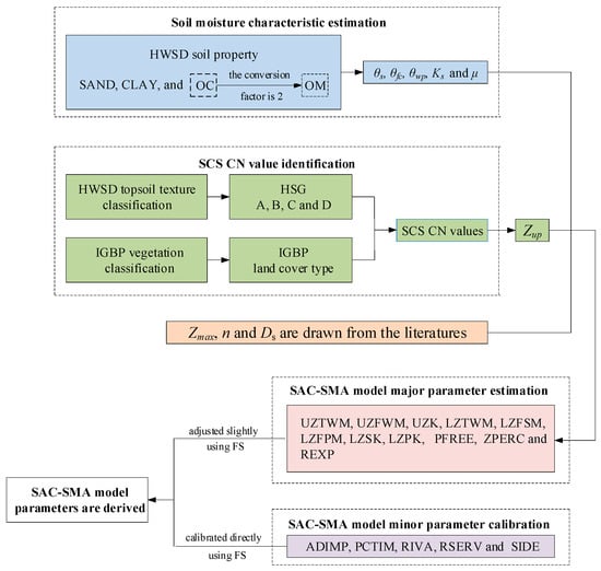
Figure 1.
Decision-making procedure of deriving SAC-SMA model parameters based on HWSD soil properties.
2.1. SAC-SMA Model Parameter and Soil Moisture Characteristic Relationships
The parameters of the SAC-SMA model are shown in Table 1. The relationship between the major parameters (highlighted in Table 1) and soil moisture characteristics is shown in Appendix A, and these soil moisture characteristics are saturated moisture content (θs), field capacity (θfc), wilting point (θwp), saturated hydraulic conductivity (Ks), and specific yield of soil (μ). To relate the major parameters to soil moisture characteristics, Koren et al. [7,8] assumed that the total depth of the upper and lower layers in the SAC-SMA model (Zmax) was equal to the total depth of the STATSGO soil profile, and the split between the upper and lower soil layers (Zup) was determined by utilizing the initial rain abstraction concept derived from the runoff curve number method.

Table 1.
SAC-SMA model parameters and their feasible ranges or default value [7,18].
To estimate the soil moisture characteristics, the percentages of sand and clay were obtained from the midpoint values of each textural class using the United States Department of Agriculture (USDA) textural triangle, and these were related to soil moisture characteristics using regression equations from Cosby et al. [28]. Experimental data reported by Clapp et al. [29] were used to estimate Ks, while an empirical relationship from Armstrong [30] was used to estimate μ. A simplified approach was used to estimate CN values based on the USDA Hydrologic Soil Group Grid (HSG) assuming ‘pasture or range land use’ under ‘fair’ hydrologic conditions for the entire region. These relationships are reported in Koren et al. [7].
However, according to Clapp et al. [29] and Cosby et al. [28], the sand, clay, and Ks can be obtained for only 11 USDA soil textures, silt soil properties are lacking and Ks is empirical. It should be noted that the HWSD classifies clay soils into heavy clay and light clay, so the HWSD has 13 USDA soil textures (see Figure 2). Therefore, it is necessary to use other approaches to estimate the 13 USDA soil moisture characteristics using the HSWD soil properties.
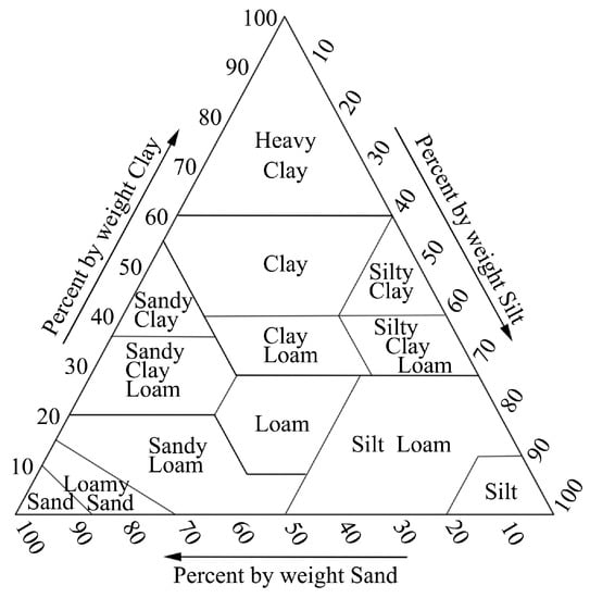
Figure 2.
USDA soil texture classifications in HWSD [23].
2.2. Estimation of Soil Moisture Characteristics Using HWSD
Saxton et al. [31] developed some equations for soil moisture characteristic estimates based on soil texture and organic matter (OM). When θwp, θfc, and θs are defined as the soil moisture contents at tensions of 1500, 33, and 0 kPa, respectively, the prediction equations are expressed as follows [31]:
where θ1500 is the 1500 kPa moisture (wilting point) at normal density, in cm3·cm−3; θ1500t is the first-solution 1500 kPa moisture, in cm3·cm−3; S, C, and OM are the sand, clay, and OM contents in the soil, respectively, in %wt.; θ33 is the 33 kPa moisture (field capacity) at normal density, in cm3·cm−3; θ33t is the first-solution 33 kPa moisture, in cm3·cm−3; θs is the 0 kPa moisture (saturated) at normal density, in cm3·cm−3; θ(s-33) is the 0–33 kPa moisture at normal density, in cm3·cm−3; and θ(s-33)t is the first-solution 0–33 kPa moisture, in cm3·cm−3.
The saturated hydraulic conductivity is related to θs and θ33 as follows:
where λ is the slope of the logarithmic tension-moisture curve.
It should be noted that a conversion factor of 1.724 has historically been used to convert the soil OC measurements into soil OM estimates [32]. Studies published since the end of the nineteenth century have consistently shown that the 1.724 conversion factor is too small for most soils. A factor of 2 was thus adopted in this research based on the assumption that soil OM contains 50% carbon [33].
In addition, μ was calculated using an empirical formula from Koren et al. [7]:
Based on Formulas (1)–(10), the S, C, and OC contents of the HWSD topsoil and subsoil layers can be used to estimate the soil moisture characteristics at a grid scale of 30 arc seconds.
2.3. CN Value Identification
Hong et al. [34] reported an attempt to derive a global CN map using satellite remote sensing and geospatial data and developed an approach for estimating CN values using a function of the hydrologic soil group (HSG), land cover type, and hydrologic conditions. In the research of Hong et al. [34] and Zeng et al. [35], global land cover data derived from the Moderate Resolution Imaging Spectroradiometer (MODIS) were used as a surrogate for land cover/use types, and the 17 land cover types were identified in the IGBP vegetation classification scheme.
When the topsoil and subsoil soil moisture characteristics of the HWSD are used to replace the upper and lower soil moisture characteristics of the SAC model, the upper-layer HSG of the SAC-SMA model can be identified according to the USDA texture of the HWSD topsoil (see Table 2), and the CN values can then be estimated using the HSGs, IGBP land cover types, and hydrologic conditions (see Table 3).
Table 2.
Hydrologic soil groups derived from soil properties [34,35].
Table 3.
CN values derived from the IGBP land cover types and hydrologic soil groups [34,35,36].
After the CN values are identified, Zup can be calculated using formula A12. At this point, the major parameters of the SAC-SMA model can be derived using Zup, Zmax, and the soil moisture characteristics of the HWSD topsoil and subsoil layers. In the study of Koren et al. [7], 25 percent of bounds from soil-derived parameters were used to adjust the soil-derived parameters. Referring to this method, these priori major parameters will be adjusted slightly in our study, and the FS was used in the automatic adjustment process. FS is an optimization algorithm based on swarm intelligence, and a detailed description of FS can be found in Penev et al. [37]; through testing, this algorithm has been shown to be efficient in finding the global optimal parameters of hydrologic models [22,38].
3. Data and Experiments
The proposed strategy was applied to a real-world study in which runoff simulations of several watersheds in the Hulan River basin in northeast China were obtained. Rainfall-runoff simulations were generated in a lumped mode assuming that the input data and model parameters were uniform over each analyzed watershed. According to the SAC-SMA model simulation accuracy, the results of the application of the major parameters derived from the HWSD data can be reflected in two aspects: the first is the applicability of these major parameters, and the second is the transferability of these major parameters to nearby basins. Between these two aspects, the former attempts to address the first two research questions, and the latter attempts to answer the third research question.
3.1. Site and Data
Hulan River is a tributary of the Songhua River and has a length of 523 km [39], a drainage area of 36,789 km2 [40], and an annual runoff of 3.38 billion m3 (according to the statistical result of annual runoff at Lanxi station, the last station on the mainstream Hulan River) [41]. Hulan River originates from the western piedmont of the Xiaoxinganling Mountains, flows through the central part of the Heilongjiang Province of China, and discharges into the Songhua River (see Figure 3). The average annual mean air temperature in the Hulan River basin is 1.5 °C, and the average annual precipitation is 574.7 mm [40,41]. The discharge in the Hulan River basin is not only unevenly distributed throughout the year but also varies greatly from year to year [39,40,41]. For example, during the analysis period considered in this research, the ratios of the maximum to minimum interannual runoff (Rr) in the analyzed basins ranged from 3.4 to 11.9, and the ratios of the interannual maximum peak flow ranged from 5.6 to 13.0. The discharge was simulated at five hydrologic stations along the upper reaches of the Hulan River; the locations of these stations are shown in Figure 3 and listed in Table 4.
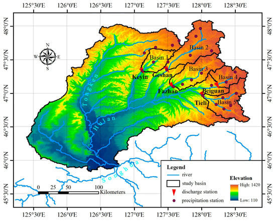
Figure 3.
Hulan River and the analyzed basins in its upper reaches.
Table 4.
List of basins selected for the analysis.
The data required for the tests included a digital elevation model (DEM), land cover, soil property, discharge, and meteorological data. A 3-arc-second DEM was downloaded from the Geospatial Data Cloud [42]. The land cover type data were represented by data downloaded from the website [43], and the database classifies the global land cover into 17 types at a 1-km resolution. The data representing the soil properties were provided by the HWSD [44]. For this study, the utilized daily precipitation and discharge data were provided by the China Hydrologic Yearbook, and the daily meteorological data (except the precipitation data) were downloaded from the National Weather Information Center [45].
3.2. Experiment Design
In our study, 11 majority parameters were calibrated by two schemes: (1) directly calibrated using the ranges listed in Table 1 (denoted as Scheme 1). (2) the parameters were initially estimated as arithmetic averages at 30 arc seconds using the soil moisture characteristics calculated using the S, C, and OC contents from the HWSD (denoted as Scheme 2). These priori parameters of Scheme 2 had to be further adjusted slightly, and the FS was used in all schemes.
In this study, 5-year data was used in the calibration process, and the remaining data (4–5 years) were used for the validation. The Nash-Sutcliffe model efficiency coefficient (NSEC) [46] was used to assess the goodness of fit of the simulated flows:
where Qi,obs is the observed discharge on the ith day, in m3·s−1; Qi,sim is the simulated discharge on the ith day, in m3·s−1; and is the average of all the daily observed discharges, in m3·s−1.
In addition to NSEC, the considered statistical indicators also included the linear correlation coefficient (R) and root mean square error (RMSE) between the observed and simulated daily discharges.
4. Results
4.1. Parameter Applicability
The accuracy statistics of the hydrographs simulated using the calibrated and HWSD data-derived parameters are shown in Table 5. As seen in the table, the directly calibrated parameters (Scheme 1) usually produced higher accuracies (NSEC = 0.66~0.88), although this gain was not extremely significant when compared with the use of the HWSD data-derived parameters (Scheme 2, NSEC = 0.65~0.86). For all basins, the simulation performances under the two schemes were similar. When the NSEC was larger, the other statistical indicators were also better (i.e., R was larger and the RMSE was smaller). However, differences could be seen in the simulation accuracies among different basins. Among the analyzed basins, the discharge simulation results obtained for the Tieli station were the best, the simulation results derived for the Geshan station were the worst, and the results obtained for the other three stations were moderate. In general, the simulation results obtained when using HWSD data-derived parameters were not extremely different from those derived using the calibrated parameters, and this result indicates that it is feasible to use HWSD-listed soil properties to derive the major parameters of the SAC-SMA model. This result shows that in areas lacking soil databases such as STATSGO and SSURGO, HWSD data can be used to derive the major parameters required by the SAC-SMA model.
Table 5.
Accuracy statistics of hydrographs simulated using calibrated and HWSD data-derived parameters for the analyzed basins.
It can be seen from the observed and simulated hydrographs shown in Figure 4 that the performances of the two schemes when simulating the discharge process were generally similar. However, both of the two schemes cannot perform well when simulating peak runoff in some periods (see Figure 4d,e). There are two possible reasons for this phenomenon. First, the data from only 25 precipitation stations were available (see Figure 3), and the daily precipitation and discharge data were not sufficient to accurately simulate the temporal and spatial changes in rainfall and runoff. Second, the daily series of discharge in these five basins changed drastically, and the ratios of the interannual maximum peak flow reached a maximum of 5.6 to 13.0 (see Table 4). Nevertheless, under the available data conditions, the simulation results of the model were still acceptable.
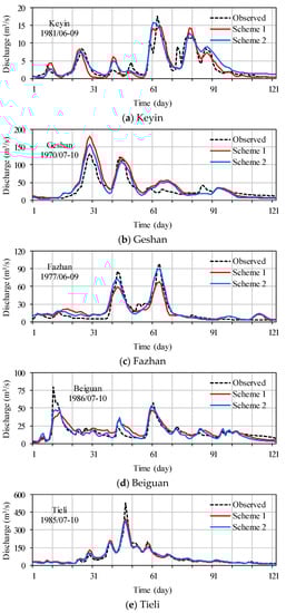
Figure 4.
Observed and simulated hydrographs derived using the calibrated and HWSD data-derived parameters to represent the 5 hydrologic stations.
4.2. Parameter Transferability
In the Radar diagram shown in Figure 5, each basin has transferred its parameters to the other 4 basins; thus, there are 20 parameter transfer results under each scheme. After the parameters were transferred, the simulation accuracies of each basin under all schemes were reduced. Compared with Scheme 1, the NS and R values of Scheme 2 are larger and the RMSE values are smaller, indicating that the parameters of Scheme 2 have better transferability (see Figure 5). Under Scheme 1, the model parameters directly calibrated contain obvious uncertainties (see Figure 6a), although these parameters do make the model achieve slightly better simulation results than Scheme 2 (see Table 5). However, in Scheme 2, the model parameters were derived from the HWSD-listed soil physical properties, and the spatial consistency of these soil physical properties ensures the relative stability of the model parameters (see Figure 6b). Therefore, Scheme 2, in which HWSD data-derived parameters were used, was the best parameter-transfer option in practice.
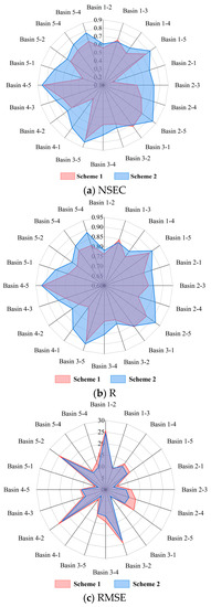
Figure 5.
Radar diagram showing three statistical indicators (NSEC, R, and RMSE) of parameter transitivity (in this figure, the first number after “basin” is the basin code that provided the parameters, and the second number represents the basin code that accepted the parameters.).
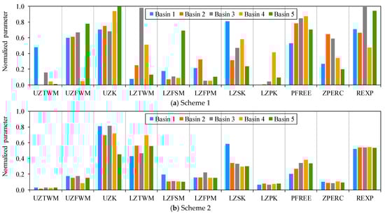
Figure 6.
Variations in the normalized parameters derived under the two schemes.
It was also found that the parameter-transfer quality has no significant relationship with the previous simulation accuracy of the analyzed basins. In the following text, the NSEC is used to discuss the parameter-transfer results of the two schemes, as shown in Figure 7. First, the simulation accuracy of the basin providing the transferred parameters did not determine the simulation qualities of the other basins using those parameters. For example, in Scheme 1 Basin 5 had the largest NSEC (see Table 5); however, the simulation accuracy of Basin 1 obtained under Scheme 1 after using the parameters derived for Basin 5 (NSEC = 0.36, see Figure 7a) was much lower than the simulation accuracy of the same basin after using the parameters obtained for Basin 3 (NSEC = 0.73, see Figure 7a). Basin 2 had the smallest NSEC value among all schemes (see Table 5); however, when its parameters were transferred to the other basins, the simulation results of other basins were not the worst. Second, when other basin parameters were adopted, the basin simulation accuracy was not significantly related to the simulation accuracy obtained before the parameters were transferred. For example, in all schemes, the NSEC value obtained for Basin 1 was greater than that derived for Basin 3 (see Table 5). However, when the parameters of other basins were applied, the simulation accuracies of Basin 1 were lower than or equal to that of Basin 3 in most cases; only in Scheme 2 (NSEC = 0.74, see Figure 7b) was the accuracy higher than that of Basin 3 (NSEC = 0.71, see Figure 7b) when the parameters derived for Basin 4 were applied.
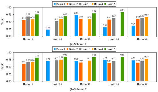
Figure 7.
The NSEC values were used to compare the parameter transferability qualities under the two schemes (in this figure, # indicates the basin that provides parameters to the other basin).
5. Discussion
This article provides a method for estimating soil moisture characteristics using HWSD data. This method can derive the major parameters of the SAC-SMA model at the grid scale and then count these parameters to obtain basin averages. In this method, the S, C, and OC contents listed in the HWSD were used alongside formulas to calculate the soil moisture characteristics. The advantage of this method was that the soil moisture characteristics of any grid could be estimated. The potential application of the second method was beneficial with regard to the development of the conceptual SAC-SMA model into a finer-resolution, high-dimensional grid model.
Compared to the directly calibrated parameters, the HWSD data-derived parameters had better transferability and allowed the SAC-SMA model to achieve similar simulation accuracies in this study. This conclusion is similar to that of Koren et al. [7], although the number of soil layers, the soil profile depth, and the USDA soil texture classification of the HWSD are different from those of STATSGO and SSUGO. Although the HWSD is still very coarse compared to other soil databases, such as STATSGO and SSURGO, the publicly available HWSD may currently be a preferred soil database for deriving the major parameters of the SAC-SMA model in regions outside the United States.
Parameter calibration is an important step in the utilization and development of a hydrologic model for hydrologic simulation. The calibration of hydrologic model parameters usually requires a large amount of hydrometeorological data, and it is extremely difficult to estimate physical parameters, especially in basins that are typically data-poor or ungauged on the ground. The priori parameter sets derived from HWSD soil property data can reduce the manual calibration effort and/or accelerate the automatic calibration process, reduce the calibration uncertainty, and provide valuable spatially consistent parameters for ungauged basins. These spatially consistent and physically reasonable parameter sets are especially suitable for flood simulations and flood forecasting in small watersheds that lack calibration data (such as discharge data).
6. Conclusions
In this study, we developed a parameter-derivation strategy for the SAC-SMA model mainly based on HWSD soil property information and verified the applicability of this strategy in improving the performance of the model when runoff simulating five basins. Based on the results, we obtained the following conclusions.
- (1)
- The directly calibrated SAC-SMA model parameters have obvious uncertainties; specifically, the spatial consistency and transferability of these parameters are not good.
- (2)
- The HWSD soil data can be used to derive the major parameters of the SAC-SMA model and allowed the SAC-SMA model to achieve a similar simulation accuracy as that obtained using directly calibrated parameters.
- (3)
- Compared with the directly calibrated parameters, the parameters derived from the HWSD soil data had better transferability.
Therefore, further research should give more attention to updated HWSD versions and the coupling applications of the HWSD and other datasets to improve the quality-derived SAC-SMA model parameters.
Author Contributions
Conceptualization, B.W., J.H. and X.G.; methodology, B.W. and J.H.; software, B.W.; validation, H.S. and S.G.; formal analysis, J.H. and X.B.; investigation, H.S. and S.G.; writing—original draft preparation, B.W., Z.W. and X.B.; writing—review and editing, B.W. and X.J. All authors have read and agreed to the published version of the manuscript.
Funding
This research was supported by the National Natural Science Foundation of China (51009026), the National Key Research and Development Program of China (2016YFC040010101) and the Natural Science Foundation of Heilongjiang Province, China (LH2021E009).
Data Availability Statement
Not applicable.
Acknowledgments
We would like to extend our gratitude to Robert Horton from Iowa State University for his efforts to improve this manuscript.
Conflicts of Interest
The authors declare no conflict of interest.
Appendix A
Below are the SAC-SMA model major parameter and soil moisture characteristic relationships as they appeared in Koren et al. [7,8] and Anderson et al. [19].
Upper-layer parameters:
Lower-layer parameters:
Percolation parameters:
Upper-layer depth: percolation parameters:
where n is an empirical exponent; Ds is the stream channel density; Δt is the time step, and in the SAC-SMA model, it is equal to 24 h; and θwp,sand is the sand wilting point, in cm−3.
References
- Li, Z.; Li, X.; Wang, J. Causes of spatial mismatch between grain production and water resources: Based on the theory of comparative advantage. J. China Agric. Univ. 2022, 27, 12–29. (In Chinese) [Google Scholar]
- Liu, Z.; Zhao, X.; Zuo, L.; Zhang, Z.; Wang, X.; Xu, J.; Yi, L. Analysis of water resources effect under the pattern optimization of major crops in China. Acta Geogr. Sin. 2023, 78, 746–761. (In Chinese) [Google Scholar]
- Arkesteijn, L.; Pande, S. On hydrological model complexity, its geometrical interpretations and prediction uncertainty. Water Resour. Res. 2013, 49, 7048–7063. [Google Scholar] [CrossRef]
- Elsanabary, M.H.; Gan, T.Y. Evaluation of climate anomalies impacts on the Upper Blue Nile Basin in Ethiopia using a distributed and a lumped hydrologic model. J. Hydrol. 2015, 530, 225–240. [Google Scholar] [CrossRef]
- Katsanou, K.; Lambrakis, N. Modeling the Hellenic karst catchments with the Sacramento Soil Moisture Accounting model. Hydrogeol. J. 2017, 25, 757–769. [Google Scholar] [CrossRef]
- Wijayarathne, D.B.; Coulibaly, P. Identification of hydrological models for operational flood forecasting in St. John’s, Newfoundland, Canada. J. Hydrol.—Reg. Stud. 2020, 27, 100646. [Google Scholar] [CrossRef]
- Koren, V.; Smith, M.; Duan, Q. Use of a priori parameter estimates in the derivation of spatially consistent parameter sets of rainfall-runoff models. Calibration Watershed Model. 2003, 6, 239–254. [Google Scholar]
- Koren, V.; Smith, M.; Wang, D.; Zhang, Z. Use of soil property data in the derivation of conceptual rainfall-runoff model parameters. In Proceedings of the 15th Conference on Hydrology, American Meteorological Society, Long Beach, CA, USA, 9–14 January 2000. [Google Scholar]
- Frances, F.; Velez, J.I.; Velez, J.J. Split-parameter structure for the automatic calibration of distributed hydrological models. J. Hydrol. 2007, 332, 226–240. [Google Scholar] [CrossRef]
- Madsen, H. Parameter estimation in distributed hydrological catchment modelling using automatic calibration with multiple objectives. Adv. Water Resour. 2003, 26, 205–216. [Google Scholar] [CrossRef]
- Beck, H.E.; van Dijk, A.I.J.M.; de Roo, A.; Miralles, D.G.; McVicar, T.R.; Schellekens, J.; Bruijnzeel, L.A. Global-scale regionalization of hydrologic model parameters. Water Resour. Res. 2016, 52, 3599–3622. [Google Scholar] [CrossRef]
- Mizukami, N.; Clark, M.P.; Newman, A.J.; Wood, A.W.; Gutmann, E.D.; Nijssen, B.; Rakovec, O.; Samaniego, L. Towards seamless large-domain parameter estimation for hydrologic models. Water Resour. Res. 2017, 53, 8020–8040. [Google Scholar] [CrossRef]
- Nemri, S.; Kinnard, C. Comparing calibration strategies of a conceptual snow hydrology model and their impact on model performance and parameter identifiability. J. Hydrol. 2020, 582, 124474. [Google Scholar] [CrossRef]
- Xie, K.; Liu, P.; Zhang, J.Y.; Wang, G.Q.; Zhang, X.J.; Zhou, L.T. Identification of spatially distributed parameters of hydrological models using the dimension-adaptive key grid calibration strategy. J. Hydrol. 2021, 598, 125772. [Google Scholar] [CrossRef]
- Bai, P.; Liu, X.M.; Xie, J.X. Simulating runoff under changing climatic conditions: A comparison of the long short-term memory network with two conceptual hydrologic models. J. Hydrol. 2021, 592, 125779. [Google Scholar] [CrossRef]
- Dakhlaoui, H.; Ruelland, D.; Tramblay, Y. A bootstrap-based differential split-sample test to assess the transferability of conceptual rainfall-runoff models under past and future climate variability. J. Hydrol. 2019, 575, 470–486. [Google Scholar] [CrossRef]
- Tegegne, G.; Kim, Y.O. Modelling ungauged catchments using the catchment runoff response similarity. J. Hydrol. 2018, 564, 452–466. [Google Scholar] [CrossRef]
- Koren, V.; Moreda, F.; Smith, M. Use of soil moisture observations to improve parameter consistency in watershed calibration. Phys. Chem. Earth 2008, 33, 1068–1080. [Google Scholar] [CrossRef]
- Anderson, R.M.; Koren, V.I.; Reed, S.M. Using SSURGO data to improve Sacramento Model a priori parameter estimates. J. Hydrol. 2006, 320, 103–116. [Google Scholar] [CrossRef]
- Gan, T.Y.; Burges, S.J. Assessment of soil-based and calibrated parameters of the Sacramento model and parameter transferability. J. Hydrol. 2006, 320, 117–131. [Google Scholar] [CrossRef]
- Guo, B.; Zhang, J.; Xu, T.; Croke, B.; Jakeman, A.; Song, Y.; Yang, Q.; Lei, X.; Liao, W. Applicability Assessment and Uncertainty Analysis of Multi-Precipitation Datasets for the Simulation of Hydrologic Models. Water 2018, 10, 1611. [Google Scholar] [CrossRef]
- Wang, B.; Huang, J.; Gong, X.; Zhu, S.; Wang, G. Application of Sacramento model calibrated by Free Search algorithm in cold and arid region of northeast China. Trans. Chin. Soc. Agric. Mach. 2016, 47, 171–177. (In Chinese) [Google Scholar]
- FAO; IIASA; ISRIC-World Soil Information; Institute of Soil Science; Chinese Academy of Sciences (ISSCAS); Joint Research Centre of the European Commission (JRC). Harmonized World Soil. Database (Version 1.2); FAO: Rome, Italy; IIASA: Laxenburg, Austria, 2012. [Google Scholar]
- Hu, W.M.; Li, G.; Gao, Z.H.; Jia, G.Y.; Wang, Z.C.; Li, Y. Assessment of the impact of the Poplar Ecological Retreat Project on water conservation in the Dongting Lake wetland region using the InVEST model. Sci. Total Environ. 2020, 733, 139423. [Google Scholar] [CrossRef] [PubMed]
- Jodar-Abellan, A.; Valdes-Abellan, J.; Pla, C.; Gomariz-Castillo, F. Impact of land use changes on flash flood prediction using a sub-daily SWAT model in five Mediterranean ungauged watersheds (SE Spain). Sci. Total Environ. 2019, 657, 1578–1591. [Google Scholar] [CrossRef] [PubMed]
- Pei, H.W.; Liu, M.Z.; Shen, Y.J.; Xu, K.; Zhang, H.J.; Li, Y.L.; Luo, J.M. Quantifying impacts of climate dynamics and land-use changes on water yield service in the agro-pastoral ecotone of northern China. Sci. Total Environ. 2022, 809, 151153. [Google Scholar] [CrossRef] [PubMed]
- Watson, A.; Miller, J.; Kunne, A.; Kralisch, S. Using soil-moisture drought indices to evaluate key indicators of agricultural drought in semi-arid Mediterranean Southern Africa. Sci. Total Environ. 2022, 812, 152464. [Google Scholar] [CrossRef]
- Cosby, B.; Hornberger, G.; Clapp, R.; Ginn, T. A statistical exploration of the relationships of soil moisture characteristics to the physical properties of soils. Water Resour. Res. 1984, 20, 682–690. [Google Scholar] [CrossRef]
- Clapp, R.B.; Hornberger, G.M. Empirical equations for some soil hydraulic properties. Water Resour. Res. 1978, 14, 601–604. [Google Scholar] [CrossRef]
- Armstrong, B.L. Derivation of Initial Soil Moisture Accounting Parameters from Soil Properties for the National Weather Service River Forecast System; NOAA: Washington, DC, USA, 1978. [Google Scholar]
- Saxton, K.E.; Rawls, W.J. Soil water characteristic estimates by texture and organic matter for hydrologic solutions. Soil Sci. Soc. Am. J. 2006, 70, 1569–1578. [Google Scholar] [CrossRef]
- Heaton, L.; Fullen, M.A.; Bhattacharyya, R. Critical analysis of the van Bemmelen conversion factor used to convert soil organic matter data to soil organic carbon data: Comparative analyses in a UK loamy sand soil. Espaço Aberto 2016, 6, 35–44. [Google Scholar] [CrossRef]
- Pribyl, D.W. A critical review of the conventional SOC to SOM conversion factor. Geoderma 2010, 156, 75–83. [Google Scholar] [CrossRef]
- Hong, Y.; Adler, R.F. Estimation of global SCS curve numbers using satellite remote sensing and geospatial data. Int. J. Remote. Sens. 2008, 29, 471–477. [Google Scholar] [CrossRef]
- Zeng, Z.Y.; Tang, G.Q.; Hong, Y.; Zeng, C.; Yang, Y. Development of an NRCS curve number global dataset using the latest geospatial remote sensing data for worldwide hydrologic applications. Remote. Sens. Lett. 2017, 8, 528–536. [Google Scholar] [CrossRef]
- Loveland, T.R.; Reed, B.C.; Brown, J.F.; Ohlen, D.O.; Zhu, Z.; Yang, L.; Merchant, J.W. Development of a global land cover characteristics database and IGBP DISCover from 1 km AVHRR data. Int. J. Remote. Sens. 2000, 21, 1303–1330. [Google Scholar] [CrossRef]
- Penev, K.; Littlefair, G. Free search—A comparative analysis. Inf. Sci. 2005, 172, 173–193. [Google Scholar] [CrossRef]
- Wang, B.; Zhu, S.; Huang, J.; Ding, X.; Gong, X.; Wang, G. GSAC model calibration based on evapotranspiration data from Global Land Data Assimilation System. Trans. Chin. Soc. Agric. Mach. 2018, 49, 232–240. (In Chinese) [Google Scholar]
- Han, S.; Zhao, Y. Analysis of variation trend and mutation characteristics of natural runoff in the upstream of the Hulanhe River basin. Water Resour. Power 2020, 38, 46–50. (In Chinese) [Google Scholar]
- Zhou, G. Study on the intra-annual runoff distribution characteristics in Hulan River basin. Water Resour. Power 2018, 36, 39–43. (In Chinese) [Google Scholar]
- Duan, M.; Feng, J. The change trend of runoff at Lanxi station of Hulan River since 1956. Heilongjiang Water Resour. 2017, 3, 59–61. (In Chinese) [Google Scholar]
- Geospatial Data Cloud (GDC). Available online: http://www.gscloud.cn (accessed on 10 December 2021).
- IGBP DISCover Database. Available online: http://edcwww.cr.usgs.gov/landdaac/glcc/glcc.html (accessed on 20 April 2002).
- Harmonized World Soil Database (HWSD). Available online: https://www.fao.org/soils-portal/data-hub/soil-maps-and-databases/harmonized-world-soil-database-v12/en/ (accessed on 10 December 2021).
- National Weather Information Center (NWIC). Available online: http://data.cma.cn (accessed on 10 December 2021).
- Nash, J.E.; Sutcliffe, J.V. River flow forecasting through conceptual models part I—A discussion of principles. J. Hydrol. 1970, 10, 282–290. [Google Scholar] [CrossRef]
Disclaimer/Publisher’s Note: The statements, opinions and data contained in all publications are solely those of the individual author(s) and contributor(s) and not of MDPI and/or the editor(s). MDPI and/or the editor(s) disclaim responsibility for any injury to people or property resulting from any ideas, methods, instructions or products referred to in the content. |
© 2023 by the authors. Licensee MDPI, Basel, Switzerland. This article is an open access article distributed under the terms and conditions of the Creative Commons Attribution (CC BY) license (https://creativecommons.org/licenses/by/4.0/).