Estimation of Reference Crop Evapotranspiration with Three Different Machine Learning Models and Limited Meteorological Variables

Abstract

Precise reference crop evapotranspiration (ET₀) estimation plays a key role in agricultural fields as it aids in the proper operation and management of irrigation scheduling. However, reliable ET₀ estimation poses a challenge when there is insufficient or incomplete long-term meteorological data at the East Coast Economic Region (ECER), Malaysia, where the economy is highly dependent on agricultural crop production. This study evaluated the performances of different standalone machine learning (ML) models, namely, the light gradient boosting machine (LGBM), decision forest regression (DFR), and artificial neural network (ANN) models using four different combinations of meteorological variables. The incorporation of solar radiation enhanced the accuracy of the standalone ML models, demonstrating the role of energetic factors in the evapotranspiration mechanism. Additionally, both the ANN and LGBM models showed overall satisfactory performances, and were thus recommended them as alternate models for ET₀ estimation. This was owing to their good capability in capturing the non-linearity and interaction process among the meteorological variables. The outcomes of this study will be advantageous to farmers and policymakers in determining the actual crop water demands to maximize crop productivity in data-scarce tropical regions.

1. Introduction

The simultaneous occurrence of evaporation and transpiration gives rise to the concept of evapotranspiration (ET). Both ET and transpiration are governed by factors such as meteorological variables, crop attributes, and ecological variables. ET is comprised of the water loss from the combination of both evaporation and transpiration processes to the atmosphere. ET is a crucial parameter for hydrological and agrometeorological studies, especially in optimizing water usage in the agricultural industry [1,2]. There are various methods for estimating ET, each with its pros and cons depending on itsspecific application and data prerequisites. ET can be measured directly using instruments such as weighting lysimeters and eddy covariance to provide accurate and credible ET data. Despite their high capability in measuring ET, the use of these instruments is challenging to use them for large area field measurements as they are high in maintenance costs and time-consuming [1,3].

Reference crop evapotranspiration (ET₀) is the volume of water that a hypothetical grass reference crop will lose through evaporation and transpiration. This reference crop is assumed to have a uniform height of 0.12 m, a surface resistance of 70 s m⁻¹, and an albedo of 0.23 [4]. The Food and Agriculture Organization (FAO) of the United Nations developed the FAO-56 Penman–Monteith (FAO-56 PM) model and recommended it as the universal approach to estimate ET₀ [5,6]. This model has been extensively compared with various empirical models over different climatic conditions and temporal scales and has consistently been found to be superior. However, its application is limited in many locations around the world due to the requirement of abundant and diverse meteorological variables. These meteorological data are frequently deficient, inaccessible, or of questionable quality, particularly in developing countries [7,8].

The estimation of ET₀ using empirical models with less meteorological variables as inputs has been proposed and validated worldwide [9,10,11]. Yang et al. [12] evaluated eight different empirical ET₀ models across agricultural zones in China. The radiation-based models demonstrated superior performance in comparison to the temperature-based models. According to Mehdizadeh et al. [13], the radiation-based models outperformed mass transfer-based and temperature-based models in Iran. Hamed et al. [14], conversely, came to the conclusion that temperature-based models exhibited superior performance compared to other empirical models in Pakistan. Celestin et al. [15] conducted daily and monthly ET₀ estimations using 32 empirical models and reported that both the World Meteorological Organization and Mahringer models (mass transfer-based models) showed the best performance in northwest China. Another comparison of six empirical models in North Algeria reported that the combination-based models provided more accurate estimations than the radiation- and temperature-based models [7]. It can be inferred from the aforementioned studies that the limitation of the empirical models lies in their consistency, as the performance and accuracy of the models are affected by different climatic conditions. This shortcoming will potentially result in uncertainties in model estimation, making it difficult to apply in data-scarce regions, especially Malaysia.

To address the drawback of the FAO-56 PM model’s high demand for diverse meteorological data and the inconsistency in the simple empirical models, various machine learning (ML) models have been applied as they are more economical and easily applicable. Therefore, the ML models have become favourable substitution options over direct or indirect methods. A prominent trend has emerged in the application of ML models for ET₀ estimation, especially in the regions where meteorological data are insufficient or inaccessible. For example, Zhang et al. [16] modelled ET₀ using k-nearest neighbours (kNN), RF, ANN, light gradient boosting machine (LGBM), and temporary convolutional neural network (TCN) models with limited meteorological data in northern China. These standalone ML models yielded more accurate ET₀ estimations compared to the empirical models. Furthermore, Rai et al. [17] investigated the estimation of monthly ET₀ using the SVM, M5P model tree, and RF models in India. The SVM model surpassed the other ML and empirical models in terms of statistical performance. Liu et al. [18] conducted a comparison between the SVM, RF, and extreme learning models (ELM) to estimate daily ET₀ in the Yellow River Basin, China. The findings indicated that the RF model demonstrated superior performance compared to all of the examined models, followed by the ELM. In comparison, the empirical models were found to overestimate and underestimate ET₀. It can be highlighted that the standalone ML models demonstrated better performance and accuracy compared to the empirical models.

ANNs, which are known as one of the earliest and widely used approaches for retrieving information from non-linear data, have been extensively applied due to their exceptional capability to outline input–output relationships with good accuracy and without any understanding of the underlying physical processes [19]. Antonopoulos and Antonopoulos [20] put forward an ANN model that incorporated a backpropagation algorithm, and subsequently implemented the model to estimate ET₀. The findings confirmed that the ANN model provided reliable and precise ET₀ estimation. Ferreira et al. [21] employed ANN and SVM models to predict ET₀ in Brazil. The findings demonstrated that the ANN outperformed the SVM and other empirical models that were examined. Dimitriadou et al. [22] evaluated the potential for daily ET₀ estimation during the summer and wintertime in Greece. The findings suggested that the multi-layer perceptron outperformed the radial basis function, and the ANNs with fewer meteorological inputs could be good predictive ET₀ models. Moreover, Maqsood et al. also highlighted the high accuracy of ET₀ estimation using ANNs (MLP, LSTM and CNN) in the western and eastern part of Prince Edward Island [8]. However, ANNs are prone to overfitting as they require a large quantity of data [23]. An excessive number of neurons will prolong the duration of the network’s training, and subsequently lead to overfitting [19].

The LGBM model was developed by Microsoft [24], and it has been applied in many fields due to its high accuracy, fast and efficient computational speed, as well as regularization techniques to reduce overfitting. Fan et al. [25] were the pioneer batch of researchers who adopted the LGBM model to estimate ET₀. The LGBM model was deemed superior to the other ML models. A comparative analysis by Zhou et al. [26], studying the performances of daily ET₀ estimation in China, concluded with reliable model stability and prediction potential of both the CatBoost and LGBM models.

The deficiency in comprehensive and qualitative meteorological data at both the spatial and temporal scales has been a predicament in the East Coast Economic Region (ECER) of Malaysia. The lack of quality meteorological data has affected the farmers’ ability to provide detailed information about the actual crop water demand, resulting in reduced yields and crop failure. Consequently, it is challenging for farmers to optimize irrigation scheduling and agricultural water management for the ECER, where agricultural activities are the main economic source to achieve its huge potential to improve crop production [27]. In this context, the current study involves an investigation of ET₀ estimation using different standalone ML models, including ANN, decision forest regression (DFR), and LGBM models. The standalone ML models were examined using four scenarios with different meteorological variables as the inputs (scenario 1: maximum air temperature (Tmax), minimum air temperature (Tmin), and mean air temperature (Tmean); scenario 2: Tmax, Tmin, Tmean, and solar radiation (Rs); scenario 3: Tmax, Tmin, Tmean, Rs, and wind speed (WS); scenario 4: Tmax, Tmin, Tmean, Rs, WS, and RHmean). Additionally, the best ET₀ model was identified for each specific meteorological data input scenario by comparing the standalone ML models against the FAO-56 PM model through statistical performance tests. The findings of this study presented the performances of the ML models for accurate ET₀ estimations with limited meteorological data, subsequently easing the decision-making process for policymakers by disclosing comprehensive information about the crop water requirements and will enhance the productivity of crop production in the ECER.

2. Materials and Methods

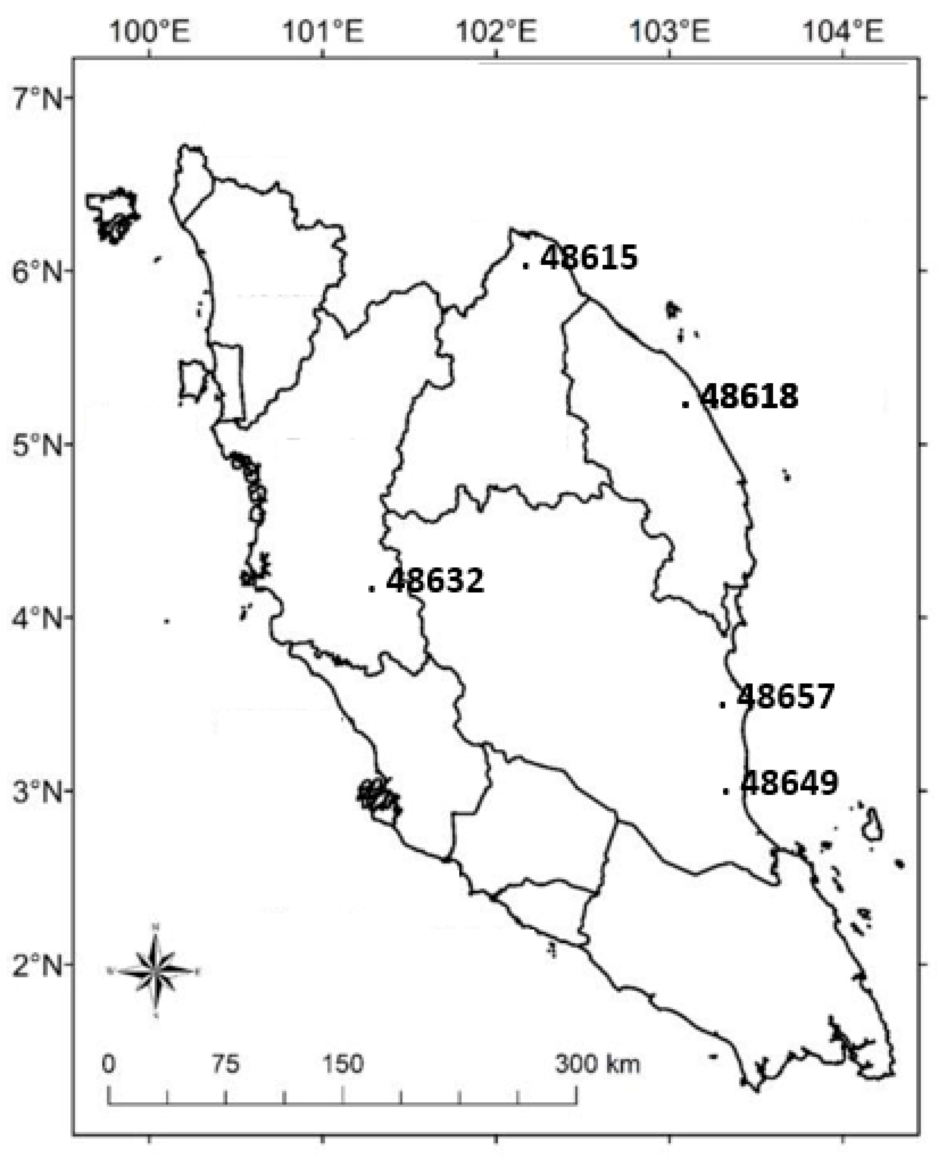
2.1. Study Area

The ECER comprises three states, namely, Pahang, Terengganu, and Kelantan. With an area of 66,000 km², the ECER accounts for 34% of the total agricultural area in Peninsular Malaysia. Crop production, such as oil palm, rubber, and paddy field, covers a total area of 2.2 million ha [28]. Accurate ET₀ estimation is crucial to improve the crop productivity and reduce poverty intensity in this region, which has high coverage of agricultural crop productions. Additionally, the tropical climate in the ECER is predominantly affected by the monsoon seasons and climate change. The climate undergoes periodical changes in wind direction due to the northeast and southwest monsoons [29]. The northeast monsoon takes place annually from November to March and is characterized by prevailing easterly to north-easterly wind. During the southwest monsoon (May to September), the prevailing winds blow from the southwest [30].

The daily meteorological data, consisting of Tmax, Tmin, Tmean, Rs, WS, and RHmean were collected from the Malaysian Meteorological Department. Figure 1 and

Table 1. The details of each meteorological station.

Station Code	Station Name	Record Period	Duration	Latitude	Longitude
48618	Kuala Terengganu	2000–2019	20	05°23′ N	103°06′ E
48632	Cameron Highland	2000–2019	20	04°28′ N	101°22′ E
48615	Kota Bahru	2000–2019	20	06°10′ N	102°18′ E
48657	Kuantan	2000–2019	20	03°46′ N	103°13′ E
48649	Muadzam Shah	2000–2019	20	03°03′ N	103°05′ E

depict the geographical locations and information for each meteorological station in the ECER, respectively.

2.2. FAO-56 Penman–Monteith Model

The FAO-56 PM model is the most universally accepted model for ET₀ estimation in different climatic conditions and regions [18,21]. It was used as the benchmark for comparison with the standalone ML models. The equation is presented below [4]:

$$E{T}_0=\frac{0.480\mathsf{\Delta }\left(R_n-G\right)+\gamma \frac{900}{ T_{mean}+273}{u}_{2 }\left(e_{s }-e_a\right)}{\mathsf{\Delta }+\gamma \left(1+0.34 u_{2 }\right)}$$

(1)

where $R_n$ is the net radiation of the crop surface (${\mathrm{MJ}\mathrm{m}}^{-2}{\mathrm{day}}^{-1}$); ∆ is the slope vapor curve ($\mathrm{kPa}°{\mathrm{C}}^{-1}$); $T_{mean}$ is the daily mean air temperature at 2 m height $\left(°\mathrm{C}\right)$; $u_{2 }$ is the wind speed at 2 m height $({\mathrm{m}\mathrm{s}}^{-1}$); G is the soil heat flux density (${\mathrm{MJ}\mathrm{m}}^{-2}{\mathrm{day}}^{-1}$);$e_a$ is the actual vapor pressure (kPa); $e_s$ is the saturation vapor (kPa), and γ is the psychrometric constant ($\mathrm{kPa}°{\mathrm{C}}^{-1}$).

2.3. Standalone Machine Learning Models

In this study, three standalone ML models (DFR, ANN, and LGBM) were applied for the ET₀ estimation. The FAO-56 PM model was employed to compare their ET₀ performances. These models are briefly described below:

2.3.1. Decision Forest Regression (DFR)

The DFR model operates as a non-parametric model that evaluates each instance by navigating through a binary tree data structure until it arrives at a leaf node (decision). DFR uses the RF algorithm developed by Leo Breiman [31]. This model aggregates the decision of multiple trees that are trained on various subsets of data. Each individual decision tree (weak learner) produces its own prediction [19]. DFR is adept in terms of both computational speed and memory usage for both training and prediction purposes. It has the ability to express non-linear decision boundaries and reduce the impact of noisy features. More information on the DFR model can be acquired from Raza et al. [32].

2.3.2. Light Gradient Boosting Model (LGBM)

The LGBM model is an extensively employed technique for solving regression problems introduced by Friedman [33]. It uses decision stumps or regression trees as weak classifiers. The LGBM model is able to detect non-linear transformations, handle categorical variables, exhibit computational stability, and demonstrate exceptional scalability [34,35]. The efficiency and scalability of the LGBM model are enhanced by the gradient-based one-side sampling (GOS) and the exclusive feature bundling techniques. The GOS technique addresses class imbalance in the data to achieve more model accuracy. Moreover, the exclusive feature bundling utilizes a histogram-based algorithm to categorize related feature values into exclusive sets to improve computational efficiency. Additional information about the LGBM model can be acquired in [35].

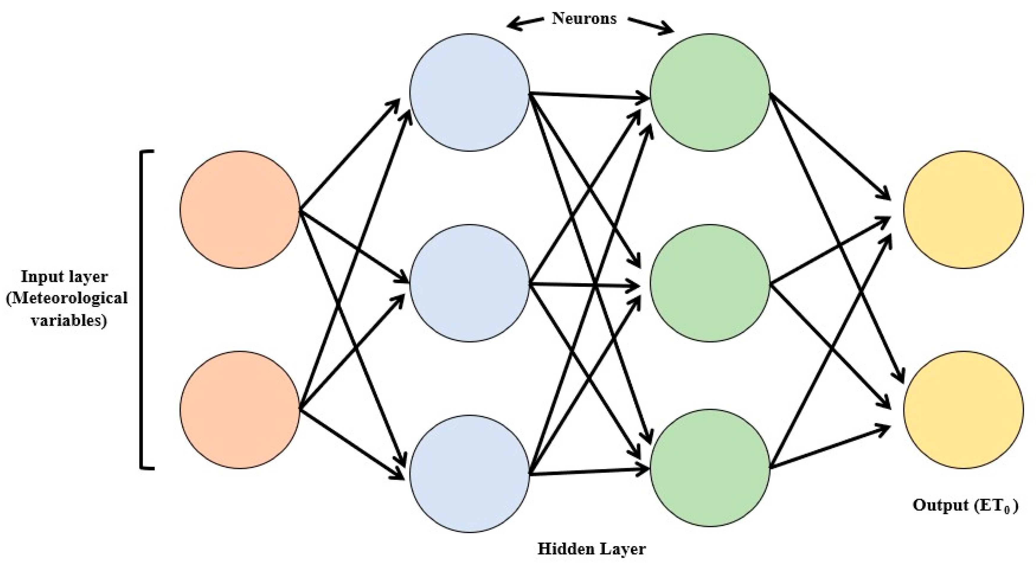
2.3.3. Artificial Neural Network (ANN)

The ANN model comprises multiple interconnected neurons that are organized into layers and connected by weights. It has three distinct layers, namely, the input, hidden, and output layers. The input layer receives the meteorological data while the output layer exhibits ET₀. The hidden layer, which is located between the input and output layers, processes the data, and plays a crucial role in handling non-linear data. Each neuron is linked to either the preceding or succeeding layer. The ANN model undergoes multiple rounds of training while adjusting the number of neurons in each layer to prevent overfitting [21,36]. Figure 2 shows the typical three layers in the ANN structure.

2.4. Model Development and Performance Evaluation

The daily ET₀ in the ECER region was predicted using the standalone ML models (DFR, LGBM, and ANN), each using meteorological variables (Tmax, Tmin, Tmean, Rs, WS, and RHmean) as input variables.

Table 2. Correlation matrix between ET₀ and meteorological variables.

	Tmax	Tmin	Tmean	RH	WS	Rs	ET0
Tmax	1.00
Tmin	0.93	1.00
Tmean	0.97	0.98	1.00
RH	−0.75	−0.64	−0.72	1.00
WS	−0.02	0.06	0.03	−0.25	1.00
Rs	0.43	0.24	0.33	−0.54	0.15	1.00
ET0	0.73	0.59	0.67	−0.76	−0.14	0.91	1.00

displays a matrix of correlation coefficients between the meteorological variables and ET₀. It was used to determine the degree of the relationship between meteorological variables and ET₀. According to the results from Table 2, the correlation coefficient between ET₀ and Rs was higher (0.91) compared to the other meteorological variables. This suggests that Rs has a stronger influence on ET₀ than the other meteorological variables. The second highest correlation of 0.73 was obtained between ET₀ and Tmax. Rs and air temperature (T) are the main drivers of the ET₀ process. With values of −0.76 and −0.14, the RHmean and WS were the only meteorological variables negatively corelated with ET₀.

This study created four different input combinations of meteorological variables and analysed them using standalone ML models. These combinations of meteorological variables were grouped based on the correlation coefficients. For instance, scenario 1 (Tmax, Tmin, and Tmean); scenario 2 (Tmax, Tmin, Tmean, and Rs); scenario 3 (Tmax, Tmin, Tmean, Rs, and WS); scenario 4 (Tmax, Tmin, Tmean, Rs, WS, and RHmean). These combinations constitute the energetic (Rs and T) and aerodynamic (WS and RH) parts of the ET process. The objective of these scenarios was to evaluate how well these ML models perform using varying combinations of meteorological variables. In addition, twenty years of daily meteorological variables were separated into two sets: 70% was utilized for training, while the remaining 30% was used for testing.

The performances of different standalone ML models were assessed using the mean absolute error (MAE), root mean square error (RMSE), relative absolute error (RAE), relative squared error (RSE), and coefficient of determination (R²). The equations are given as follow:

$$MAE=\frac{{{\displaystyle \sum }}_{i=1}^n\left(S_i-O_i\right)}{n}$$

(2)

$$RMSE=\sqrt{\frac{{{\displaystyle \sum }}_{i=1}^n{\left(S_i-O_i\right)}^2}{n}}$$

(3)

$$RAE=\frac{{{\displaystyle \sum }}_{i=1}^n\left(S_i-O_i\right)}{O_i}$$

(4)

$$RSE=\frac{{{\displaystyle \sum }}_{i=1}^n{(S_i-O_i)}^2}{\sum {(\overline{O_i}-O_i)}^2}$$

(5)

$$R^2={\left[\frac{{{\displaystyle \sum }}_{i=1}^n\left(S_i-\overline{S_i}\right)\left(O_i-\overline{O_i}\right)}{\sqrt{\sum {(S_i-\overline{S_i})}^2}\sqrt{\sum {(O_i-\overline{O_i})}^2}}\right]}^2$$

(6)

where $S_i$ represents predicted ET₀ values; $\overline{S_i}$ is the mean predicted ET₀ values; $O_i$ represents observed ET₀ values; and $\overline{O_i}$ is the mean ET₀ observed values.

3. Results

3.1. Standalone Machine Learning Models

Three standalone ML models were tested using four different scenarios of meteorological variables.

Table 3. Statistical evaluation of DFR model with different meteorological variables for testing subsets.

Station	Model	MAE	RMSE	RAE	RSE	R2
Cameron Highlands	DFR 1	0.496	0.654	0.641	0.442	0.558
	DFR 2	0.050	0.081	0.066	0.007	0.993
	DFR 3	0.040	0.062	0.051	0.004	0.996
	DFR 4	0.028	0.045	0.036	0.002	0.998
Kota Bahru	DFR 1	0.475	0.558	0.580	0.420	0.580
	DFR 2	0.304	0.388	0.540	0.349	0.651
	DFR 3	0.210	0.110	0.453	0.280	0.720
	DFR 4	0.190	0.110	0.453	0.224	0.776
Kuala Terengganu	DFR 1	0.659	0.807	0.890	0.236	0.764
	DFR 2	0.120	0.183	0.162	0.039	0.961
	DFR 3	0.086	0.128	0.115	0.019	0.981
	DFR 4	0.038	0.056	0.051	0.004	0.996
Kuantan	DFR 1	0.875	0.945	0.980	0.409	0.591
	DFR 2	0.704	0.927	0.925	0.358	0.642
	DFR 3	0.710	0.855	0.939	0.320	0.680
	DFR 4	0.690	0.812	0.857	0.303	0.700
Muadzam Shah	DFR 1	0.775	0.768	0.580	0.310	0.690
	DFR 2	0.604	0.388	0.540	0.287	0.713
	DFR 3	0.610	0.10	0.453	0.250	0.750
	DFR 4	0.593	0.210	0.453	0.214	0.786

,

Table 4. Statistical evaluation of LGBM model with different meteorological variables.

Station	Model	MAE	RMSE	RAE	RSE	R2
Cameron Highlands	LGBM 1	0.465	0.609	0.600	0.384	0.616
	LGBM 2	0.049	0.078	0.063	0.006	0.994
	LGBM 3	0.036	0.055	0.047	0.003	0.997
	LGBM 4	0.021	0.032	0.027	0.001	0.999
Kota Bahru	LGBM 1	0.275	0.463	0.581	0.393	0.607
	LGBM 2	0.223	0.350	0.311	0.289	0.711
	LGBM 3	0.211	0.328	0.301	0.250	0.750
	LGBM 4	0.209	0.315	0.253	0.206	0.794
Kuala Terengganu	LGBM 1	0.625	0.766	0.884	0.700	0.320
	LGBM 2	0.114	0.174	0.153	0.037	0.964
	LGBM 3	0.080	0.121	0.107	0.017	0.983
	LGBM 4	0.029	0.041	0.040	0.002	0.998
Kuantan	LGBM 1	0.444	0.691	0.585	0.369	0.631
	LGBM 2	0.565	0.609	0.601	0.332	0.668
	LGBM 3	0.348	0.346	0.364	0.290	0.710
	LGBM 4	0.323	0.302	0.339	0.256	0.744
Muadzam Shah	LGBM 1	0.685	0.298	0.304	0.221	0.779
	LGBM 2	0.342	0.284	0.299	0.182	0.818
	LGBM 3	0.284	0.239	0.166	0.152	0.847
	LGBM 4	0.101	0.132	0.107	0.095	0.905

and

Table 5. Statistical evaluation of ANN model with different meteorological variables for testing subsets.

Station	Model	MAE	RMSE	RAE	RSE	R2
Cameron Highlands	ANN 1	0.469	0.615	0.606	0.392	0.608
	ANN 2	0.083	0.123	0.107	0.156	0.984
	ANN 3	0.818	0.120	0.106	0.015	0.985
	ANN 4	0.037	0.059	0.477	0.004	0.996
Kota Bahru	ANN 1	3.832	4.650	0.807	0.643	0.356
	ANN 2	1.408	2.102	0.297	0.132	0.868
	ANN 3	0.999	1.807	0.210	0.097	0.903
	ANN 4	0.493	1.634	0.104	0.079	0.921
Kuala Terengganu	ANN 1	0.652	0.778	0.879	0.711	0.289
	ANN 2	0.170	0.217	0.229	0.055	0.944
	ANN 3	0.107	0.147	0.144	0.025	0.975
	ANN 4	0.075	0.091	0.102	0.010	0.990
Kuantan	ANN 1	0.700	0.911	0.807	0.202	0.798
	ANN 2	0.501	0.689	0.194	0.068	0.932
	ANN 3	0.361	0.542	0.269	0.119	0.881
	ANN 4	0.359	0.685	0.207	0.103	0.897
Muadzam Shah	ANN 1	0.765	0.976	0.791	0.311	0.689
	ANN 2	0.452	0.583	0.152	0.065	0.935
	ANN 3	0.303	0.444	0.134	0.033	0.967
	ANN 4	0.166	0.238	0.106	0.016	0.984

display the result of the models’ performances, and Figure 3, Figure 4 and Figure 5 illustrate the scatter plots of the observed and simulated ET₀ for each model. A good fit was indicated when the scatter points (data) aligned with the diagonal trend line, while a poor fit was indicated when they deviated from the trend line. Overall, the models’ performances were found to be the poorest when only the Tmax, Tmin, and Tmean were used as input variables in the first scenario, where the data points showed more scattering. This was because these models could not effectively describe the connections between the meteorological variables and the ET₀ when only one meteorological variable (Tmean) was included. The fourth combination, which used the Tmax, Tmin, Tmean, Rs, WS, and RH, produced the best fit as all data points were aligned with the trend line. These findings supported the correlation between ET₀ and the meteorological variables as previously reported in Table 2.

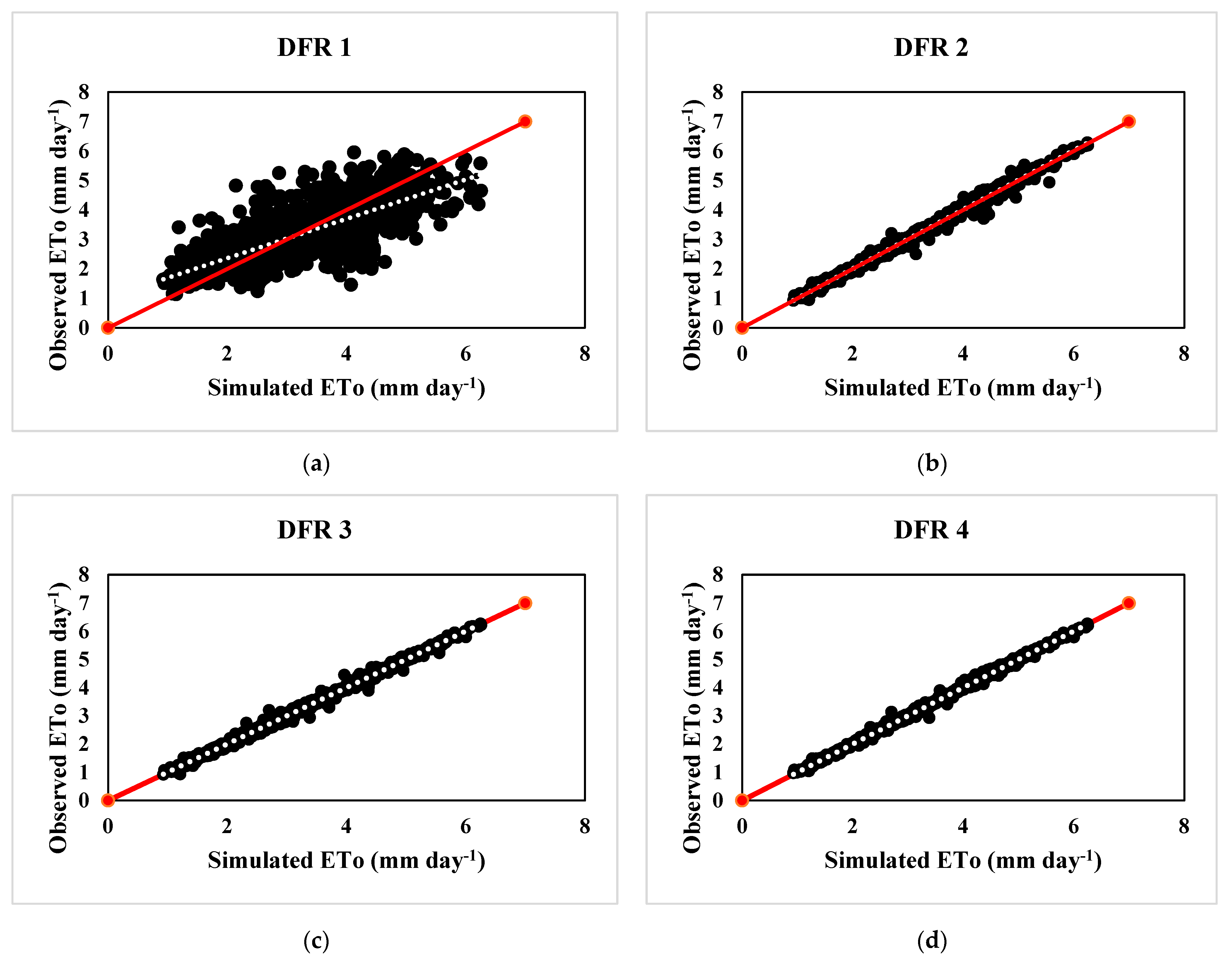
3.2. Performance of Decision Forest Regression Model

Table 3 displays the overall results of the DFR model’s performance. The statistical results of the ET₀ estimation using the DFR model with four combinations of meteorological variables indicated that DFR 4 (scenario 4) obtained the best performance, while DFR 1 (scenario 1) exhibited the lowest performance with only the Tmax, Tmin, and Tmean. A significant improvement in ET₀ estimation was observed for scenario 2. In scenario 2 (DFR 2), more than a 50% improvement in ET₀ estimation was observed at the Cameron Highlands and Kuala Terengganu stations when the solar radiation data were included as input. With respect to scenario 1 (DFR 1), the MAE improved from 0.496 to 0.05 mm day⁻¹, RMSE from 0.645 to 0.081 mm day⁻¹, RAE from 0.641 to 0.066 mm day⁻¹, RSE from 0.442 to 0.007, and R² from 0.558 to 0.993 at the Cameron Highlands station. For the Kuala Terengganu station, the MAE improved from 0.659 to 0.12 mm day⁻¹, RMSE from 0.807 to 0.183 mm day⁻¹, RAE from 0.890 to 0.182 mm day⁻¹, RSE from 0.236 to 0.039, and R² from 0.764 to 0.961. DFR 3 (scenario 3) and DFR 4 (scenario 4) exhibited further improvements at all stations.

In addition, the comparison between the observed and simulated ET₀ values for the DFR model (Cameron Highlands station) is presented in Figure 3. The best result was observed for DFR 4 (scenario 4), where all of the data points occurred along the trend line. In comparison, the data points showed more scattering for DFR 1 (scenario 1), indicating the worst performance. Overall, the DFR model demonstrated a slight tendency for ET₀ overestimation. For the Cameron Highlands, the DFR model overestimated the ET₀ values ranging from 0.13% to 0.91% for all scenarios.

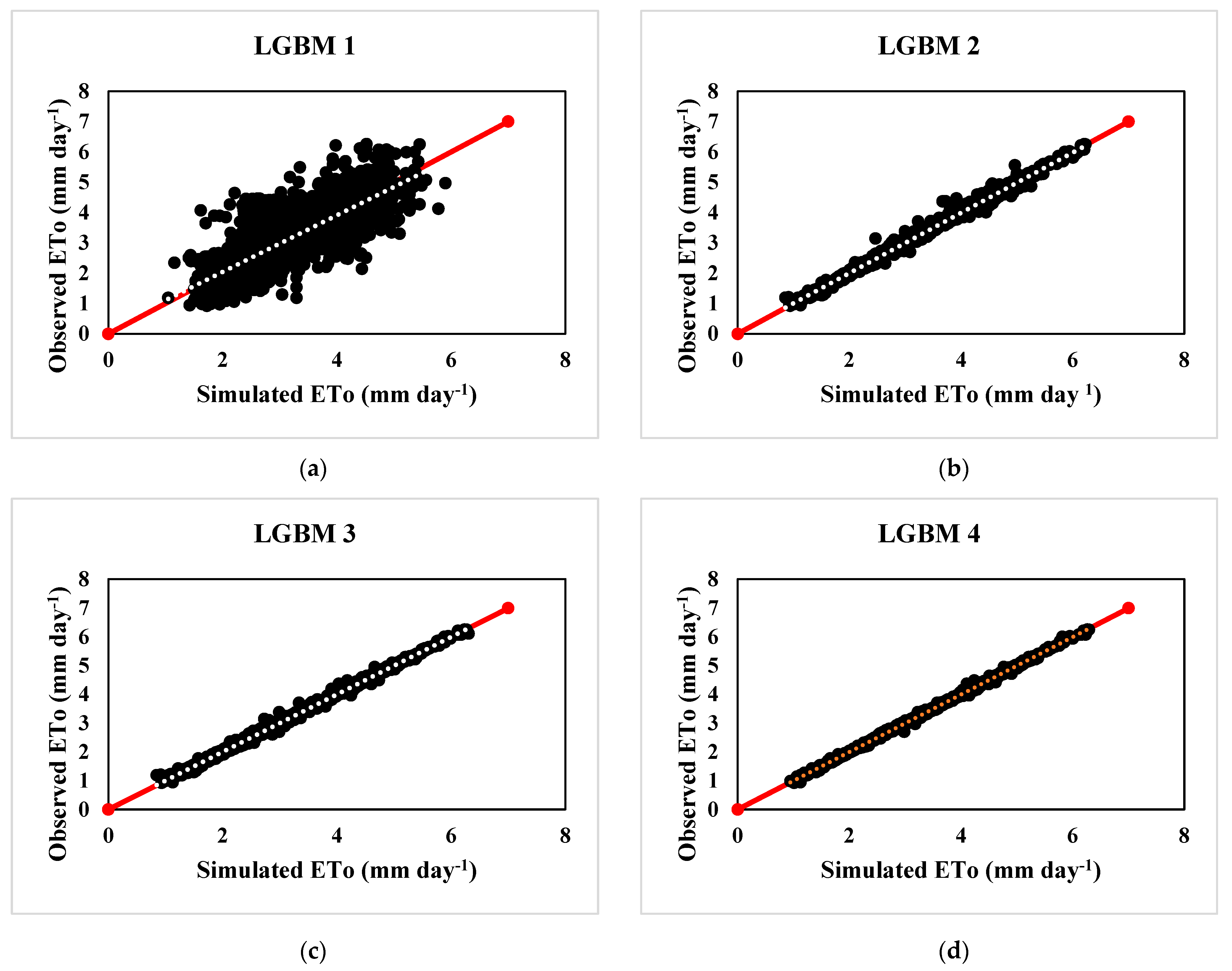
3.3. Performance of Light Gradient Boosting Model

Using the gradient boosting technique, the best results were obtained by setting the learning rate to 1 and the number of estimators to 50. From Table 4, the LGBM model gave the best performance for LGBM 4 (scenario 4). In contrast, the lowest performance occurred in LGBM 1 (scenario 1) for the majority of the stations. Among all stations, the Cameron Highlands, Kota Bahru, and Kuantan stations had the lowest performance, as evidenced by the highest MAE, RMSE, RAE, RSE values, and the lowest R² values. The performance was improved significantly in terms of the MAE, RMSE, RAE, RSE, and R² for LGBM 2 (scenario 2). For instance, with respect to LGBM 1 (scenario 1), the MAE improved from 0.659 to 0.120 mm day⁻¹, RMSE from 0.807 to 0.183 mm day⁻¹, RAE from 0.890 to 0.162 mm day⁻¹, RSE from 0.236 to 0.039, and R² from 0.764 to 0.961 at the Kuala Terengganu station. A further improvement in the LGBM model performance was demonstrated for LGBM 3 and 4 (scenarios 3 and 4) when more meteorological variables were included as input data. The LGBM depicted the best performance for ET₀ estimation in scenario 4 with the lowest RMSE, RAE, and RSE values, as well as the highest R² values across all stations.

The best result was observed for LGBM 4 (scenario 4), where all of the data points occurred along the trend line in Figure 4d. In contrast, scenario 1 (LGBM 1) exhibited the worst performance as the data points showed more scattering in Figure 4a. Overall, the LGBM models demonstrated a slight tendency for ET₀ overestimation. For the Cameron Highlands, the LGBM model overestimated the observed ET₀ values between the range of 0.01% and 0.82% for all scenarios.

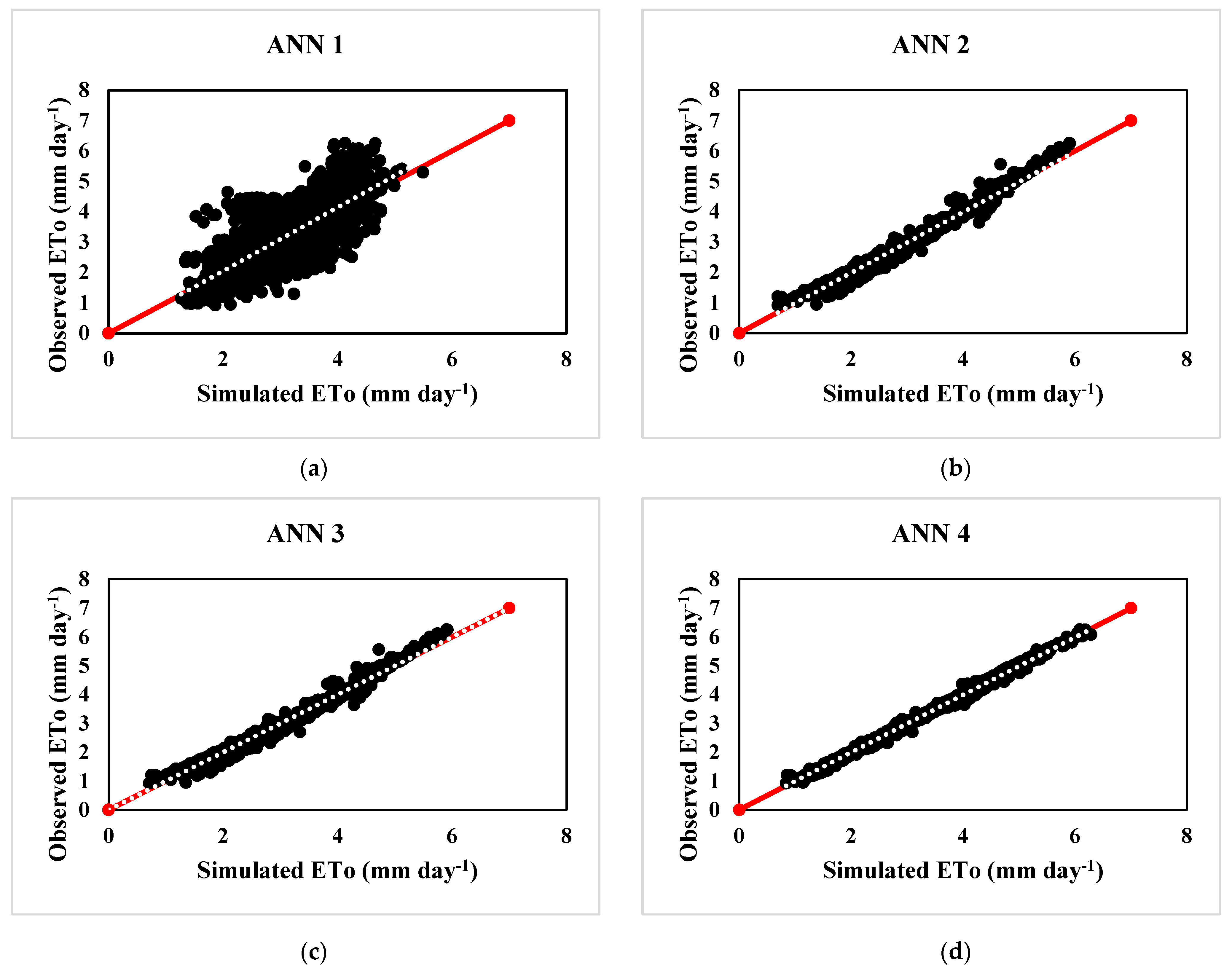
3.4. Performance of Artificial Neural Network Model

According to Table 5, the performance of the ANN model was assessed using four different scenarios based on the availability of the meteorological variables. Among all of the stations, ANN 4 (scenario 4) exhibited the best performance, while ANN 1 (scenario 1), which used only the Tmax, Tmin, and Tmean data as input, showed the poorest performance. The Cameron Highlands, Kuantan, and Muadzam Shah stations had the highest MAE, RMSE, RAE, RSE values and the lowest values of the R², which indicated poor statistical performance of the model. An improvement in ET₀ estimation was observed for ANN 2 (scenario 2), which resulted in a reduction in the MAE, RMSE, RAE, RSE, and an increase in the R² for all stations. For example, at the Kota Bahru station, the MAE improved from 3.832 to 1.408 mm day⁻¹, RMSE from 4.650 to 2.102 mm day⁻¹, RAE from 0.807 to 0.297 mm day⁻¹, RSE from 0.643 to 0.132, and R² from 0.356 to 0.868. A slight improvement could be noticed in ANN 3 and ANN 4. For example, the Cameron Highlands station showed the highest R² value of 0.998 and lowest values in the MAE, RMSE, RAE, and RSE (0.028 mm day⁻¹, 0.045 mm day⁻¹, 0.036, and 0.002, respectively).

It could be observed that ANN 4 (scenario 4) achieved the best result in Figure 5d, as all of the data points occurred along the trend line. In contrast, ANN 1 (scenario 1) showed the worst performance, as the data points were more scattered in Figure 5a. Overall, the ANN model demonstrated a slight tendency for ET₀ overestimation. For the Cameron Highlands station, the ANN model showed a slight underestimation in scenario 1 (3.05%) and a slight overestimation in scenarios 2, 3, and 4 (0.26−0.45%).

4. Discussion

In general, the model estimation accuracy ranked in descending order as ANN > LGBM > DFR. The ANN showed slightly better performance than the LGBM when there were fewer meteorological variables, specifically in scenarios 1, 2, and 3. Its superior performance was due to the backpropagation algorithm, which allowed the ANN to achieve better performance in the non-linear approximation. The ANN can use hidden layers to learn a high-level representation of the data and extract features that are relevant for ET₀ estimation. This can lead to accurate predictions, even when the meteorological variables are limited. Dimitriadou et al. [22] suggested that the ANN model could be a good predictive ET₀ model even with limited meteorological variables as input.

Furthermore, the LGBM model outperformed the other standalone models in scenario 4. This means that the LGBM had an acceptable model stability for estimating the ET₀ in the ECER. When there are full meteorological variables available, it can handle large datasets and high-dimensional data with relative ease. The LGBM can learn from a large number of meteorological variables and identify the most important features for ET₀ estimation. This can lead to more accurate predictions when the input variables are complex and numerous. This finding supports the ideas of Fan et al. [25], who suggested that when using complete meteorological data, the LGBM model performed better than other standalone ML models. Similarly, Wu et al. [35] reported that the LGBM model achieved very close accuracy in ET₀ estimation than the other boosting-based models. Based on these results, the ANN and LGBM models are recommended for daily ET₀ estimation in the ECER, and potentially other regions worldwide with similar climatic conditions, in situations where local meteorological data are insufficient.

Selecting the appropriate type of meteorological variables has a strong impact on accurately estimating ET₀. To examine the model performance with limited meteorological variables, all standalone ML models were analysed using various scenarios. Overall, the statistical analysis demonstrated that scenario 4 had a superior performance, whereas scenario 1 had the lowest performance. These outcomes support the correlation between ET₀ and the meteorological variables, as mentioned in Table 2. It can be highlighted that when all of the meteorological variables are included as inputs, the standalone ML models are capable of capturing the interaction process and non-linearity coexisting in the meteorological variables, thus outlining the underlying ET process.

Furthermore, among all of the meteorological variables, Rs contributed to the better performances of all standalone ML models at every station. When Rs is incorporated (Scenario 2), all of the standalone ML models (ANN 2, LGBM 2, and DFR 2) exhibited better performance at every station compared to scenario 1 (ANN 1, LGBM 1, and DFR 1). This can be clarified by the fact that Rs is a key driver of the crop’s physiological processes and represents the largest energy source that promotes ET, making it an important calculation parameter in the FAO-56 PM model. The indispensable role of Rs highlights the importance of the energetic terms in the ET process. This finding was consistent with those discovered by Fan et al. [25] and Feng et al. [36] in China. In contrast to these findings, Matter [37] reported that including Rs only slightly enhanced the ET₀ estimation accuracy in Egypt. These discrepancies were due to the substantial difference in the meteorological variables used for ET₀ estimation and their contributions to ET₀, which significantly differ across various climatic regions.

The application of standalone ML models can significantly enhance the accuracy of ET₀ estimation. Precise ET₀ estimation provides reliable and detailed information on the actual water requirements of crops, which can aid in irrigation management. Farmers can utilize the information to schedule irrigation events and ensure that their crops receive the appropriate amount of water to maintain optimal growth and yields. The comprehension of crop ET prediction is also crucial for sustainable crop water management since it enables farmers to avoid both over-irrigation, which results in water wastage and nutrient leaching, as well as under-irrigation, which leads to reduced crop yields. By supplying information on the precise amount of water that crops actually require, farmers can enhance the water-use efficiency in agriculture while minimizing water stress and the environmental impacts of irrigation practices.

5. Conclusions

This paper investigated the application of three standalone ML models, namely, the DFR, LGBM, and ANN models, in estimating daily ET₀ using four different scenarios of meteorological variable availability. The LGBM model showed superior performance in ET₀ estimation with limited meteorological variables as input, while the ANN model had the best performance when utilizing all meteorological variables as input. Both the ANN and the LGBM models were capable of capturing the interaction process and non-linearity that coexist in the meteorological variables, thus outlining the underlying ET process. Therefore, both models are suggested for daily ET₀ estimation in the ECER and other regions that have comparable climatic conditions.

The solar radiation data improved the accuracy of the standalone ML models. It is definitely possible to build a reliable ML model for ET₀ estimation using solar radiation and mean air temperature data. The accurate estimation of crop water demand will help in achieving effective irrigation and sustainable crop water management. This will help farmers improve water-use efficiency in irrigated agriculture and meet their cultivation targets, which will in turn boost the economy. Moreover, further study is required to evaluate the performances of the ANN and LGBM models using different environmental conditions and input data availability. The hybridization of standalone ML models should be explored to further improve their prediction accuracy.

References

1. Gong, D.; Hao, W.; Gao, L.; Feng, Y.; Cui, N. Extreme learning machine for reference crop evapotranspiration estimation: Model optimization and spatiotemporal assessment across different climates in China. Comput. Electron. Agric. 2021, 187, 106294. [Google Scholar] [CrossRef]
2. Jiang, Y.; Liu, Z. Simulation of actual evapotranspiration and evaluation of three complementary relationships in three parallel river basins. Water Resour. Manag. 2022, 36, 5107–5126. [Google Scholar] [CrossRef]
3. Da Costa Faria Martins, S.; Dos Santos, M.A.; Lyra, G.B.; De Souza, J.L.; Lyra, G.B.; Teodoro, I.; Freitas Ferreira, F.; Ferreira Júnior, R.A.; Dos Santos Almeida, A.C.; de Souza, R.C. Actual evapotranspiration for sugarcane based on Bowen ratio-energy balance and soil water balance models with optimized crop coefficients. Water Resour. Manag. 2022, 36, 4557–4574. [Google Scholar] [CrossRef]
4. Allen, R.G.; Pereira, L.S.; Raes, D.; Smith, M. Crop evapotranspiration-Guidelines for computing crop water requirements. FAO Irrig. Drain. Pap. 1998, 300, D05109. [Google Scholar]
5. Tigkas, D.; Vangelis, H.; Tsakiris, G. Implementing crop evapotranspiration in RDI for farm-level drought evaluation and adaptation under climate change conditions. Water Resour. Manag. 2020, 34, 4329–4343. [Google Scholar] [CrossRef]
6. Derakhshandeh, M.; Tombul, M. Calibration of METRIC Modeling for Evapotranspiration Estimation Using Landsat 8 Imagery Data. Water Resour. Manag. 2022, 36, 315–339. [Google Scholar] [CrossRef]
7. Tikhamarine, Y.; Malik, A.; Souag-Gamane, D.; Kisi, O. Artificial intelligence models versus empirical equations for modeling monthly reference evapotranspiration. Environ. Sci. Pollut. Res. 2020, 27, 30001–30019. [Google Scholar] [CrossRef] [PubMed]
8. Maqsood, J.; Farooque, A.A.; Abbas, F.; Esau, T.; Wang, X.; Acharya, B.; Afzaal, H. Application of artificial neural networks to project reference evapotranspiration under climate change scenarios. Water Resour. Manag. 2022, 36, 835–851. [Google Scholar] [CrossRef]
9. Poddar, A.; Gupta, P.; Kumar, N.; Shankar, V.; Ojha, C.S.P. Evaluation of reference evapotranspiration methods and sensitivity analysis of climatic parameters for sub-humid sub-tropical locations in western Himalayas (India). ISH J. Hydraul. Eng. 2021, 27, 336–346. [Google Scholar] [CrossRef]
10. Vishwakarma, D.K.; Pandey, K.; Kaur, A.; Kushwaha, N.L.; Kumar, R.; Ali, R.; Elbeltagi, A.; Kuriqi, A. Methods to estimate evapotranspiration in humid and subtropical climate conditions. Agric. Water Manag. 2022, 261, 107378. [Google Scholar] [CrossRef]
11. Zhao, X.; Li, Y.; Zhao, Z.; Xing, X.; Feng, G.; Bai, J.; Wan, Y.; Qiu, Z.; Zhang, J. Prediction Model for Daily Reference Crop Evapotranspiration Based on Hybrid Algorithm in Semi-Arid Regions of China. Atmosphere 2022, 13, 922. [Google Scholar] [CrossRef]
12. Yang, Y.; Chen, R.; Han, C.; Liu, Z.; Wang, X. Optimal Selection of Empirical Reference Evapotranspiration Method in 36 Different Agricultural Zones of China. Agronomy 2021, 12, 31. [Google Scholar] [CrossRef]
13. Mehdizadeh, S.; Mohammadi, B.; Pham, Q.B.; Duan, Z. Development of boosted machine learning models for estimating daily reference evapotranspiration and comparison with empirical approaches. Water 2021, 13, 3489. [Google Scholar] [CrossRef]
14. Hamed, M.M.; Khan, N.; Muhammad, M.K.I.; Shahid, S. Ranking of Empirical Evapotranspiration Models in Different Climate Zones of Pakistan. Land 2022, 11, 2168. [Google Scholar] [CrossRef]
15. Celestin, S.; Qi, F.; Li, R.; Yu, T.; Cheng, W. Evaluation of 32 simple equations against the Penman–Monteith method to estimate the reference evapotranspiration in the Hexi Corridor, Northwest China. Water 2020, 12, 2772. [Google Scholar] [CrossRef]
16. Zhang, H.; Meng, F.; Xu, J.; Liu, Z.; Meng, J. Evaluation of Machine Learning Models for Daily Reference Evapotranspiration Modeling Using Limited Meteorological Data in Eastern Inner Mongolia, North China. Water 2022, 14, 2890. [Google Scholar] [CrossRef]
17. Rai, P.; Kumar, P.; Al-Ansari, N.; Malik, A. Evaluation of Machine Learning versus Empirical Models for Monthly Reference Evapotranspiration Estimation in Uttar Pradesh and Uttarakhand States, India. Sustainability 2022, 14, 5771. [Google Scholar] [CrossRef]
18. Liu, J.; Yu, K.; Li, P.; Jia, L.; Zhang, X.; Yang, Z.; Zhao, Y. Estimation of Potential Evapotranspiration in the Yellow River Basin Using Machine Learning Models. Atmosphere 2022, 13, 1467. [Google Scholar] [CrossRef]
19. Walls, S.; Binns, A.D.; Levison, J.; MacRitchie, S. Prediction of actual evapotranspiration by artificial neural network models using data from a Bowen ratio energy balance station. Neural Comput. Appl. 2020, 32, 14001–14018. [Google Scholar] [CrossRef]
20. Antonopoulos, V.Z.; Antonopoulos, A.V. Daily reference evapotranspiration estimates by artificial neural networks technique and empirical equations using limited input climate variables. Comput. Electron. Agric. 2017, 132, 86–96. [Google Scholar] [CrossRef]
21. Ferreira, L.B.; Da Cunha, F.F. New approach to estimate daily reference evapotranspiration based on hourly temperature and relative humidity using machine learning and deep learning. Agric. Water Manag. 2020, 234, 106113. [Google Scholar] [CrossRef]
22. Dimitriadou, S.; Nikolakopoulos, K.G. Artificial neural networks for the prediction of the reference evapotranspiration of the Peloponnese Peninsula, Greece. Water 2022, 14, 2027. [Google Scholar] [CrossRef]
23. Ge, J.; Zhao, L.; Yu, Z.; Liu, H.; Zhang, L.; Gong, X.; Sun, H. Prediction of greenhouse tomato crop evapotranspiration using XGBoost machine learning model. Plants 2022, 11, 1923. [Google Scholar] [CrossRef] [PubMed]
24. Ke, G.; Meng, Q.; Finley, T.; Wang, T.; Chen, W.; Ma, W.; Ye, Q.; Liu, T.Y. Lightgbm: A highly efficient gradient boosting decision tree. Adv. Neural Inf. Process. Syst. 2017, 30, 3149–3157. [Google Scholar]
25. Fan, J.; Ma, X.; Wu, L.; Zhang, F.; Yu, X.; Zeng, W. Light Gradient Boosting Machine: An efficient soft computing model for estimating daily reference evapotranspiration with local and external meteorological data. Agric. Water Manag. 2019, 225, 105758. [Google Scholar] [CrossRef]
26. Zhou, Z.; Zhao, L.; Lin, A.; Qin, W.; Lu, Y.; Li, J.; Zhong, Y.; He, L. Exploring the potential of deep factorization machine and various gradient boosting models in modeling daily reference evapotranspiration in China. Arab. J. Geosci. 2020, 13, 1287. [Google Scholar] [CrossRef]
27. Alam, M.M.; Siwar, C.; Jaafar, A.H.; Talib, B. Climatic changes and household food availability in Malaysian east coast economic region. JDA 2016, 50, 143–155. [Google Scholar] [CrossRef] [Green Version]
28. Alam, M.M.; Siwar, C.; Talib, B.A.; Wahid, A.N. Climatic changes and vulnerability of household food accessibility: A study on Malaysian East Coast Economic Region. Int. J. Clim. Chang. 2017, 9, 387–401. [Google Scholar] [CrossRef]
29. Ng, J.L.; Huang, Y.F.; Yong, S.L.S.; Tan, J.W. Comparative assessment of reference crop evapotranspiration models and its sensitivity to meteorological variables in Peninsular Malaysia. SERRA 2022, 36, 3557–3575. [Google Scholar] [CrossRef]
30. Fakaruddin, F.J.; Yip, W.S.; Diong, J.Y.; Dindang, A.K.; Chang, N.; Abdullah, M.H. Occurrence of meridional and easterly surges and their impact on Malaysian rainfall during the northeast monsoon: A climatology study. Meteorol. Appl. 2020, 27, e1836. [Google Scholar] [CrossRef] [Green Version]
31. Breiman, L. Random forests. Mach. Learn. 2001, 45, 5–32. [Google Scholar] [CrossRef] [Green Version]
32. Raza, A.; Shoaib, M.; Khan, A.; Baig, F.; Faiz, M.A.; Khan, M.M. Application of non-conventional soft computing approaches for estimation of reference evapotranspiration in various climatic regions. Theor. Appl. Climatol. 2019, 139, 1459–1477. [Google Scholar] [CrossRef]
33. Friedman, J.H. Greedy function approximation: A gradient boosting machine. Ann. Stat. 2001, 29, 1189–1232. [Google Scholar] [CrossRef]
34. Fan, J.; Yue, W.; Wu, L.; Zhang, F.; Cai, H.; Wang, X.; Xiang, Y. Evaluation of SVM, ELM and four tree-based ensemble models for predicting daily reference evapotranspiration using limited meteorological data in different climates of China. Agric. For. Meteorol. 2018, 263, 225–241. [Google Scholar] [CrossRef]
35. Wu, T.; Zhang, W.; Jiao, X.; Guo, W.; Hamoud, Y.A. Comparison of five Boosting-based models for estimating daily reference evapotranspiration with limited meteorological variables. PLoS ONE 2020, 15, 0235324. [Google Scholar] [CrossRef]
36. Feng, Y.; Jia, Y.; Cui, N.; Zhao, L.; Li, C.; Gong, D. Calibration of Hargreaves model for reference evapotranspiration estimation in Sichuan basin of southwest China. Agric. Water Manag. 2017, 181, 1–9. [Google Scholar] [CrossRef]
37. Mattar, M.A. Using gene expression programming in monthly reference evapotranspiration modeling: A case study in Egypt. Agric. Water Manag. 2018, 198, 28–38. [Google Scholar] [CrossRef]
Figure 1. The geographical location of the meteorological stations.
Agronomy 13 01048 g001
Figure 2. The structure of the ANN model.
Agronomy 13 01048 g002
Figure 3. Comparison of the daily observed and simulated ET0 by DFR model; (a) DFR 1; (b) DFR 2; (c) DFR 3; (d) DFR 4 (Cameron Highlands station).
Agronomy 13 01048 g003
Figure 4. Comparison of the daily observed and simulated ET0 by LGBM model; (a) LGBM 1; (b) LGBM 2; (c) LGBM 3; (d) LGBM 4. (Cameron Highlands station).
Agronomy 13 01048 g004
Figure 5. Comparison of the daily observed and simulated ET0 by ANN models; (a) ANN 1; (b) ANN 2; (c) ANN 3; (d) ANN 4. (Cameron Highlands station).
Agronomy 13 01048 g005