Abstract
Crop yield data are critical for managing agricultural sustainability and assessing national food security. This study aims at increasing peanut productivity from its current levels by analyzing the yield gap (difference) of potential production between theoretical yield and actual farmers’ yields. The spatial yield gap of peanut for the Tiruvannamalai district of Tamil Nadu is examined in this investigation by integrating the products of microwave remote sensing (SAR Sentinel-1A) with the DSSAT CROPGRO Peanut simulation model. The CROPGRO (crop growth) Peanut model was calibrated and validated by conducting a field experiment at Oilseeds Research Station, Tindivanam during Rabi (spring) 2019 for predominant cultivars, i.e., TMV 7, TMV 13, VRI 2 and G 7. Actual attainable yield was recorded by organizing crop cutting experiments (CCEs) with the help of the Department of Agriculture Economics and Statistics in the respective monitoring villages. The regression analysis between the maximum recorded DSSAT leaf area index (LAI) at the peak flowering stage of peanut and the yield recorded by CCEs for the spatial yield estimation of peanut in the Tiruvannamalai district of Tamil Nadu during Rabi 2021 was carried out using ArcGIS 10.6 software. The DSSAT CROPGRO simulated potential yield ranged from 3194 to 4843 kg/ha, whereas actual yield ranged from 1228 to 3106 kg/ha, with a considerable disparity between the actual and potential yield levels (from 1217 to 2346 kg/ha) of the monitored locations. The minimum, maximum and average yield gaps in peanut for Tiruvannamalai district were assessed as 1890, 2324 and 2134 kg/ha, respectively. In order to reduce the production difference of peanut cultivation, farmers should focus more on management issues such as time of sowing, irrigation or water management, quantity and sources of nutrients, cultivar selection and availability of quality seeds tailored to each region.
1. Introduction
Peanut is the major oil seed crop in India, and it plays a significant role in bridging the vegetable oil deficit in the country. Peanut is grown on 24.59 mha worldwide, with a total production of 40.47 mt and a productivity of 1640 kg/ha. It is cultivated on an area of 3.65 mha in India, with an annual production of 9.57 mt and an average productivity of 1790 kg/ha. In Tamil Nadu, it occupies 0.35 mha and produces 1.03 mt, with average productivity of 2980 kg/ha during 2021–2022. Peanut productivity varied widely and was influenced by soil fertility, season and irrigation potential. The instability indices computed for decadal sub-periods at the state level also suggested that the variability was higher in the case of peanut productivity than the area. Bridging the yield gap, especially in developing nations, is a strategic step for alleviating the problem of food insecurity. The difference between the actual yield that farmers are currently producing and the potential yield that could be obtained by utilizing the best agronomic methods is known as the yield gap. This can aid in predicting future crop results for specific places and in identifying the contributing elements to the disparity.
In order to discover production barriers, examine measures to enhance agricultural productivity and identify intervention regions, it is vital to quantify crop yield gaps and assess the food security of a nation [1,2,3]. Furthermore, accurately assessing productivity, land use patterns and food security requires a thorough investigation of existing yield gaps as well as production limits [4,5].
Production capacity changes of farmland, changes in crop productivity and current yield differences must be analyzed holistically to potentially offer farmers policy decision makers so that they optimize their farm land management systems and boost their production of food by limiting additional area expansion [6,7,8].
Most agricultural yield disparities lead to two goals for their reduction [5]: (i) to determine the amount of yield gap, which is defined as the difference between potential yield (Yp) and average attainable yields, to be able to determine how much average yields may be raised by management adjustments; (ii) to pinpoint the root cause of yield differences, so that research and policy activity can promote the establishment of land and labor productivity as priorities.
Measuring the potential yield (Yp) from the highest farmer‘s yields, field trials and crop simulation models are the three common approaches for assessing potential yield of crops whilst using yield gap (Yg) analysis [9,10].
An understanding of farming practices at various scales and the assessment of production gaps can both be greatly improved by remote sensing approaches. Technological breakthroughs in remote sensing technologies, such as multispectral and hyperspectral sensors on drones and geosynchronous orbits (Copernicus Sentinel-1A, equipped with Synthetic Aperture Radar—SAR), have expanded the possibility to perceive small and marginal landholding systems at greater spatiotemporal resolutions, allowing a more accurate assessment of crop yields while integrating with simulation models in those areas. Crop simulation modeling and satellite image-based earth observation technologies have advanced to quickly allow for better regional crop yield monitoring and forecasting. Remote sensing has been an effective method for coping with heterogeneity during the past two decades, and it can be used in conjunction with more conventional strategies such as field tests and simulation models. In fact, remote sensing using sensors mounted on aircraft or satellites has the capacity to offer observations for a single field throughout each growing season. In order to investigate yield gap variability, remote sensing might augment surveys or field experiments by overcoming geospatial data limitations.
Through the use of data having high spatial and temporal resolutions, the most recently launched sophisticated remote sensing satellites aid in making precise estimates of crop area and yield. Additionally, the enhanced spatial, spectral and temporal resolutions make it easier to distinguish among crops [11]. Due to the availability of these high-resolution satellite sensors, software with automated processing chains, advanced agricultural yield models and reliable information on crop acreage, crop conditions and yields have been provided. The accuracy of crop classification is improved by time series satellite data’s repeated covering of the cultivated area [12]. SAR sensors have an especially impressive capability to detect structural changes in crop canopies. Additionally, they can accurately identify the crop type due to their sensitivity to a variety of biological and physical crop factors, including leaf area index (LAI), biomass and canopy height [13].
Crop simulation models are used to simulate potential crop yields, which are then compared with actual yields in many yield gap analyses [5]. If the potential yield (Yp) is taken from the maximum farmer’s yield and field studies, it is affected by constraints [14]. In order to estimate Yp from field experiments, it is quite challenging to establish ideal growth circumstances across the crop growth period for a number of seasons to account for climate change. Corresponding to this, the maximum farmers’ yield is determined by individual farmers’ estimates, which may incorporate flawed information. On the other hand, crop simulation models are very important because they allow for interconnections between crops, soil, weather, water regimes and management to generate a more precise estimate of Yp [5]. Models also account for the unpredictability of weather conditions across many years. Thus, notwithstanding difficulties relating to parameter estimates or structure functioning, crop simulation models provide the most accurate Yp for a certain area [4,15,16].
In order to address a wide range of complex agronomic problems at both the local and provincial scale, two distinct advancements in remote sensing and crop growth simulation models have been created [17,18]. Despite the fact that these two technologies have frequently been explored independently, there is rising interest in using data from remote sensing to update or enhance agricultural ecosystem model simulations. This is because these two technologies are inherently complementary [19,20,21].
Understanding the causes of yield gap variability can help to improve site specific land management and yields [22]. However, on a field level, there is a lack of understanding of the reasons for yield gap, mainly due to understanding factors limiting agricultural production at a local level and having used approaches such as surveys and field experiments [23]. These techniques have spatial data limitations since they use a limited number of randomly selected units and fall short of giving a thorough knowledge of yield gaps at the micro level when considering the variety that can be found even within individual fields and plots [14]. The purpose of this research paper is to combine satellite-based microwave remote sensing and a crop simulation model in order to measure and explain crop yield gaps.
2. Material and Methods
2.1. Study Area
Tiruvannamalai district belongs to the north–eastern agro-climatic zones of Tamil Nadu, which are spread over 6191 square kilometers and lie from 11°55′ to 13°15′ North latitude and from 78°20′ to 79°50′ East longitude. The study area map of this district, having eighteen blocks and consisting of 1067 villages, is shown in Figure 1. The prevailing climate is from hot sub-humid to semi-arid. The mean annual maximum and minimum temperatures are 32.6 and 22.2 °C, respectively. The annual rainfall of the north–eastern zone, excluding hills, varied from 800 to 1400 mm, and more rainfall was received during Rabi (spring) 2020–2021. The predominant soil types are red sandy loam and clay loam, which encourage the cultivation of peanut, rice, black gram and sesame.
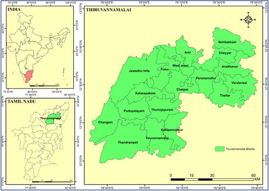
Figure 1.
Study area map for Tiruvannamalai district.
2.2. Used Data
The benefit of Synthetic Aperture Radar (SAR) is that it can collect data day or night and operates at wavelengths that are not hindered by clouds or poor lighting. With its C-SAR equipment, Copernicus Sentinel-1A can provide dependable, ongoing wide-area monitoring. Sentinel 1’s C-band imaging system features four imaging modes with various resolutions and coverage areas. It is capable of dual polarization, has a brief revisit time and delivers products quickly. For crop identification and mapping in the study area during Rabi 2020–2021, Ground Range Detected (GRD) information from Sentinel-1A Synthetic Aperture Radar image acquisition with VH polarization in interferometric wide (IW) swath mode were gathered at 12-day intervals. The data were downloaded from https://scihub.copernicus.eu/dhus/ (accessed on 10 April 2021) based on the usual peanut growing season in the research location to have complete coverage during the crop growing season, beginning 4 October 2020 to 8 January 2021.
SAR Data Processing
The multi-temporal space-borne Sentinel-1A SAR IW-GRD data were converted into terrain-geocoded values using an entirely automated processing pipeline created by [24]. The processing string was a module of the MAPscape-RICE program, created by the Swiss company Sarmap, Switzerland. The SAR time series data performed a number of important processing steps, as indicated below and as illustrated in Figure 2, to produce terrain geocoded degree values.
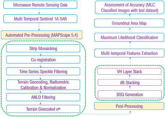
Figure 2.
Flow chart for methodology of SAR data processing and peanut area mapping.
- (i).
- Strip mosaicking: to facilitate the overall data processing and data handling,
- (ii).
- Co-registration: Images acquired with the same observation geometry were co registered in slant range geometry,
- (iii).
- Time-series speckle filtering: to balance differences in reflectivity between images,
- (iv).
- Terrain geocoding: Radiometric calibration and normalization,
- (v).
- ANLD filtering: to get smoothened homogeneous targets,
- (vi).
- Removal of atmospheric attenuation: σ° values were corrected by means of an interpolator.
- (vii).
- Subsetting: The rectangular extent of the study was extracted from the base map and the raster images were subsetted to an extent from 11°55′ to 13°15′ North latitude and 78°20′ to 79°50′ East longitude. Subsetting of raster data reduces the time in further processing.
2.3. Crop Classification and Accuracy Assessment
2.3.1. Maximum Likelihood Classification (MLC)
To classify imaging pixels into a land use/cover category based on pixel value is the purpose of the image classification process. In this work, crop area identification was performed using the maximum likelihood classification (MLC) algorithm. The spectral response pattern was used by the MLC to statistically analyze the individual categories’ variance and covariance while identifying an unidentified pixel. It was assumed that the training dataset distribution was Gaussian. According to this premise, the average vector and covariance matrix can completely represent the distribution of a training dataset for a class. The statistical possibility that a given pixel belongs to a specific class can be calculated assuming these variables.
To determine peanut, the image was first categorized using MLC with multi-temporal superimposed SAR images. Based on training pixels acquired at various locations, the training spectral signature for the peanut crop was created. The categorization for VH polarization was then completed in order to distinguish the peanut field from other categories.
2.3.2. Accuracy Assessment
The accuracy of the peanut area map was validated using the error matrix and kappa statistics. To measure the classification accuracy, each pixel’s class assignment in the classified image was contrasted with the matching class assignment on the reference data. An error matrix was created using the agreement and disagreement pixels. The elements of the matrix indicated the number of pixels in the testing dataset, while the columns and rows represented the total number of classes [25]. All of the classified output’s classification accuracy was examined.
A farmer survey was used to confirm that the observed post-harvest situation accurately reflected the presence of a peanut crop during the surveilled season. Generally, the accuracy assessment in fields was performed during the pod filling or maturity phase before harvesting, but in some cases, the field assessment was conducted during the post-season and peanut haulms. The error matrix was used to determine the accuracy metrics, including overall accuracy, producer accuracy and user accuracy [26]. The proportion of correctly identified cases located along the diagonal, which represent the overall accuracy, were determined as follows:
By dividing the total number of correctly categorized samples by the total number of reference samples, the producer’s accuracy (errors of omission) for each class was calculated as follows:
By dividing the total number of samples in a class that were verified to belong to that class by the number of samples in that class that were correctly classified, the user’s accuracy (errors of omission) of each class was calculated as follows:
2.3.3. Kappa Coefficient
The kappa coefficient, which estimates the proportionality (or percentage) increase by the classifier over a simply random assignment to classes, is a different metric for classification accuracy [27]. The formula shown below was used to estimate the kappa coefficient.
In the case of a confusion matrix containing r rows and, correspondingly, r columns:
A = the sum of r diagonal elements, which is the numerator in the computation of overall accuracy;
B = sum of the r products (row total x column total);
N = the number of pixels in the error matrix (the sum of all r individual cell values).
2.4. Crop Cutting Experiments (CCEs) for Actual Yield Estimation
The actual yield of peanut or the yield attainable by farmers during Rabi (spring) 2020–2021 was estimated with the help of the Department of Agricultural Economics and Statistics by organizing CCEs in 31 monitoring sites of Tiruvannamalai district. In each monitoring site four CCEs were organized in a randomly selected area having the size of 5 × 5 m. The average of four CCEs from each monitoring site was converted to yield (per ha) and used as the actual yield for that monitoring site. The estimated yield data were used as attainable actual yields for measuring the yield gap.
2.5. Crop Simulation Using CROPGRO Peanut Model for Potential Yield Estimation
DSSAT is a software package for microcomputers that combines crop, soil and weather information in common formats for crop modeling and application program evaluation. The DSSAT was employed in the current analysis because the user may simulate the results of cultivation techniques over a number of years for various crops in any area in the world. The elements of the crop simulation models for DSSAT are shown in Figure 3.
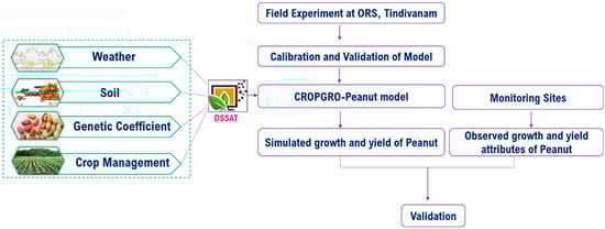
Figure 3.
Diagram of database, application and support software components in DSSAT.
In DSSAT v.4.5, the CROPGRO (crop growth) Peanut model can be utilized to simulate the daily growth and development of the peanut crop. DSSAT is a one-dimensional model that calculates daily variations in soil water content in a single layer through soil evaporation, infiltration, unsaturated flow, irrigation, vertical drainage, root water uptake and plant transpiration. In addition to crop coefficients that were thought to be less variable or even more conservative among crop cultivars, it also required cultivar coefficients (cultivar-specific characteristics) as an input to the model. The model could represent how high temperatures affected peanut development and growth. The maximum potential yield was computed using the input datasets for 31 monitoring locations by the DSSAT CROPGRO Peanut model. It needed just the small datasets mentioned for its execution.
2.5.1. Weather Data
Automatic weather stations (AWS) and regular observatories located in the study districts provided the daily meteorological information on maximum temperature (°C), minimum temperature (°C), solar radiation (MJ m−2 day−1) and rainfall (mm) for Rabi 2020–2021, which were used to create a weather file for running the CROPGRO Peanut model. To anticipate the yield, the DSSAT model needed weather information for the whole growing season of the crop.
2.5.2. Soil Data
The Department of Remote Sensing and Geographical Information Systems, Tamil Nadu Agricultural University, in Coimbatore, provided the soil data used to create the soil files. This was accomplished by using a digital soil information system that had data on the following soil parameters (1:50,000), i.e., depth; texture; pH; EC; bulk density; drainage; organic carbon; available N, P, K, Ca and Mg; and cation exchange capacity (CEC). The soil profiles’ information, as required in DSSAT, were fed into the S-Build tool in DSSAT to create a soil file. The Tiruvannamalai district comprises 12 soil series viz., Perunthurai, Devikapuram, Pedakallupalli, Meyyur, Vetavalam, Vilukam, Kolathur, Ayyalur, Perumalthangal, Mattathari, Parapperi and Kalugachalapuram, and the details were used for the S-build tool presented in Appendix A.
2.5.3. Crop Management Data
The inputs to the model for each of the 31 monitoring locations that would be simulated for Rabi 2020–2021 were documented in the crop management file (X-built) file. The actual figures of the experimental conditions and field characteristics, including the name of the weather station, the soil, initial soil water content, the field description, planting distances, the conditions of inorganic nitrogen content, irrigation and water management, fertilizer management, tillage operations, the application of organic residues and chemicals, environmental modifications, harvest management, simulation control mechanisms (specification of simulation options, i.e., starting dates, on/off options for water and nitrogen balances, symbiosis) and output options were included in the X-built tool as the crop management file.
2.5.4. Estimation of Peanut Genetic Co-Efficient
The tweaking of genetic parameters, also known as model calibration or parameterization, ensured that simulated and observed values were closely comparable. The genetic variables of cultivars were estimated using the data collected from the experiment. In order to achieve the most accurate fit between the observed and simulated number of days to the plant developmental events and grain yield at harvest, the genetic coefficients that affect the occurrence of developmental stages in the CROPGRO Peanut model entrenched in the DSSAT model were derived successively by manipulating the relevant coefficients. For developing varietal genetic coefficient, the field experiment with randomized block design was conducted for popular peanut varieties at Oilseeds Research Station, Tamil Nadu Agricultural Research Station, Tindivanam during Rabi 2019–2020 against the predominant varieties, i.e., TVM 7, TMV 13, VRI 2 and G 7 were used for generating varietal coefficient.
2.6. Yield Estimation by Integrating Remote Sensing and DSSAT CROPGRO Model
SAR Sentinel-1A data integrated with the DSSAT CROPGRO Peanut simulation model for estimating the yield are shown in Figure 4. LAI values retrieved from dB images of the SAR data were used to integrate the DSSAT simulated yield with the remote sensing data. A linear regression equation was generated between DSSAT simulated yield and spatially simulated LAI values for estimating peanut yield.
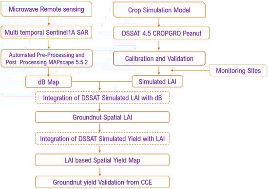
Figure 4.
Integration of remote sensing and DSSAT simulation model for yield estimation.
2.6.1. Generation of LAI for Peanut Yield Estimation
Five LAI readings were taken from each monitoring field, and the average was calculated. In order to provide information to the CROPGRO Peanut system for simulation and validation, yield data were collected at the completion of the season from each monitoring field and the entire dataset was finalized over the study area with measurements of peanut pod yield and LAI. Regression analysis was carried out between the observed and expected yield using the data from the study region pooled into a single dataset.
2.6.2. Retrieving LAI from dB Images of SAR Data
Using the point sample tool in QGIS software, v.2.18.4, the dB (back scattering) readings of peanut crops were gathered for the monitoring fields. In the monitored peanut fields of the study region, the equation for linear regression was created between the dB readings and the simulated LAI values at pod growth stage (Figure 5). The raster calculator tool in ArcMap gives users the option to create selection queries, enter map algebra syntax, or perform basic arithmetic using operators and functions. Therefore, in this investigation, the dB values of dB pictures from mature stages were substituted for the calculated regression values using the raster calculator in ArcMap. To construct yield maps and statistics spatially, an empirical method was used to extrapolate the field observed and DSSAT calculated LAI values (Figure 6).
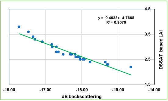
Figure 5.
Integration of DSSAT simulated LAI and maximum SAR dB backscattering at pod formation stage.
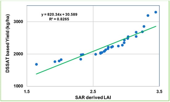
Figure 6.
Integration of SAR derived LAI and DSSAT simulated yield for the estimation of spatial variability.
2.7. Yield Gap Estimation
Yield gap is defined as the difference between potential yield (Yp) and average yield (Ya). The potential yield was derived from the crop simulation model CROPGRO Peanut by a trail conducted at Oilseeds Research Station, Tindivanam. The basic information essential for DSSAT model calibration and validation were used from this trial and allowed to estimate the potential yield of peanut for the study area. The actual yield data of peanut were collected by organizing the crop cutting experiments (CCEs) in the study area.
3. Results and Discussion
3.1. Peanut Area and Accuracy Assessment
The peanut area map for the Tiruvannamalai district was derived from multi-temporal C-band SAR imagery of the Sentinel-1A satellite. Using the shape files of administrative boundaries, the map of the district and blocks and statistics of the peanut area were extracted for 18 blocks of Tiruvannamalai district. The classified peanut area for each block is shown in Table 1 and Figure 7 and the total peanut growing area during the Rabi (spring) 2020–2021 was estimated to be 32,298 ha. The Thandrampet block of Tiruvannamalai district had the maximum area, with 6970 ha, followed by the Thurinjapuram, Tiruvannamalai, Keelpennathur and Chengam blocks, which had 5576, 5197, 4989 and 4111 ha, respectively. The Jawadhu hills block of Tiruvannamalai district recorded a minimum area of 29 ha.

Table 1.
Peanut area divided in blocks for the Tiruvannamalai district of Tamil Nadu during Rabi 2020–2021.
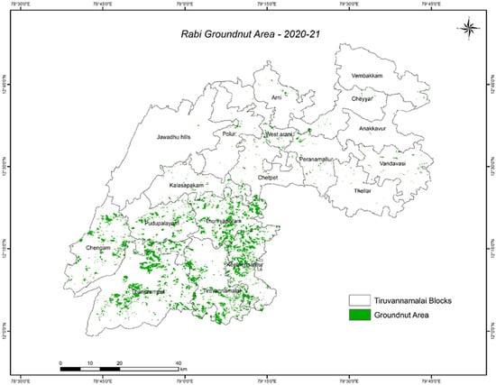
Figure 7.
Peanut area of Tiruvannamalai district during Rabi 2020–2021.
The peanut area maps were assessed for accuracy on a peanut or non-peanut basis, where all other land cover types were grouped into a non-peanut class. In total 103 validation points, of which there were 69 peanut and 34 non-peanut points, were considered for validation and the confusion matrix is shown in Table 2. The overall classification accuracy was 87.4% with a kappa score of 0.75, indicating the accuracy of classification. The overall accuracy (>80%) and kappa score (>0.50) indicated that the assessment was of high quality. The results were in accordance with [28,29,30,31], who delineated the crop area estimation with high classification accuracy using multi-temporal Sentinel-1A data; this indicated the suitability of remote-sensing-based images for crop area estimation and monitoring for policy decisions, including crop insurance.
Table 2.
Confusion matrix for accuracy assessment for peanut classification during Rabi 2020–2021.
3.2. Genetic Coefficient Development and Calibration of DSSAT Model
Crop simulation model genetic coefficient development and calibration are vital for establishing their credibility and ability in simulating growth, development, production quality and yield [32]. Among the four varietal genetic coefficients (Table 3) generated during the Rabi season 2019–2020, the time between emergence to flower appearance (EM-FL) and the time between the first flower to first pod (FL-SH) ranged from 17.50 to 19.00 photothermal days and from 7.00 to 8.00 ones, respectively. In contrast, the time between the first flower and the first seed (FL-SD) and the time between the first seed and the physiological maturity stage (SD-PM) ranged from 17.30 to 18.50 photothermal days and from 58.00 to 62.00 ones, respectively. The maximum leaf photosynthesis rate ranged from 1.09 to 1.25 mg CO2 m−2 s−1. The seed filling duration (SFDUR) ranged from 31 to 33 photothermal days, while the amount of seeds per pod was 1.65, for six varieties. Similarly, Refs. [33,34,35,36] developed genetic coefficient for groundnut cultivars to various agro-climatic zones of India, for crop yield estimation using simulation models.
Table 3.
Developed genetic coefficient for predominant varieties of peanut in the Tiruvannamalai district of Tamil Nadu.
The capability of the DSSAT CROPGRO Peanut model to predict growth and development of the four predominant peanut cultivars, i.e., TMV7, TMV13, VRI 2 and G7 (Table 4) were assessed; the crop response was predicted as influenced by season, weather, management and soil distribution through field experiments conducted at Oilseeds Research Station, Tindivanam.
Table 4.
Growth and development variables simulated by DSSAT CROPGRO Peanut on predominant varieties cultivated in the study area.
Further, the DSSAT model allowed researchers to record a simulated canopy height from 56 to 69 cm, as well as the maximum LAI for these six varieties ranging from 4.93 to 5.60. These simulation results were in line with those of [37], who deduced that when independent crop and soil datasets were used for evaluation, the PNUTGRO model was influenced by season and location for simulating growth and crop yield. Apart from that, Refs. [38,39,40] tried to simulate the varietal influence on the growth and physiological process at different regions using DSSAT crop simulation model. The simulated pod yield of different peanut varieties ranged from 3935 to 4657 kg ha−1. The results obtained in this study among the varieties highly correlated with those achieved by [28], who simulated the potential yield of rainfed peanut in the major production zones of Tamil Nadu, which correlated highly with the results obtained in the present study among the varieties. Similar findings on pod yield simulation by DSSAT in a different location were reported by [36,37,41,42,43], and the simulation model overestimated the pod yield rather than the attainable actual yield, because its simulation of crops had simulated the yield without considering the limiting factors. The CROPGRO Peanut model was used by [34] to simulate the phenological events, yield and production quality of peanut cultivars, i.e., GG 2 and GG 20, in Gujarat. In the past years, many research efforts were carried out to simulate the growth and productivity of peanut and other crops.
3.3. Spatial Estimation of Potential Yield, Actual Yield and Yield Gap of Peanut
3.3.1. Potential Yield Estimation
The DSSAT simulation model allowed researchers to estimate the peanut potential yield in the monitoring sites, divided into blocks, in Tiruvannamalai district (Table 5 and Table 6). According to [44]’s regression analysis, DSSAT is a useful method for creating yield prediction models. Among the monitoring sites, the maximum potential yield of 4843 kg/ha was simulated using CROPGRO Peanut at Mel Palur and Kil Palur villages, while the minimum potential yield of 3194 kg/ha was simulated at Tandarai village of Tiruvannamalai district. Similarly, from the potential yield of 18 blocks of Tiruvannamalai district, the minimum potential yield varied from 3711 to 3821 kg/ha, recorded at the Pernamallur and Jawadhu hills blocks, respectively, with a mean minimum yield of 3750 kg/ha. The maximum potential yield varied from 3936 to 4306 kg/ha, recorded in the Vembakkam and Thandarampet blocks, respectively, with the mean maximum yield of 4029 kg/ha. The mean overall potential yield of Tiruvannamalai district was 3874 kg/ha and the potential yield map is shown in Figure 8.
Table 5.
Peanut potential, actual yield and yield gap estimated for monitoring sites of the Tiruvannamalai district of Tamil Nadu during Rabi 2020–2021.
Table 6.
Spatial variability of peanut potential yield, actual yield and yield gap estimated for the Tiruvannamalai district of Tamil Nadu during Rabi 2020–2021.
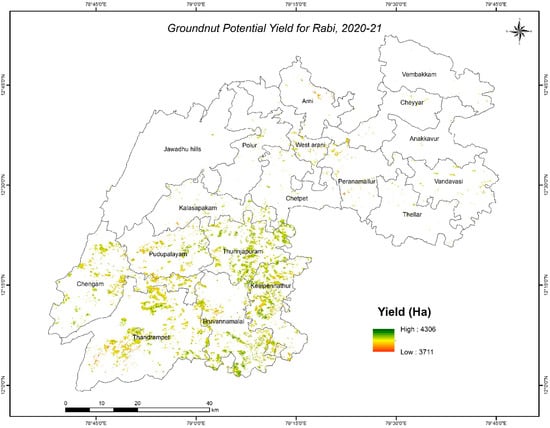
Figure 8.
Peanut potential yield of Tiruvannamalai district during Rabi 2020–2021.
As the DSSAT simulation model is based on the optimum input data of soil, water, climate and crop management, the potential yield estimation always provides a yield higher than the yield attainable by farmers, similarly to the results of other scientists [45]. The DSSAT model simulates daily leaf area index (LAI), vegetation status parameters, biomass production and potential yield, using soil, crop management and daily weather data as inputs.
Moreover, simulation models provide the most accurate estimate of potential yield, because they account for temporal (during the years) and spatial (in the regions) variability of weather parameters, as well as the major interactions among crops, weather, soil, water regime and crop management. They allow quantification of the potential or water-limited yield within the climatic, soil and management context of a given cropping system. Hence, if it is possible to use the spatial and temporal variability of the above parameters, crop simulation models will perform much better than empirical methods [5].
3.3.2. Actual Yield Estimation
Crop cutting experiments (CCEs) allowed estimations of the actual yield of monitoring sites, divided into blocks; the results are shown in Table 5 and Table 6. Actual peanut yields recorded in monitoring locations of the Tiruvannamalai district during the Rabi 2020–2021 ranged from 1228 to 3106 kg/ha in the Agaramand and Mel Palur villages, respectively. Among the blocks of Tiruvannamalai district, the minimum actual yields were from 1394 to 1644 kg/ha in the Tandarampet and Jawadhu hills blocks, while the maximum yields ranged from 1858 to 2526 kg/ha in the Vembakkam and Tandarampet blocks, respectively. The mean overall actual yield was 1740 kg/ha and the actual yield map is shown in Figure 9.
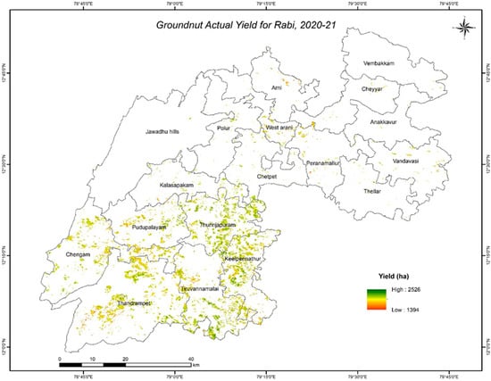
Figure 9.
Spatial peanut actual yield of Tiruvannamalai district during Rabi 2020–2021.
During the Rabi 2020–2021, the actual crop yield decreased compared with the previous years. However, such a decrease in the actual yield was accompanied by a significant fluctuation from year to year, maybe due to rainfall variability. According to [46], there is a correlation between the growing season rainfall and the annual actual yield. The decrease in actual yield could be the result of changes in agronomic practices adopted in the region during the considered period, although this decrease was found at its early stage.
3.3.3. Peanut Yield Gap Estimation
The yield gap of monitoring sites and the spatial variability of yield gap in the various blocks are shown in Table 5 and Table 6. Among the monitoring sites, Ponnaiyur village recorded the maximum yield gap of 2346 kg/ha, whereas Mangalam village recorded the minimum yield gap of 1217 kg/ha, compared with other monitoring sites. For the Tiruvannamalai district, the minimum yield gap ranged from 1456 to 2072 kg/ha in the Tiruvannamalai and Vembakkam blocks, while the maximum yield gap from 2231 to 2508 kg/ha was recorded in the Thellar and Tiruvannamalai blocks, respectively. The mean overall yield gap of Tiruvannamalai district was 2134 kg/ha. By combining remote sensing (from SAR Sentinel-1A satellite) data with those obtained by means of the crop simulation model (DSSAT CROPGRO Peanut), the yield gap of peanut was investigated in this work for Rabi 2020–2021; the yield gap map is shown in Figure 10. The yield gap ranged from 1217 to 2346 kg/ha and the major production constraints of peanut in the district were seasonal rainfall variability, poor soil fertility, lack of improved varieties and inadequate weed management. The current yield gap could be minimized by combining traditional agronomic approaches with the latest technologies, as well as by involving different stakeholders. A substantial amount of work was devoted to mapping and interpreting the within-field spatial variability of yield, in order to perform spatially variable rate application of crop inputs, according to the principles of precision agriculture [4].
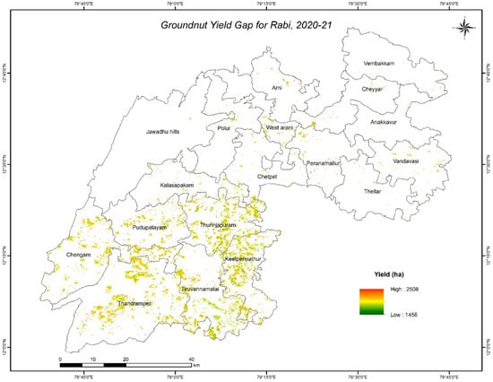
Figure 10.
Peanut yield gap for Tiruvannamalai district during Rabi 2020–2021.
4. Conclusions
The integration of SAR Sentinel-1A with DSSAT CROPGRO Peanut for assessing the peanut yield gap during the Rabi 2020–2021 in Tiruvannamalai district recorded an average yield gap of 2134 kg/ha, with a mean minimum gap of 1890 kg/ha and a maximum gap of 2324 kg/ha. The key production constraints of the peanut growing areas in Tamil Nadu were seasonal rainfall unpredictability, poor soil fertility, lack of improved varieties and inadequate weed management, which created a wide gap between the potential and attainable yields. The current yield gap could be minimized by combining traditional agronomic approaches with the latest technologies, as well as by involving different stakeholders. As a result, the regular use of remote sensing for examining the magnitude and the causes of yield gap and, then, improving the awareness of the yield gap itself will be critical in satisfying future crop demand at reasonable prices, while minimizing the environmental impact.
Author Contributions
All the authors (S.T., S.P., N.S.S., K.R., R.K. and R.M.) contributed substantially to this manuscript. Conceptualization, S.P.; methodology, K.R. and R.K.; validation, S.T. and N.S.S.; formal analysis, S.T. and N.S.S.; investigation, S.P., K.R. and R.K.; writing—original draft preparation, S.T., N.S.S. and G.S.; writing—review and editing, S.P., K.R., R.K. and R.M.; supervision, S.P. and K.R.; funding acquisition, S.P., K.R. and R.K. All authors have read and agreed to the published version of the manuscript.
Funding
This research received no external funding.
Institutional Review Board Statement
Not applicable.
Informed Consent Statement
Not applicable.
Data Availability Statement
Not applicable.
Acknowledgments
The authors acknowledge the Agriculture and Land Eco system Division, Space Application Centre, ISRO, Ahmedabad for providing the funding to carry out the investigation work in a project mode (Space Technology Utilization for Food Security, Agricultural Assessment and Monitoring—SUFALAM Project). They also acknowledge the Professor and Head of Staff of the Department of Remote Sensing and GIS, TNAU for their invaluable assistance, comments and constructive suggestions on the research and manuscript. We would also like to thank everyone who provided technical assistance during the study’s execution.
Conflicts of Interest
The authors declare no conflict of interest.
Appendix A
Table A1.
Predominant soil series information of Tiruvannamalai district used in S-built tool of DSSAT model.
Table A1.
Predominant soil series information of Tiruvannamalai district used in S-built tool of DSSAT model.
| Soil Series | Depth | Sand (%) | Silt (%) | Clay (%) | Texture Class | pH | EC | OC (%) | CEC | ESP |
|---|---|---|---|---|---|---|---|---|---|---|
| Perundurai | 13 | 79.00 | 6.00 | 15.00 | Sandy loam | 6.00 | 0.25 | 0.41 | 10.60 | 2.74 |
| 38 | 41.00 | 11.00 | 48.00 | Clay | 5.90 | 0.22 | 0.50 | 22.80 | 1.32 | |
| 70 | 23.00 | 8.00 | 69.00 | Clay | 5.90 | 0.18 | 0.70 | 26.40 | 1.52 | |
| 92 | 45.00 | 9.00 | 46.00 | Clay | 6.40 | 0.18 | 0.30 | 19.20 | 1.61 | |
| Devikapuram | 14 | 43.80 | 21.60 | 34.60 | Clay loam | 7.00 | 0.10 | 0.52 | 14.51 | 0.76 |
| 44 | 65.80 | 12.30 | 21.90 | Sandy clay loam | 7.30 | 0.10 | 0.17 | 10.23 | 0.88 | |
| 59 | 64.90 | 12.80 | 22.30 | Sandy clay loam | 7.40 | 0.10 | 0.23 | 11.12 | 1.08 | |
| 79 | 66.30 | 16.90 | 16.80 | Sandy loam | 7.70 | 0.10 | 0.11 | 8.64 | 0.69 | |
| 98 | 68.70 | 7.50 | 23.80 | Sandy clay loam | 7.50 | 0.10 | 0.20 | 12.46 | 0.56 | |
| Meyyur | 16 | 51.02 | 25.17 | 23.81 | Sandy clay loam | 8.90 | 0.40 | 0.75 | 39.53 | 1.10 |
| 30 | 36.27 | 32.90 | 30.83 | Clay loam | 9.00 | 0.70 | 0.78 | 40.32 | 1.08 | |
| 50 | 20.21 | 35.67 | 44.12 | Clay | 9.30 | 1.10 | 0.80 | 42.84 | 1.02 | |
| 110 | 42.39 | 11.49 | 46.12 | Clay | 9.10 | 0.90 | 0.65 | 42.00 | 1.04 | |
| Vetavalam | 25 | 65.12 | 15.68 | 19.20 | Sandy clay loam | 7.20 | 0.40 | 0.64 | 21.94 | 1.19 |
| 52 | 73.54 | 12.26 | 14.20 | Sandy loam | 6.90 | 0.30 | 0.67 | 21.41 | 1.21 | |
| Villukam | 14 | 46.72 | 18.28 | 35.00 | Clay | 8.50 | 1.41 | 0.31 | 27.10 | 2.80 |
| 36 | 44.41 | 18.89 | 36.70 | Clay | 7.90 | 0.25 | 0.32 | 28.20 | 1.38 | |
| 72 | 42.11 | 19.00 | 38.89 | Clay | 7.80 | 0.22 | 0.30 | 30.10 | 1.40 | |
| 103 | 37.34 | 22.66 | 40.00 | Clay | 7.80 | 0.20 | 0.25 | 31.26 | 1.02 | |
| Kollattur | 18 | 64.77 | 14.34 | 20.89 | Sandy clay loam | 6.34 | 0.05 | 0.45 | 11.40 | 4.91 |
| 47 | 56.37 | 3.95 | 39.68 | Sandy clay | 6.69 | 0.04 | 0.37 | 13.80 | 2.90 | |
| Ayyalur | 16 | 87.10 | 8.00 | 4.90 | Loamy sand | 6.60 | 0.02 | 0.32 | 10.60 | 2.08 |
| 40 | 43.00 | 17.00 | 40.00 | Clay loam | 6.20 | 0.22 | 0.17 | 15.40 | 1.43 | |
| 75 | 60.36 | 2.29 | 37.35 | Sandy clay | 6.50 | 0.20 | 0.28 | 24.80 | 0.97 | |
| 127 | 59.90 | 2.60 | 37.50 | Sandy clay | 6.60 | 0.10 | 0.17 | 21.95 | 1.23 | |
| Perumaltangal | 14 | 40.26 | 23.46 | 36.28 | Clay | 7.17 | 0.16 | 0.56 | 22.00 | 5.83 |
| 51 | 34.89 | 24.87 | 40.24 | Clay | 7.27 | 0.13 | 0.41 | 25.60 | 4.88 | |
| Matathari | 12 | 12.30 | 43.20 | 44.50 | Silty clay | 8.60 | 0.30 | 0.54 | 23.00 | 12.61 |
| 25 | 9.30 | 44.40 | 46.30 | Silty clay | 8.50 | 0.30 | 0.43 | 23.24 | 8.18 | |
| 55 | 53.20 | 8.50 | 38.30 | Sandy clay | 8.50 | 0.20 | 0.38 | 28.00 | 6.43 | |
| 85 | 51.80 | 10.60 | 37.60 | Sandy clay | 8.50 | 0.20 | 0.34 | 30.24 | 5.62 | |
| Papperi | 12 | 66.00 | 13.20 | 20.80 | Sandy clay loam | 7.00 | 0.30 | 0.30 | 7.80 | 25.64 |
| 23 | 67.50 | 10.90 | 21.60 | Sandy clay loam | 7.00 | 0.20 | 0.20 | 8.80 | 11.36 | |
| 40 | 66.40 | 11.20 | 22.40 | Sandy clay loam | 7.30 | 0.20 | 0.20 | 7.22 | 24.93 | |
| 85 | 67.20 | 11.00 | 21.80 | Sandy clay loam | 7.30 | 0.20 | 0.20 | 6.22 | 25.72 | |
| Kalugachalapuram | 12 | 35.00 | 22.00 | 43.00 | Clay | 6.44 | 0.52 | 0.84 | 19.60 | 5.61 |
| 35 | 34.00 | 20.00 | 46.00 | Clay | 6.55 | 0.44 | 0.62 | 22.30 | 7.17 | |
| 68 | 32.00 | 19.00 | 49.00 | Clay | 6.59 | 0.53 | 0.60 | 22.60 | 5.84 | |
| 86 | 24.60 | 24.80 | 50.60 | Clay | 6.56 | 0.69 | 0.58 | 27.80 | 4.53 | |
| 113 | 24.40 | 29.60 | 46.00 | Clay | 6.40 | 0.50 | 0.52 | 28.50 | 3.51 |
References
- Chapagain, T.; Good, A. Yield and production gaps in rainfed wheat, barley, and canola in Alberta. Front. Plant Sci. 2015, 6, 990–999. [Google Scholar] [CrossRef]
- Hochman, Z.; Gobbett, D.; Horan, H.; Garcia, F.J.N. Data rich yield gap analysis of wheat in Australia. Field Crop. Res. 2016, 197, 97–106. [Google Scholar] [CrossRef]
- Eash, L.; Fonte, S.J.; Sonder, K.; Honsdorf, N.; Schmidt, A.; Govaerts, B.; Verhulst, N. Factors contributing to maize and bean yield gaps in Central America vary with site and agroecological conditions. J. Agric. Sci. 2017, 157, 300–317. [Google Scholar] [CrossRef]
- Lobell, D.B.; Cassman, K.G.; Field, C.B. Crop yield gaps: Their importance, magnitudes, and causes. Annu. Rev. Environ. Resour. 2009, 34, 179–204. [Google Scholar] [CrossRef]
- Van Ittersum, M.; Cassman, K.G.; Grassini, P.; Wolf, J.; Tittonell, P.; Hochman, Z. Yield gap analysis with local to global relevance—A review. Field Crop. Res. 2013, 143, 4–17. [Google Scholar] [CrossRef]
- Cassman, K. What do we need to know about global food security? Glob. Food Secur. 2012, 1, 81–82. [Google Scholar] [CrossRef]
- Najafi, E.; Devineni, N.; Khanbilvardi, R.M.; Kogan, F. Understanding the changes in global crop yields through changes in climate and technology. Earth’s Future 2016, 6, 410–427. [Google Scholar] [CrossRef]
- Soltani, A.; Alimagham, S.M.; Nehbandani, A.; Torabi, B.; Zeinali, E.; Zand, E.; Vadez, V.D.; Van Loon, M.P.; Van Ittersum, M.K. Future food self-sufficiency in Iran: A model-based analysis. Glob. Food Secur. 2020, 24, 100351–100359. [Google Scholar] [CrossRef]
- Laborte, A.G.; de Bie, K.; Smalinga, E.M.A.; Moya, P.F.; Boling, A.A.; Van Ittersum, M.K. Rice yields and yield gaps in Southeast Asia: Past trends and future outlook rice yields and yield gaps in Southeast Asia: Past trends and future outlook. Eur. J. Agron. 2012, 36, 9–20. [Google Scholar] [CrossRef]
- FAO; DWFI. Yield Gap Analysis of Field Crops—Methods and Case Studies; Sadras, V.O., Cassman, K.G.G., Grassini, P., Hall, A.J., Bastiaanssen, W.G.M., Laborte, A.G., Milne, A.E., Sileshi, G., Steduto, P., Eds.; FAO Water Reports No. 41; FAO: Rome, Italy, 2015. [Google Scholar]
- Paul, G.C.; Saha, S.; Hembram, T.K. Application of phenology-based algorithm and linear regression model for estimating rice cultivated areas and yield using remote sensing data in Bansloi River Basin, Eastern India. Remote Sens. Appl. Soc. Environ. 2020, 19, 100367. [Google Scholar]
- Deka, R.L.; Hussain, R.; Singh, K.K.; Rao, V.U.M.; Balasubramaniyam, R.; Baxla, A.; Rao, V.; Balasubramaniyam, R. Rice phenology and growth simulation using CERES-rice model under the agro-climate of upper brahmaputra valley of Assam. Mausam 2016, 67, 591–598. [Google Scholar] [CrossRef]
- Dwivedi, M.; Saxena, S.; Ray, S.S. Assessment of rice biomass production and yield using semi-physical approach and remotely sensed data. Int. Arch. Photogramm. Remote Sens. Spat. Inf. Sci. 2019, 42, 217–222. [Google Scholar]
- Lobell, D.B. The use of satellite data for crop yield gap analysis. Field Crop. Res. 2013, 143, 56–64. [Google Scholar] [CrossRef]
- Soltani, A.; Sinclair, T.R. Modeling Physiology of Crop Development, Growth and Yield; CABI: Oxfordshire, UK; Cambridge, MA, USA, 2012. [Google Scholar]
- Eitzinger, J.; Thaler, S.; Schmid, E.; Strauss, F.; Ferrise, R.; Moriondo, M.; Bindi, M.; Palosuo, T.; Rötter, R.; Kersebaum, K.C.; et al. Sensitivities of crop models to extreme weather conditions during flowering period demonstrated for maize and winter wheat in Austria. J. Agric. Sci. 2013, 151, 813–835. [Google Scholar] [CrossRef]
- Batchelor, W.D.; Basso, B.; Paz, J.O. Examples of strategies to analyze spatial and temporal yield variability using crop models. Eur. J. Agron. 2002, 18, 141–158. [Google Scholar] [CrossRef]
- Xie, Y.; Sha, Z.; Yu, M. Remote sensing imagery in vegetation mapping: A review. J. Plant Ecol. 2008, 1, 9–23. [Google Scholar] [CrossRef]
- Burke, M.; Lobell, D.B. Satellite-Based Assessment of Yield Variation and Its Determinants in Smallholder African Systems. Proc. Natl. Acad. Sci. USA 2017, 114, 2189–2194. [Google Scholar] [CrossRef]
- Inoue, Y. Synergy of remote sensing and modeling for estimating ecophysiological processes in plant production. Plant Prod. Sci. 2003, 6, 3–16. [Google Scholar] [CrossRef]
- Dorigo, W.A.; Zurita-Milla, R.; de Wit, A.J.W.; Brazile, J.; Singh, R.; Schaepman, M.E. A review on reflective remote sensing and data assimilation techniques for enhanced agroecosystem modeling. Int. J. Appl. Earth Obs. Geoinf. 2007, 9, 165–193. [Google Scholar] [CrossRef]
- Adhikari, K.; Carre, F.; Toth, G. Site-Specific Land Management General Concepts and Applications; European Commission: Luxembourg, 2009. [Google Scholar]
- Venkatesan, M.; Pazhanivelan, S. Estimation of Maize Yield at Spatial Level Using DSSAT Crop Simulation Model. Madras Agric. J. 2018, 1, 105–115. [Google Scholar] [CrossRef]
- Holecz, F.; Barbieri, M.; Collivignarelli, F.; Gatti, L.; Nelson, A.; Setiyono, T.D.; Boschetti, M.; Manfron, G.; Brivio, P.A.; Quilang, J.E.; et al. An operational remote sensing based service for rice production estimation at national scale. In Proceedings of the Living Planet Symposium, Edinburgh, UK, 9–13 September 2013. [Google Scholar]
- Lillesand, T.M. Strategies for improving the accuracy and specificity of large-area, satellite-based land cover inventories. Int. Arch. Photogramm. Remote Sens. 1994, 30, 23–30. [Google Scholar]
- Congalton, R.G. A review of assessing the accuracy of classifications of remotely sensed data. Remote Sens. Environ. 1991, 37, 35–46. [Google Scholar] [CrossRef]
- Richards, J.A. Sources and characteristics of remote sensing image data. In Remote Sensing Digital Image Analysis; Springer: Berlin, Germany, 1993; pp. 1–37. [Google Scholar]
- Deiveegan, M.; Pazhanivelan, S.; Ragunath, K.; Kumaraperumal, R. Detection of Agricultural Vulnerability to Drought Using NDVI and Land Surface Temperature in Salem and Namakkal districts of Tamil Nadu. Adv. Life Sci. 2016, 5, 6868–6873. [Google Scholar]
- Venkatesan, M.; Pazhanivelan, S.; Sudarmanian, N.S. Multi-Temporal Feature Extraction for Precise Maize Area Mapping Using Time-Series Sentinel 1A SAR Data. Int. Arch. Photogramm. Remote Sens. Spat. Inf. Sci. 2019, XLII-3/W6, 169–173. [Google Scholar] [CrossRef]
- Sudarmanian, N.S.; Pazhanivelan, S.; Ragunath, K.; Panneerselvam, S. Estimation of methane emission from rice fields using satellite data in Thiruvarur district. Madral Agric. J. 2019, 7, 4116–4120. [Google Scholar]
- Pazhanivelan, S.; Geethalakshmi, V.; Tamilmounika, R.; Sudarmanian, N.S.; Kaliaperumal, R.; Ramalingam, K.; Sivamurugan, A.P.; Mrunalini, K.; Yadav, M.K.; Quicho, E.D. Spatial Rice Yield Estimation Using Multiple Linear Regression Analysis, Semi-Physical Approach and Assimilating SAR Satellite Derived Products with DSSAT Crop Simulation Model. Agronomy 2022, 12, 2008. [Google Scholar] [CrossRef]
- Chisanga, C.B.; Phiri, E.; Chinene, V. Evaluating APSIM-and-DSSAT-CERES-Maize Models under Rainfed Conditions Using Zambian Rainfed Maize Cultivars. Nitrogen 2021, 2, 392–414. [Google Scholar] [CrossRef]
- Yadav, S.; Patel, H.; Patel, G.; Lunagaria, M.; Karande, B.; Shah, A.; Pandey, V. Calibration and validation of PNUTGRO (DSSATv4.5) model for yield and yield attributing characters of kharif Peanut cultivars in middle Gujarat region. J. Agrometeorol. 2012, 14, 24–29. [Google Scholar]
- Parmar, P.; Patel, H.; Yadav, S.; Pandey, V. Calibration and validation of DSSAT model for kharif Peanut in North-Saurashtra agro-climatic zone of Gujarat. J. Agrometeorol. 2013, 15, 62. [Google Scholar] [CrossRef]
- Naab, J.; Boote, K.; Jones, J.; Porter, C. Adapting and evaluating the CROPGRO-peanut model for response to phosphorus on a sandy-loam soil under semi-arid tropical conditions. Field Crop. Res. 2015, 176, 71–86. [Google Scholar] [CrossRef]
- Halder, D.; Panda, R.; Srivastava, R.; Kheroar, S. Evaluation of the CROPGRO-Peanut model in simulating appropriate sowing date and phosphorus fertilizer application rate for peanut in a subtropical region of eastern India. Crop J. 2017, 5, 317–325. [Google Scholar] [CrossRef]
- Gilbert, R.; Boote, K.; Bennett, J. On-farm testing of the PNUTGRO crop growth model in Florida. Peanut Sci. 2002, 29, 58–65. [Google Scholar] [CrossRef]
- Pandey, V.; Shekh, A.; Vadodaria, R.; Bhatt, B. Evaluation of CROPGRO peanut model for two genotypes under different environment. In National Seminar on Agro Meteorological Research for Sustainable Agricultural Production at GAU Anand; Association of Agrometeorologists: Anand, India, 2001. [Google Scholar]
- Garcia, A.G.; Hoogenboom, G.; Guerra, L.; Paz, J.; Fraisse, C. Analysis of the inter-annual variation of peanut yield in Georgia using a dynamic crop simulation model. Trans. ASABE 2006, 49, 2005–2015. [Google Scholar] [CrossRef]
- Biswal, A.; Sahay, B.; Ramana, K.; Rao, S.; Sai, M. Relationship between AWiFS derived Spectral Vegetation Indices with Simulated Wheat Yield Attributes in Sirsa district of Haryana. Int. Arch. Photogramm. Remote Sens. Spat. Inf. Sci. 2014, 40, 689. [Google Scholar] [CrossRef]
- Bhatia, V.; Singh, P.; Wani, S.; Srinivas, K. Yield gap analysis of Peanut in India using simulation modeling. Glob. Theme Agro Ecosyst. Rep. 2005, 43. Available online: https://www.iwmi.cgiar.org/assessment/files_new/publications/ICRISATReportNo_31 (accessed on 10 April 2022).
- Anothai, J.; Patanothai, A.; Pannangpetch, K.; Jogloy, S.; Boote, K.; Hoogenboom, G. Multi-environment evaluation of peanut lines by model simulation with the cultivar coefficients derived from a reduced set of observed field data. Field Crop. Res. 2009, 110, 111–122. [Google Scholar] [CrossRef]
- Putto, C.; Patanothai, A.; Jogloy, S.; Pannangpetch, K.; Boote, K.; Hoogenboom, G. Determination of efficient test sites for evaluation of peanut breeding lines using the CSM-CROPGRO-peanut model. Field Crop. Res. 2009, 110, 272–281. [Google Scholar] [CrossRef]
- Maloom, J.M.; Saludes, R.B.; Dorado, M.A.; Cruz, P.C.S. Development of a GIS-Based Model for Predicting Rice Yield. Philipp. J. Crop Sci. 2014, 39, 8–19. [Google Scholar]
- Hoogenboom, G.; Porter, C.H.; Boote, K.J.; Shelia, V.; Wilkens, P.W.; Singh, U.; White, J.W.; Asseng, S.; Lizaso, J.I.; Moreno, L.P.; et al. The DSSAT crop modeling ecosystem. In Advances in Crop Modeling for a Sustainable Agriculture; Boote, K.J., Ed.; Burleigh Dodds Science Publishing: Cambridge, UK, 2019; pp. 173–216. [Google Scholar]
- Shiferaw, W.; Yoseph, T. Collection, characterization and evaluation of sorghum (Sorghum bicolor (L.) Moench) landraces from South Omo and Segen people’s zone of South Nation Nationality Peoples Region, Ethiopia. Int. Res. J. Agric. Sci. Soil Sci. 2014, 4, 76–84. [Google Scholar]


Disclaimer/Publisher’s Note: The statements, opinions and data contained in all publications are solely those of the individual author(s) and contributor(s) and not of MDPI and/or the editor(s). MDPI and/or the editor(s) disclaim responsibility for any injury to people or property resulting from any ideas, methods, instructions or products referred to in the content. |
© 2023 by the authors. Licensee MDPI, Basel, Switzerland. This article is an open access article distributed under the terms and conditions of the Creative Commons Attribution (CC BY) license (https://creativecommons.org/licenses/by/4.0/).