Research on Winter Jujube Object Detection Based on Optimized Yolov5s

Abstract

Winter jujube is a popular fresh fruit in China for its high vitamin C nutritional value and delicious taste. In terms of winter jujube object detection, in machine learning research, small size jujube fruits could not be detected with a high accuracy. Moreover, in deep learning research, due to the large model size of the network and slow detection speed, deployment in embedded devices is limited. In this study, an improved Yolov5s (You Only Look Once version 5 small model) algorithm was proposed in order to achieve quick and precise detection. In the improved Yolov5s algorithm, we decreased the model size and network parameters by reducing the backbone network size of Yolov5s to improve the detection speed. Yolov5s’s neck was replaced with slim-neck, which uses Ghost-Shuffle Convolution (GSConv) and one-time aggregation cross stage partial network module (VoV-GSCSP) to lessen computational and network complexity while maintaining adequate accuracy. Finally, knowledge distillation was used to optimize the improved Yolov5s model to increase generalization and boost overall performance. Experimental results showed that the accuracy of the optimized Yolov5s model outperformed Yolov5s in terms of occlusion and small target fruit discrimination, as well as overall performance. Compared to Yolov5s, the Precision, Recall, mAP (mean average Precision), and F₁ values of the optimized Yolov5s model were increased by 4.70%, 1.30%, 1.90%, and 2.90%, respectively. The Model size and Parameters were both reduced significantly by 86.09% and 88.77%, respectively. The experiment results prove that the model that was optimized from Yolov5s can provide a real time and high accuracy small winter jujube fruit detection method for robot harvesting.

1. Introduction

Winter jujube is a popular fresh fruit in China for its high vitamin C nutritional value and delicious taste. The fruit maturity on the same jujube tree varies greatly due to the long ripening period of the winter jujube, and the fruit-picking process is primarily manual. The labor input needed for the picking process represents 40% of the total labor demand in the orchard production chain [1]. Manual picking is time-consuming, ineffective, and expensive. Research on winter jujube picking robots is essential in order to lower picking costs and labor intensity.

One of the key technologies of the winter jujube picking robot is the quick identification and localization of winter jujube fruits. The use of machine learning for image processing is a hot research topic. For machine vision systems, machine learning can be divided into supervised learning and unsupervised learning, depending on whether the input data are labeled or not. Target detection networks such as the You only look once (Yolo) series belong to supervised learning algorithms that require the input of labeled samples. For unlabeled input samples, unsupervised learning algorithms such as k-means and Gaussian mixture models are utilized. DetCo [2] is an unsupervised target detection algorithm that learns a discriminative representation for target detection by contrasting loss between global image and local image blocks. However, its hierarchical intermediate loss of contrast adds significant computing time, which does not meet the real-time detection requirements. Thus, unsupervised learning is usually not directly used for real-time target detection tasks.

Target detection has significantly improved in various fields due to the recent rapid advancement of deep learning techniques. These fields include medical disease diagnosis [3,4,5], fruit quality inspection [6], and industrial defect detection [7]. Target detection is also extensively used in the agricultural industry, such as in the identification of apple leaf diseases [8], location of banana bunches and stalks [9], and tomato classification [10]. The success of these applications serves as a reference for winter jujube target detection.

Because of AlexNet’s success in the recognition of visible images, deep learning was introduced and quickly developed in the field of computer vision [11]. Networks such as Visual Geometry Group (VGG) Net [12] and GoogLeNet [13] were subsequently suggested one after the other. Fully Convolutional Networks (FCN), which do away with Convolutional Neural Networks (CNN) fully connected layer and define a leapfrog architecture, were proposed by Jonathan Long et al. [14] in 2015. The primary innovation of this architecture was the successful blending of appearance information from shallow and fine layers with semantic information from deep and coarse layers. In light of this, Williams et al. [15] created a novel multi-arm kiwi-harvesting robot with a vision system that made use of FCN networks and stereo matching algorithms for the accurate detection and localization of kiwi fruit in natural lighting. Deep learning-based target detection algorithms have made significant progress in recent years, and two categories of algorithms with excellent detection performance and wide adoption can be identified. R-CNN [16], Fast R-CNN [17], and Faster R-CNN [18] are examples of the R-CNN series algorithm based on region proposals. These two-stage algorithms require heuristic methods (selective search) or the Region Proposal Network (RPN) to generate region proposals first before performing classification and regression on those proposals. The Yolo series [19,20,21] of one-stage algorithms is the second class of algorithms.

The primary advantage of Yolo as a single-stage detection algorithm is that it can outperform competing target detection algorithms by directly predicting the class and location of various targets using a CNN network. In 2021, Bin Yan et al. [22] improved Yolov5s with an Squeeze and Excitation model (SE) [23] for apple-picking robots and obtained a mAP of 86.75%, which can effectively identify graspable apples that are obscured by leaves. Zhou et al. [24] proposed a multiscale feature integration network for real-time kiwifruit detection, which could effectively provide data support for the 3D positioning and automated picking of kiwifruit. In the study of small fruit detection, such as jujube, Sozzi et al. [25] used Yolov3, Yolov4, and Yolov5 to achieve bunch detection in white grape varieties. Qiao et al. [26] proposed a counting network for the real-time detection of red jujube, which realized the fast and accurate detection of red jujubes and reduced the model scale and estimation error. Compared to Yolov5s, the Precision improved by 4.30%.

The size and complexity of the model have a significant impact on the use of deep learning in agricultural mobile devices, so this study suggests developing a lightweight target detection algorithm for winter jujube with optimized Yolov5s to reduce the model’s size while maintaining the model’s accuracy and detection speed to investigate the use of a target detection algorithm based on deep learning for winter jujube. The effectiveness of the target recognition algorithm for winter jujube in complex environments is examined in this research:

(1)

To search for a backbone network to replace Yolov5’s backbone to reduce the model size and network parameters;

(2)

To search for a neck structure to replace Yolov5’s neck to reduce the complexity of computation and network structure while maintaining sufficient accuracy;

(3)

To search for a knowledge migration method that provides an improved Yolov5s model with the learning capability of a complex model and brings performance improvements while compressing the model.

2. Materials and Methods

2.1. Image Data Acquisition

In this study, images of jujube trees in a complex field environment were used as the research object. The sample images were collected from the winter jujube experimental demonstration station of the Northwest A&F University in Dali County, Weinan City, Shaanxi Province. Their jujube trees were planted with a column spacing of 4 m, a row spacing of 2 m, and an average canopy diameter of 2 m. The fruit grew mainly along the sunny side of the jujube trees.

A Realsense D435i depth camera (Intel, Santa Clara, CA, USA) and a computer (Type: Dell G3, Intel i5-8300H CPU @ 2.3 GHz, NVIDIA GeForce GTX-1050TI 4 GB, 16 GB RAM, Dell, Round Rock, TX, USA) were used for image acquisition in this study. The distance between the camera lens and the jujube fruit was around 50–100 cm during the image acquisition process to make the image background closer to the mechanical picking environment and increase the diversity of the image samples. Bright light, dim light, single targets, multiple targets, behind branch and leaves, and broken fruit were all part of the image acquisition environment. A total of 1134 images of dates in all were gathered, and the samples were resized RGB images in the 640 × 480 format. The images of winter jujube fruits under different environments are shown in Figure 1. Dataset was uploaded to git-hub (https://github.com/SomnuuusY/winter-jujube-data-set.git, accessed on 28 February 2023).

2.2. Image Data Expansion

Data expansion is one of the frequently used deep learning techniques to increase the number of samples in the training dataset, to make the dataset as diverse as possible, to improve the model’s robustness, and to give the trained model a stronger generalization ability. Therefore, the jujube dataset can be expanded with data to realistically simulate the jujube harvesting environment. Figure 2 illustrates how we expanded the data in this study using OpenCV in a Python environment by mirroring, adding noise, lowering brightness, rotating, panning, and randomly erasing images. A total of 6804 images were obtained after enhancement.

In this study, the acquired images were annotated using Labelimg, a graphical image annotation tool. It was written in Python, with Qt as its graphical interface. After labeling, the total dataset was divided into 90% of the training dataset and 10% of the validation dataset. The final image samples from the training set and validation set were 6124 and 680 images, respectively.

2.3. Winter Jujube Detection Method

2.3.1. Original Yolov5s Structure

Yolov5s is one object detection model in Yolov5. Yolov5, which was released in June 2020, has four target detection versions (Yolov5s, Yolov5m, Yolov5l, and Yolov5x); Yolov5s is the smallest structure among Yolov5 series. The four models all share a nearly identical structure, but they differ in terms of model depth and the quantity of convolutional kernels.

The input side, the backbone network, the neck network, and the prediction side make up Yolov5s’s structure. Yolov5s used the mosaic, a data enhancement operation, on the input side to increase the model’s accuracy. It also suggested an adaptive anchor frame calculation and an adaptive image scaling technique.

The CBS, CSP1 X, and SPP components made up the backbone. The CBS component was composed of a Conv, a BatchNorm, and SiLU. The residual structure was added to CSP1 X to decrease the likelihood of gradient dispersion when backpropagating between layers to preserve more of the original information of the image and extract finer-grained features. The SPP model was proposed by Kai-Ming He in 2015 [27]. The SPP, the “spatial pyramid pooling structure,” passed three kinds of pooling kernels: 5 × 5, 9 × 9, and 13 × 13, different pooling kernels of maximum pooling for feature extraction, solving the problem of image distortion due to image region cropping and scaling, and also avoiding the extraction of repetitive features of images and effectively separating the important features.

Yolov5’s neck used the Feature Pyramid Networks (FPN) and Path Aggregation Network (PANet) structure. FPN was the classical structure of the feature pyramid, which integrated the semantic information of high-level features with the high resolution of bottom-level features to enhance the small target detection effect; PANet added the bottom-up feature pyramid structure based on FPN [28], so that the top-level feature map could also receive the rich location of the bottom-level image.

On the prediction side, Yolov5s used GIOU Loss as the loss function of the bounding anchor box. By calculating the minimum outer rectangle of the two boxes, which was used to characterize the distance between the two boxes, the problem of zero gradients when the two targets did not intersect was solved, while also using non maximum suppression (NMS) to weight the average of multiple target box coordinates to obtain higher accuracy and Recall. The GIOU Loss function is defined as follows:

$$\mathrm{I}\mathrm{O}\mathrm{U}=\frac{\left|\mathrm{A}\cap \mathrm{B}\right|}{\left|\mathrm{A}\cup \mathrm{B}\right|}$$

(1)

$$\mathrm{G}\mathrm{I}\mathrm{O}\mathrm{U}=\mathrm{I}\mathrm{O}\mathrm{U}-\frac{\mathrm{C}-(\mathrm{A}\cup \mathrm{B})}{\mathrm{C}}$$

(2)

$${\mathrm{L}}_{\mathrm{G}\mathrm{I}\mathrm{O}\mathrm{U}}=1-\mathrm{G}\mathrm{I}\mathrm{O}\mathrm{U}$$

(3)

where IOU represents the intersection ratio of the prediction box to the object box, A and B represent the prediction frame and the true frame, respectively, and C is the minimum enclosing frame that encloses the prediction frame and the true frame; the formula is illustrated in Figure 3.

2.3.2. ShuffleNet V2 Backbone

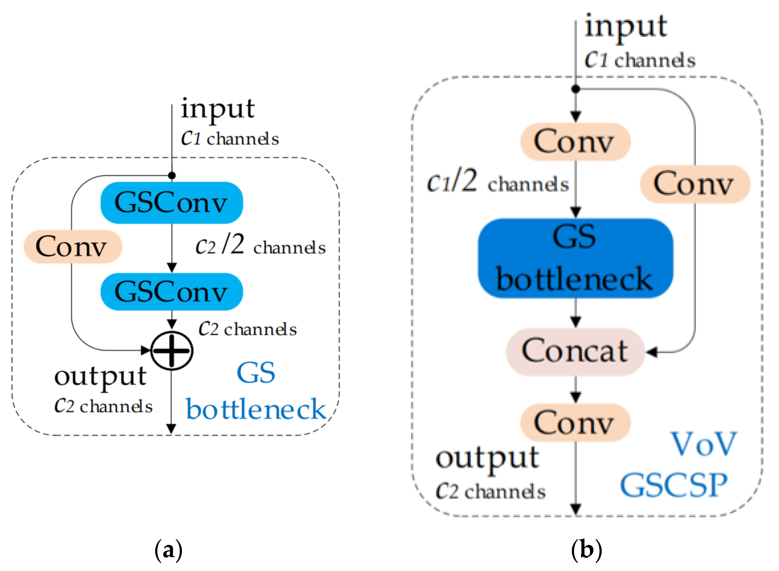
CNN have been shown to have better image detection accuracy compared to conventional image recognition methods. However, the deployment of agricultural mobile embedded devices is frequently constrained due to the high model complexity, significant computational cost, and memory-intensive nature of the devices. To address this issue, several light-weight networks such as Ghostnet [29], Mobilenet [30,31,32], and ShuffleNet [33] were developed, which effectively balance speed and accuracy. Among these networks, ShuffleNet V2 demonstrated higher accuracy than MobileNet V2 and Ghostnet for the same complexity. To reduce the number of parameters in the network, ShuffleNet V2 was selected as the backbone network for Yolov5 in this study.

In 2018, the authors of ShuffleNet V2 proposed four design principles for effective networks because they felt that the computational model complexity should not only take into account FLOPs but also factors such as memory access time cost (MAC) and degree of parallelism [34]. The structure of the ShuffleNet V2 network was divided into two units, as shown in Figure 4. The basic unit (1) split the feature image into two branches, the c-c’ channel and the c’ channel, one of which was left unchanged and the other of which had two 1 × 1 convolutions and one 3 × 3 convolution. The data from these two branches were then connected to concat, which equalized the number of input and output channels and complied with the G1 and G4 designs. The base unit (2) removed the operation of channel splitting to double the number of output channels, and the left and right branching operations were the same as in unit (a).

2.3.3. Slim-Neck

In CNNs, accelerating prediction computation is crucial. One technique to achieve this is the use of channel-sparse convolution (DSC), which severs hidden connections between each channel when transferring image space information. However, compressing the spatial dimensions (height and width) and expanding channels results in some loss of semantic information. On the other hand, channel-dense convolution (SC) maximizes information preservation between each channel. The authors combined SC and DSC through shuffle to create a new hybrid convolution called Ghost-Shuffle Convolution (GSConv) [35], as shown in Figure 5. This involved convolving the input feature map with C1 channels (C1 is the number of channels of the input feature map) to generate a C1/2 feature vector, obtaining another C1/2 feature vector through Depth Wise Convolution (DW Conv), concatenating the two feature vectors, and finally permuting the SC-generated information to each DSC part through channel shuffle. The number of channels of the output feature map was C2. The resulting nonlinear expression capability of GSConv was enhanced. The method achieved output similar to the standard convolution with a 50% reduction in computational cost. The time complexity of convolutional computation is defined by FLOPs. Therefore, without bias, the time complexity of SC, DSC, and GSConv can be expressed as follows:

$$\mathrm{T}\mathrm{i}\mathrm{m}{\mathrm{e}}_{\mathrm{S}\mathrm{C}}=\mathrm{W}\times \mathrm{H}\times {\mathrm{K}}_{\mathrm{w}}\times {\mathrm{K}}_{\mathrm{h}}\times \mathrm{C}1\times \mathrm{C}2$$

(4)

$$\mathrm{T}\mathrm{i}\mathrm{m}{\mathrm{e}}_{\mathrm{D}\mathrm{S}\mathrm{C}}=\mathrm{W}\times \mathrm{H}\times {\mathrm{K}}_{\mathrm{w}}\times {\mathrm{K}}_{\mathrm{h}}\times 1\times \mathrm{C}2$$

(5)

$$\mathrm{T}\mathrm{i}\mathrm{m}{\mathrm{e}}_{\mathrm{G}\mathrm{S}\mathrm{C}\mathrm{o}\mathrm{n}\mathrm{v}}=\mathrm{W}\times \mathrm{H}\times {\mathrm{K}}_{\mathrm{w}}\times {\mathrm{K}}_{\mathrm{h}}\times \frac{\mathrm{C}2}{2}\times (\mathrm{C}1+1)$$

(6)

where W is the width of the output feature map; H is the height of the output feature map; K_w, K_h is the size of the convolution kernel; C1 is the number of channels of the input feature map; C2 is the number of channels of the output feature map.

VOV-GSCSP (one-time aggregation cross stage partial network module) is the cross stage partial network (GSCSP) module designed by a one-time aggregation method. Its structure introduces a Ghost-Shuffle (GS) bottleneck that is designed on the basis of GSconv to reduce the complexity of the computation and network structure while maintaining sufficient accuracy. The structure of the GS bottleneck is shown in Figure 6a; the structure of VOV-GSCSP is shown in Figure 6b. In the VOV-GSCSP, the input feature image is divided into two branches after one convolution, one branch is kept unchanged, the other branch is subjected to GS bottleneck convolution operations, and the information from the two branches is connected to concat and output after one convolution operation. Finally, the slim-neck layer can be constructed by using the GSConv and VoV-GSCSP models flexibly.

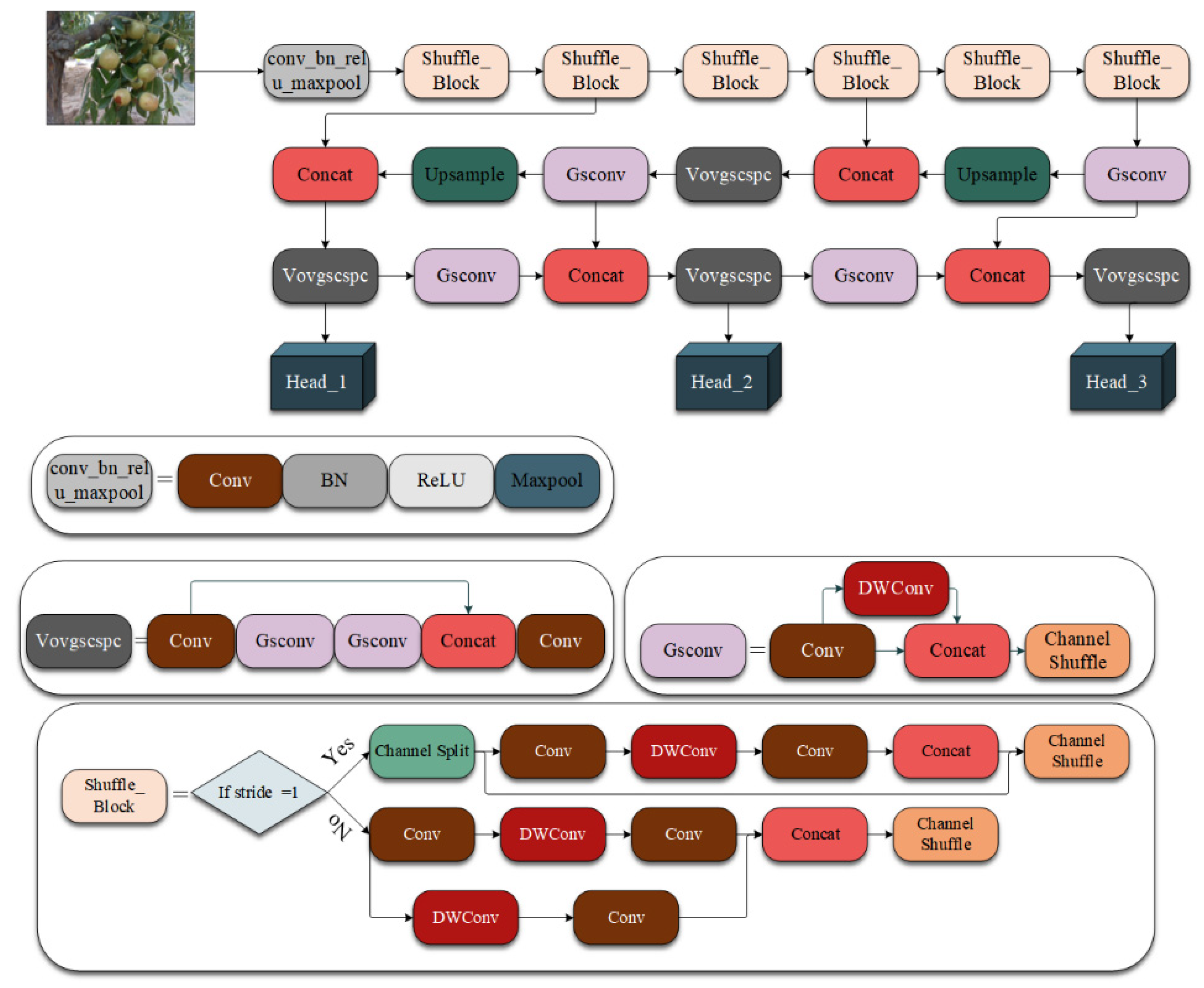
2.3.4. Optimized Method

Knowledge distillation was a common approach to obtaining an efficient, lightweight model. The idea was to use a large accurate trained network to train a lightweight network [36]. The large network, also known as the “teacher network”, was a more complex network model with very good performance and generalization capabilities; the lightweight network, also known as the “student network”, had fewer parametric operations and was more suitable for deployment in embedded devices. Using the knowledge distillation method, the simpler and less parametric student network can have similar performance to the teacher network [37]. The distillation process is shown in Figure 7.

Firstly, the teacher network and the student network were trained to obtain the logits of the two networks, respectively; the logits of the teacher network and the student network were distilled at a temperature of T, respectively. After the softmax layer to obtain the predicted probability distributions of the teacher network and student network categories (soft labels and soft prediction, respectively), the loss function ${\mathrm{L}}_{\mathrm{s}\mathrm{o}\mathrm{f}\mathrm{t}}$ can be further obtained. In the teacher network, there was also a certain error rate, and using the true label as the hard label can effectively reduce the probability that the teacher network spreads the error information to the student network, and the loss function ${\mathrm{L}}_{\mathrm{h}\mathrm{a}\mathrm{r}\mathrm{d}}$ can be obtained by calculation. The ${\mathrm{L}}_{\mathrm{s}\mathrm{o}\mathrm{f}\mathrm{t}}$ and ${\mathrm{L}}_{\mathrm{h}\mathrm{a}\mathrm{r}\mathrm{d}}$ were weighted to obtain the final distillation loss function ${\mathrm{L}}_{\mathrm{d}\mathrm{i}\mathrm{s}\mathrm{t}\mathrm{i}\mathrm{l}\mathrm{l}\mathrm{a}\mathrm{t}\mathrm{i}\mathrm{o}\mathrm{n}}$. The ${\mathrm{L}}_{\mathrm{s}\mathrm{o}\mathrm{f}\mathrm{t}}$, ${\mathrm{L}}_{\mathrm{h}\mathrm{a}\mathrm{r}\mathrm{d}}$, ${\mathrm{L}}_{\mathrm{d}\mathrm{i}\mathrm{s}\mathrm{t}\mathrm{i}\mathrm{l}\mathrm{l}\mathrm{a}\mathrm{t}\mathrm{i}\mathrm{o}\mathrm{n}}$ formulas are as follows:

$${\mathrm{L}}_{\mathrm{s}\mathrm{o}\mathrm{f}\mathrm{t}}=-{\displaystyle \sum _{\mathrm{j}}^{\mathrm{N}}{\mathrm{p}}_{\mathrm{j}}^{\mathrm{T}}\log ({\mathrm{q}}_{\mathrm{j}}^{\mathrm{T}})}$$

(7)

$${\mathrm{L}}_{\mathrm{h}\mathrm{a}\mathrm{r}\mathrm{d}}=-{\displaystyle \sum _{\mathrm{j}}^{\mathrm{N}}{\mathrm{c}}_{\mathrm{j}}\log ({\mathrm{q}}_{\mathrm{j}}^{\mathrm{T}})}$$

(8)

$${\mathrm{L}}_{\mathrm{d}\mathrm{i}\mathrm{s}\mathrm{t}\mathrm{i}\mathrm{l}\mathrm{l}\mathrm{a}\mathrm{t}\mathrm{i}\mathrm{o}\mathrm{n}}=(1-\alpha ){\mathrm{L}}_{\mathrm{s}\mathrm{o}\mathrm{f}\mathrm{t}}+\alpha {\mathrm{L}}_{\mathrm{h}\mathrm{a}\mathrm{r}\mathrm{d}}$$

(9)

where N is the total number of labels, ${\mathrm{p}}_{\mathrm{j}}^{\mathrm{T}}$ is the probability of the class j output from the softmax of the teacher network at temperature T, ${\mathrm{q}}_{\mathrm{j}}^{\mathrm{T}}$ is the probability of the class j output from the softmax of the student network at temperature T, ${\mathrm{c}}_{\mathrm{j}}$ is the true label value of class j, and α is the weighting coefficients.

2.4. Test Platform

The improved series of algorithms in this research were built in the Pytorch framework, and the software training environment configuration for the comparison experiments is shown in

Table 1. Experimental environment.

Configuration	Parameter
CPU	AMD EPYC 7642 48-CoreProcessor
GPU	NVIDIA GeForce RTX 3090
Accelerated environment	CUDA11.3
Deep learning framework	Pytorch 1.10
Programming language	Python 3.8

Where CPU is the Central Processing Unit; GPU is the Graphics Processing Unit.

.

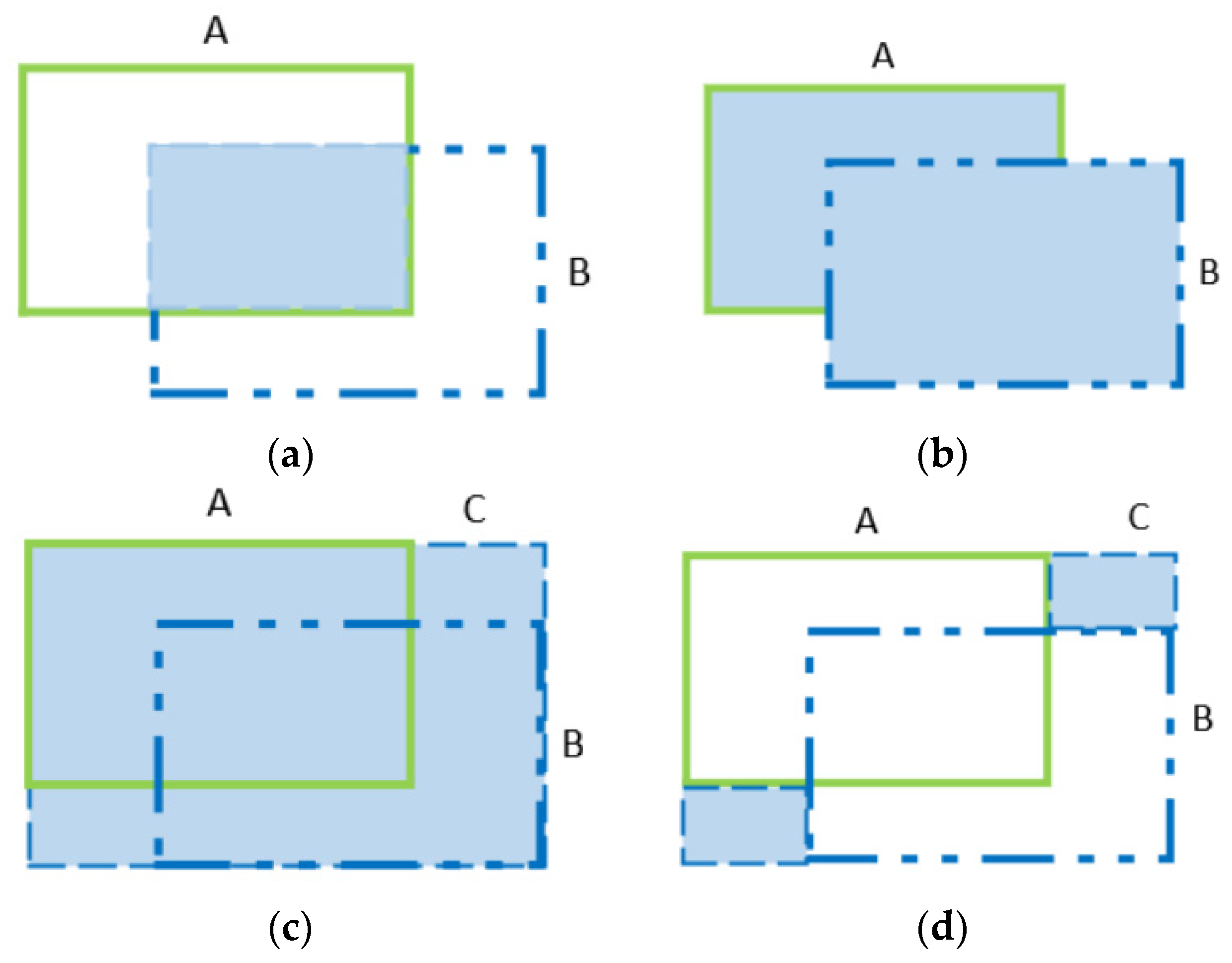
2.5. Evaluation of Model Performance

In this study, Precision, Recall, mean average Precision (mAP), F₁ score, Parameters, Model Size, and Frame per second (Fps) were used as model evaluation metrics, where Precision, Recall, mAP, F₁ score, and Parameters were formulated as follows:

$$\mathrm{P}\mathrm{r}\mathrm{e}\mathrm{c}\mathrm{i}\mathrm{s}\mathrm{i}\mathrm{o}\mathrm{n}=\frac{\mathrm{T}\mathrm{P}}{\mathrm{T}\mathrm{P}+\mathrm{F}\mathrm{P}}\times 100\%$$

(10)

$$\mathrm{R}\mathrm{e}\mathrm{c}\mathrm{a}\mathrm{l}\mathrm{l}=\frac{\mathrm{T}\mathrm{P}}{\mathrm{T}\mathrm{P}+\mathrm{F}\mathrm{N}}\times 100\%$$

(11)

$$\mathrm{m}\mathrm{A}\mathrm{P}=\frac{1}{\mathrm{C}}{\displaystyle \sum _{\mathrm{k}=\mathrm{i}}^{\mathrm{N}}\mathrm{P}(\mathrm{k})△}\mathrm{R}(\mathrm{k})\times 100\%$$

(12)

$${\mathrm{F}}_1=\frac{2\times \mathrm{P}\mathrm{r}\mathrm{e}\mathrm{c}\mathrm{i}\mathrm{s}\mathrm{i}\mathrm{o}\mathrm{n}\times \mathrm{R}\mathrm{e}\mathrm{c}\mathrm{a}\mathrm{l}\mathrm{l}}{\mathrm{P}\mathrm{r}\mathrm{e}\mathrm{c}\mathrm{i}\mathrm{s}\mathrm{i}\mathrm{o}\mathrm{n}+\mathrm{R}\mathrm{e}\mathrm{c}\mathrm{a}\mathrm{l}\mathrm{l}}\times 100\%$$

(13)

$$\mathrm{P}\mathrm{a}\mathrm{r}\mathrm{a}\mathrm{m}\mathrm{e}\mathrm{t}\mathrm{e}\mathrm{r}\mathrm{s}={\mathrm{C}}_{\mathrm{o}}\times ({\mathrm{C}}_{\mathrm{i}}\times {\mathrm{K}}_{\mathrm{w}}\times {\mathrm{K}}_{\mathrm{h}}+1)$$

(14)

where TP, FP, and FN represent the number of true positive samples, false positive samples, and false negative samples, respectively. C is the number of classes, N is the number of referenced thresholds, k is the threshold, P(k) is the precision rate, R(k) is the Recall rate, C_o represents the number of input channels, and C_i is the size of the convolution kernel. Recall and Precision are two of the important indexes for evaluating the model. The larger the area of the Precision–Recall curve, the better the comprehensive performance of the model. mAP is a measure of detection accuracy in target detection, and the higher the mAP, the better the detection effect of the model. The F₁ score is the weighted average of model Precision and Recall, and the larger the F₁ value, the more stable the model is. Fps is the number of images per second that the image is transmitted. Fps is an evaluation index of detection speed; the transmission of images is more fluid as Fps increases.

3. Results

3.1. Improved Yolov5s Model Based on Ablation Experiment

In order to construct a winter jujube detection model, this study tested using different structural models on a winter jujube dataset in a natural environment, and the effectiveness of different structures was verified. To ensure the reliability of the experiments, this study was conducted under the same training and validation sets with an epoch of 300 and batch size of 16. The results are shown in

Table 2. Comparative experimental results of improvement process.

Model	Precision (%)	Recall (%)	mAP (%)	F1 Score (%)	Parameters	Model Size (MB)	Fps
Yolov5s	84.00	80.70	88.90	82.31	7,012,822	13.74	106.38
Yolov5s + Shufflenetv2	83.40	81.40	87.90	82.38	842,358	2.06	114.94
Yolov5s + GSconv	87.70	81.80	89.50	84.64	6,581,366	13.58	111.11
Yolov5s + VoVGSCSPC	88.10	82.40	89.90	85.15	7,189,030	14.83	107.52
Yolov5s + Shufflenetv2 + GSconv	84.90	80.90	88.60	82.85	736,630	1.85	105.26
Yolov5s + Shufflenetv2 + VoVGSCSPC	85.10	80.60	88.70	82.78	889,422	2.19	111.11
Yolov5s + Slim-neck	88.20	82.30	89.40	85.14	6,737,702	13.96	107.52
Yolov5s + Shufflenetv2 + Slim-neck	86.30	81.10	89.40	83.61	787,230	1.91	109.89

.

From Table 2, it can be seen that the parameter number of Yolov5s was 7,012,822, and the Model size is 13.74 MB. After replacing the backbone network with Shufflenet V2, the Parameters and Model size are significantly reduced, but at the same time, the Precision and mAP are also slightly reduced. In order to meet the light weight and at the same time ensure the accuracy of the model target recognition, the model neck layer is replaced with a slim-neck. The improved Yolov5s model parameter number is 787,230, which is 88.77% less than Yolov5s; the Model size is 1.91MB, which is 86.09% smaller. Precision, Recall, mAP, and F₁ scores are elevated by 2.30%, 0.40%, 0.50%, and 1.30%, respectively.

3.2. Improved Yolov5s Model

Yolo, as an efficient single-target detection framework, has excellent recognition accuracy and speed. Among them, Yolov5s, as the model with the smallest depth and feature map width in the Yolov5 series, is often deployed in agricultural mobile embedded devices. In order to better cope with the complexity of the agricultural production environment, in this research we replaced the backbone network of Yolov5s with the ShuffleNet V2 to reduce the number of parameters in the network. The slim-neck model was built using GSConv and VoV-GSCSP and replaced the original neck structure of Yolov5s to reduce the complexity of the model and improve the detection accuracy at the same time. The improved Yolov5s model framework is shown in Figure 8.

3.3. Performance Comparison with Other Lightweight Backbone Networks

To meet the deployment requirements of the model in embedded devices, this study improved the backbone network of the model using Shufflenet V2, which greatly reduced the model size and complexity of the model. Current mainstream lightweight backbone networks include Ghostnet, Mobilenet, etc. Ghostnet was proposed by Huawei’s Noah’s Ark Lab in 2020, which aimed to obtain more feature graph information with less computation. MobileNet was first proposed by Google in 2017, which was an efficient model for mobile and embedded devices. Mobilenetv3 had some improvements based on Mobilenetv1 and Mobilenetv2, and the network performance has been improved compared to previous generations. In order to further verify the effectiveness of the improved Yolov5s model, in this study, Ghostnet and mobilenetv3 were used to replace the backbone network of the improved model for the target detection of winter jujube under the same dataset and compared with the improved model, and the comparison data of the three different lightweight models are shown in

Table 3. The model performance with different lightweight models.

Model	Precision (%)	Recall (%)	mAP (%)	F1 Score (%)	Parameters	Model Size (MB)	Fps
Yolov5s	84.00	80.70	88.90	82.31	7,012,822	13.74	106.38
Yolov5s + Ghostnet + Slim-neck	86.60	83.50	91.00	85.02	4,803,854	10.10	98.49
Yolov5s + Mobilenetv3 + Slim-neck	86.50	80.20	88.60	83.23	1,327,268	3.10	87.51
Yolov5s + Shufflenet V2 + Slim-neck	86.30	81.10	89.40	83.61	787,230	1.91	109.89

. The results showed that the model with the addition of Ghostnet has a better detection effect, but its Parameters and Model size are significantly increased compared with the improved Yolov5s model of this study; they were 6.1 times and 5.3 times the improved Yolov5s model of this study, respectively. On the other hand, the incorporated mobilenetv3 model has the lowest Fps, which is 79.63% of the improved Yolov5s model. Shufflenet V2, which acts as the backbone network, can balance model accuracy, size, and speed and is more suitable for deployment in agricultural mobile embedded devices.

3.4. Further Optimized Yolov5s Model Based on Knowledge Distillation

Due to various factors such as the distance of the camera from the fruit, the overlapping of fruits, and obstruction from tree branches and leaves in the natural environment, the improved yolov5s model before distillation could not extract enough information about the fruit features, which resulted in the model missing the detection of small target fruits and fruits in areas with large obstructions, as illustrated in Figure 9b,f.

In terms of knowledge distillation as a mainstream knowledge transfer method, the improved Yolov5s network (student network) was trained with the Yolov5m network (teacher network), which has higher model complexity to enhance the generalization ability of the student network and improve the model accuracy without increasing the number of parameters. As shown in Figure 9c,g, the distilled model has better recognition of the obscured fruits and small target fruits. The comparison data before and after distillation are shown in

Table 4. The model performance with different models.

Model	Precision (%)	Recall (%)	mAP (%)	F1 Score (%)	Parameters	Model Size (MB)	Fps
Yolov5m model	91.40	83.70	91.20	87.38	20,852,934	42.24	50.76
Improved Yolov5s model	86.30	81.10	89.40	83.61	787,230	1.91	109.89
Optimized Yolov5s model	88.70	82.00	90.80	85.21	787,230	1.91	109.89

. Compared with before distillation, the Precision, Recall, mAP, and F₁ scores of the student network have significantly improved, increasing about 2.40%, 0.90%, 1.40%, and 1.60%, respectively, and the number of parameters and model size have not changed compared with those before distillation. Thus, it can be seen that the final optimized Yolov5s model was obtained to ensure high accuracy and performance while significantly reducing the number of parameters, computational volume, and model size.

The loss curve reflects the dynamic variation of the network training, and we can see whether the trained model converges, fits, or contains other information. Usually, the smaller the loss function, the better the robustness of the model. The loss function of the model before and after distillation is shown in Figure 10. The results show that the value of the loss function of the model after distillation converges around 0.096, and the value of the loss function of the model before distillation converges around 0.110. The value of the loss function of the model after distillation is lower than that before distillation, which proves that the performance of the model can be further enhanced after knowledge distillation.

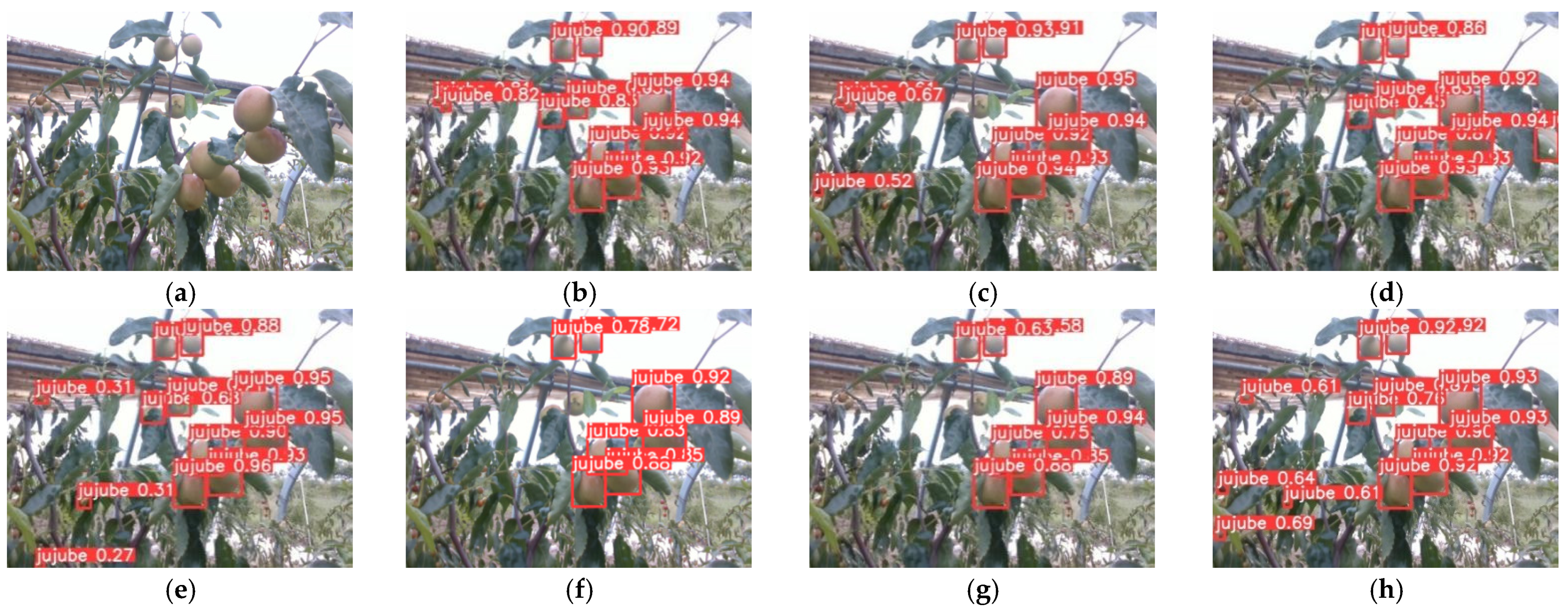
3.5. Performance Comparison of Target Detection Using Different Algorithms

To further verify the effectiveness of the optimized Yolov5s model, the Yolov3-tiny, Yolov4-tiny, Yolov7-tiny [38], SSD [39], and Faster RCNN models were selected for comparison with the optimized Yolov5s model in this study. To ensure the reliability of the experiments, this study was conducted under the same training and validation sets with an epoch of 300 and batch size of 16. The validation results for each model are shown in Figure 11. The comparative data for each model are shown in

Table 5. The model performance with different model.

Model	Precision (%)	Recall (%)	mAP (%)	F1 Score (%)	Parameters	Model Size (MB)	Fps
Yolov5s	84.00	80.70	88.90	82.31	7,012,822	13.74	106.38
Yolov3-tiny	84.52	79.21	87.59	81.77	8,666,692	17.44	163.96
Yolov4-tiny	83.38	80.24	85.76	81.77	6,056,606	23.57	151.46
Yolov7-tiny	87.90	81.60	88.50	84.63	6,007,596	12.29	109.69
SSD	91.60	52.10	77.91	66.42	26,285,486	90.60	57.03
Faster RCNN	52.27	72.05	67.68	60.58	137,098,724	108.17	8.07
Optimized Yolov5s model	88.70	82.00	90.80	85.21	787,230	1.91	109.89

.

The P–R curve is a curve with Recall as the horizontal coordinate and Precision as the vertical coordinate, and its area can be expressed as the comprehensive performance of the winter jujube target detection model. As can be seen from Figure 12, the curve area of the Yolo series is significantly larger than that of the SSD and Faster RCNN, which indicates that the Yolo series models have a fine detection effect for winter jujube target detection.

4. Discussion

As shown in Figure 10, we can see that YOLOv3-tiny, YOLOv4-tiny, SSD, and Faster rcnn miss more small target fruits and leaf-obscured fruits, among which SSD and Faster RCNN miss the most fruits. For Faster RCNN, the convolutional extraction network, regardless of whether VGGNet or ResNet was used, the extracted feature maps were single-layer and the resolution was smaller. Therefore, there is a problem of inadequate feature extraction for those images with multiple scales and small targets. Although SSD uses the idea of a pyramidal feature layer, it uses the conv4_3 large scale feature map to detect small targets, and the number of convolution layers in the largescale feature map is small. A 32 × 32 target only gets 4 × 4 images after convolution, and the acquired feature information is not sufficient.

As shown in Table 5. Yolov5s, as an improved detection network over Yolov3-tiny and Yolov4-tiny, has the smallest model size and the highest F₁ score compared with Yolov3-tiny and Yolov4-tiny; although its Fps is smaller than that of Yolov3-tiny and Yolov4-tiny, it also reaches 106.38, which meets the demand for real-time detection. Compared with Yolov5s, the Precision, Recall, mAP, and F₁ score of the optimized Yolov5s model in this study are improved by 4.70%, 1.30%, 1.90%, and 2.90%, respectively. Meanwhile, the model Parameters and Model size decrease substantially, by 88.77% and 86.09%, respectively. In addition, the F₁ value of the optimized Yolov5s model is the highest among all models, reaching 85.21%. Yolov7 is the latest generation of target detection algorithm in the Yolo series, and Yolov7-tiny, as a lightweight network of Yolov7, has lower Precision, Recall, mAP, and F₁ value than the optimized Yolov5s model in this study, and the model size is 6.43 times larger than the optimized Yolov5s model.

In order to simulate the processor of an embedded device, the Intel (R) Core (TM) i7-10875H CPU was chosen for this study for winter jujube object detection. The test results of the optimized model in this study for different scenes are shown in Figure 13, and the Fps reached 29.41, satisfying the demand for the real-time detection of embedded devices. From Figure 13a, c–f it can be seen that the optimized model has good detection results in the environments of bright light, single targets, multiple targets, behind branch and leaves, and broken Fruit. However, in dim light scenes, the optimized model does not detect well, as shown in Figure 13b.

In order to evaluate the optimized model’s performance in dim light conditions, this study selected images from the test set that were captured in dim light for re-detection. The resulting Precision and Recall of the test results were 86.10% and 80.60%, respectively. The missed fruit were mainly due to large, shaded areas and large areas of obscured fruit, as shown in Figure 14e,f. These results may be attributed to the overall dark color of the image caused by the dim light, which makes it difficult to distinguish between the winter jujube and the background. In addition, the model extracted fewer features of the jujube fruit in this dim light environment, resulting in a slightly less effective identification of the fruit.

In conclusion, the optimized yolov5s model outperforms current mainstream target detection networks in winter jujube target detection. Future work should focus on improving the model’s feature extraction capability by adding light compensation and enriching the dataset of winter jujube under dim light conditions. In addition, we should consider adding different types of winter jujube at different stages of maturity in order to “pick ripe and leave green” during the picking process.

5. Conclusions

In this study, an optimized lightweight Yolov5s-based target detection algorithm for winter jujube was established to achieve the accurate recognition of jujube fruits while reducing the model’s size. Shufflenet V2 was chosen instead of Yolov5’s backbone network in this study, which can effectively reduce the model parameters and size. In winter jujube target detection, Shufflenet V2 has better performance compared with other lightweight backbone networks. In addition, this study also used GSConv and VoV-GSCSP to build a slim-neck to replace Yolov5’s original neck structure in order to achieve accuracy of winter jujube detection while reducing the complexity of the model. Finally, this study selects knowledge distillation as a method of model optimization to enhance the generalization ability of the network and improve model accuracy without increasing the Parameters. The optimized Yolov5s model improves the recognition of obscured fruits and small target fruits and maintains high accuracy, and has good performance in the target detection of winter jujube and is applicable to the practical application of small target detection, such as other jujube species.

References

1. Feng, J.; Liu, G.; Si, Y.; Wang, S.; Zhou, W. Construction of a laser vision system for an apple picking robot. Trans. Chin. Soc. Agric. Eng. 2013, 29, 32–37. [Google Scholar]
2. Xie, E.; Ding, J.; Wang, W.; Zhan, X.; Xu, H.; Sun, P.; Li, Z.; Luo, P. Detco: Unsupervised contrastive learning for object detection. In Proceedings of the IEEE/CVF International Conference on Computer Vision, Montreal, BC, Canada, 11–17 October 2021; pp. 8392–8401. [Google Scholar]
3. Zhao, M.; Jha, A.; Liu, Q.; Millis, B.A.; Mahadevan-Jansen, A.; Lu, L.; Landman, B.A.; Tyska, M.J.; Huo, Y. Faster Mean-shift: GPU-accelerated clustering for cosine embedding-based cell segmentation and tracking. Med. Image Anal. 2021, 71, 102048. [Google Scholar] [CrossRef] [PubMed]
4. Zhao, M.; Liu, Q.; Jha, A.; Deng, R.; Yao, T.; Mahadevan-Jansen, A.; Tyska, M.J.; Millis, B.A.; Huo, Y. VoxelEmbed: 3D Instance Segmentation and Tracking with Voxel Embedding Based Deep Learning; Springer International Publishing: Cham, Switzerland, 2021; pp. 437–446. [Google Scholar]
5. You, L.; Jiang, H.; Hu, J.; Chang, C.H.; Chen, L.; Cui, X.; Zhao, M. GPU-accelerated Faster Mean Shift with euclidean distance metrics. In Proceedings of the 2022 IEEE 46th Annual Computers, Software, and Applications Conference, Los Alamitos, CA, USA, 27 June–1 July 2022; pp. 211–216. [Google Scholar]
6. Zheng, Z.; Hu, Y.; Yang, H.; Qiao, Y.; He, Y.; Zhang, Y.; Huang, Y. AFFU-Net: Attention feature fusion U-Net with hybrid loss for winter jujube crack detection. Comput. Electron. Agric. 2022, 198, 107049. [Google Scholar] [CrossRef]
7. Zheng, Z.; Yang, H.; Zhou, L.; Yu, B.; Zhang, Y. HLU 2-Net: A residual U-structure embedded U-Net with hybrid loss for tire defect inspection. IEEE Trans. Instrum. Meas. 2021, 70, 1–11. [Google Scholar]
8. Yang, Q.; Duan, S.; Wang, L. Efficient Identification of Apple Leaf Diseases in the Wild Using Convolutional Neural Networks. Agronomy 2022, 12, 2784. [Google Scholar] [CrossRef]
9. Fu, L.; Yang, Z.; Wu, F.; Zou, X.; Lin, J.; Cao, Y.; Duan, J. YOLO-Banana: A lightweight neural network for rapid detection of banana bunches and stalks in the natural environment. Agronomy 2022, 12, 391. [Google Scholar] [CrossRef]
10. Moreira, G.; Magalhães, S.A.; Pinho, T.; dos Santos, F.N.; Cunha, M. Benchmark of deep learning and a proposed hsv colour space models for the detection and classification of greenhouse tomato. Agronomy 2022, 12, 356. [Google Scholar] [CrossRef]
11. Krizhevsky, A.; Sutskever, I.; Hinton, G.E. Imagenet classification with deep convolutional neural networks. Commun. ACM 2017, 60, 84–90. [Google Scholar] [CrossRef] [Green Version]
12. Simonyan, K.; Zisserman, A. Very deep convolutional networks for large-scale image recognition. arXiv 2014, arXiv:1409.1556. [Google Scholar]
13. Szegedy, C.; Liu, W.; Jia, Y.; Sermanet, P.; Reed, S.; Anguelov, D.; Erhan, D.; Vanhoucke, V.; Rabinovich, A. Going deeper with convolutions. In Proceedings of the IEEE Conference on Computer Vision and Pattern Recognition, Boston, MA, USA, 7–12 June 2015; pp. 1–9. [Google Scholar]
14. Long, J.; Shelhamer, E.; Darrell, T. Fully convolutional networks for semantic segmentation. In Proceedings of the IEEE Conference on Computer Vision and Pattern Recognition, Boston, MA, USA, 7–12 June 2015; pp. 3431–3440. [Google Scholar]
15. Williams, H.A.; Jones, M.H.; Nejati, M.; Seabright, M.J.; Bell, J.; Penhall, N.D.; Barnett, J.J.; Duke, M.D.; Scarfe, A.J.; Ahn, H.S.; et al. Robotic kiwifruit harvesting using machine vision, convolutional neural networks, and robotic arms. Biosyst. Eng. 2019, 181, 140–156. [Google Scholar] [CrossRef]
16. Girshick, R.; Donahue, J.; Darrell, T.; Malik, J. Rich feature hierarchies for accurate object detection and semantic segmentation. In Proceedings of the IEEE Conference on Computer Vision and Pattern Recognition, Columbus, OH, USA, 23–28 June 2014; pp. 580–587. [Google Scholar]
17. Girshick, R. Fast r-cnn. In Proceedings of the IEEE International Conference on Computer Vision, Santiago, Chile, 7–13 December 2015; pp. 1440–1448. [Google Scholar]
18. Ren, S.; He, K.; Girshick, R.; Sun, J. Faster r-cnn: Towards real-time object detection with region proposal networks. Adv. Neural Inf. Process. Syst. 2017, 39, 1137–1149. [Google Scholar] [CrossRef] [PubMed] [Green Version]
19. Redmon, J.; Divvala, S.; Girshick, R.; Farhadi, A. You only look once: Unified, real-time object detection. In Proceedings of the IEEE Conference on Computer Vision and Pattern Recognition, Las Vegas, NV, USA, 27–30 June 2016; pp. 779–788. [Google Scholar]
20. Redmon, J.; Farhadi, A. Yolov3: An incremental improvement. arXiv 2018, arXiv:1804.02767. [Google Scholar]
21. Bochkovskiy, A.; Wang, C.Y.; Liao, H.Y.M. Yolov4: Optimal speed and accuracy of object detection. arXiv 2020, arXiv:2004.10934. [Google Scholar]
22. Yan, B.; Fan, P.; Lei, X.; Liu, Z.; Yang, F. A real-time apple targets detection method for picking robot based on improved YOLOv5. Remote Sens. 2021, 13, 1619. [Google Scholar] [CrossRef]
23. Hu, J.; Shen, L.; Sun, G. Squeeze-and-excitation networks. In Proceedings of the IEEE Conference on Computer Vision and Pattern Recognition, Salt Lake City, UT, USA, 18–23 June 2018; pp. 7132–7141. [Google Scholar]
24. Zhou, J.; Hu, W.; Zou, A.; Zhai, S.; Liu, T.; Yang, W.; Jiang, P. Lightweight detection algorithm of kiwifruit based on improved YOLOX-s. Agriculture 2022, 12, 993. [Google Scholar] [CrossRef]
25. Sozzi, M.; Cantalamessa, S.; Cogato, A.; Kayad, A.; Marinello, F. Automatic bunch detection in white grape varieties using YOLOv3, YOLOv4, and YOLOv5 deep learning algorithms. Agronomy 2022, 12, 319. [Google Scholar] [CrossRef]
26. Qiao, Y.; Hu, Y.; Zheng, Z.; Yang, H.; Zhang, K.; Hou, J.; Guo, J. A Counting Method of Red Jujube Based on Improved YOLOv5s. Agriculture 2022, 12, 2071. [Google Scholar] [CrossRef]
27. He, K.; Zhang, X.; Ren, S.; Sun, J. Spatial pyramid pooling in deep convolutional networks for visual recognition. IEEE Trans. Pattern Anal. Mach. Intell. 2015, 37, 1904–1916. [Google Scholar] [CrossRef] [Green Version]
28. Liu, S.; Qi, L.; Qin, H.; Shi, J.; Jia, J. Path aggregation network for instance segmentation. In Proceedings of the IEEE Conference on Computer Vision and Pattern Recognition, Salt Lake City, UT, USA, 18–23 June 2018; pp. 8759–8768. [Google Scholar]
29. Han, K.; Wang, Y.; Tian, Q.; Guo, J.; Xu, C.; Xu, C. Ghostnet: More features from cheap operations. In Proceedings of the IEEE/CVF Conference on Computer Vision and Pattern Recognition, New Orleans, LA, USA, 18–24 June 2022; pp. 1580–1589. [Google Scholar]
30. Howard, A.G.; Zhu, M.; Chen, B.; Kalenichenko, D.; Wang, W.; Weyand, T.; Andreetto, M.; Adam, H. Mobilenets: Efficient convolutional neural networks for mobile vision applications. arXiv 2017, arXiv:1704.04861. [Google Scholar]
31. Sandler, M.; Howard, A.; Zhu, M.; Zhmoginov, A.; Chen, L.C. Mobilenetv2: Inverted residuals and linear bottlenecks. In Proceedings of the IEEE Conference on Computer Vision and Pattern Recognition, Salt Lake City, UT, USA, 18–23 June 2018; pp. 4510–4520. [Google Scholar]
32. Howard, A.; Sandler, M.; Chu, G.; Chen, L.C.; Chen, B.; Tan, M.; Wang, W.; Zhu, Y.; Pang, R.; Vasudevan, V.; et al. Searching for mobilenetv3. In Proceedings of the IEEE/CVF International Conference on Computer Vision, Seoul, Republic of Korea, 27 October–2 November 2019; pp. 1314–1324. [Google Scholar]
33. Zhang, X.; Zhou, X.; Lin, M.; Sun, J. Shufflenet: An extremely efficient convolutional neural network for mobile devices. In Proceedings of the IEEE Conference on Computer Vision and Pattern Recognition, Salt Lake City, UT, USA, 18–23 June 2018; pp. 6848–6856. [Google Scholar]
34. Ma, N.; Zhang, X.; Zheng, H.T.; Sun, J. Shufflenet v2: Practical guidelines for efficient cnn architecture design. In Proceedings of the European Conference on Computer Vision (ECCV), Munich, Germany, 8–14 September 2018; pp. 116–131. [Google Scholar]
35. Li, H.; Li, J.; Wei, H.; Liu, Z.; Zhan, Z.; Ren, Q. Slim-neck by GSConv: A better design paradigm of detector architectures for autonomous vehicles. arXiv 2022, arXiv:2206.02424. [Google Scholar]
36. Mehta, R.; Ozturk, C. Object detection at 200 frames per second. In Proceedings of the European Conference on Computer Vision (ECCV) Workshops, Munich, Germany, 8–14 September 2018; Part V 15. pp. 659–675. [Google Scholar]
37. Chen, G.; Choi, W.; Yu, X.; Han, T.; Chandraker, M. Learning efficient object detection models with knowledge distillation. Adv. Neural Inf. Process. Syst. 2017, 30, 1–10. [Google Scholar]
38. Wang, C.Y.; Bochkovskiy, A.; Liao, H.Y.M. YOLOv7: Trainable bag-of-freebies sets new state-of-the-art for real-time object detectors. arXiv 2022, arXiv:2207.02696. [Google Scholar]
39. Liu, W.; Anguelov, D.; Erhan, D.; Szegedy, C.; Reed, S.; Fu, C.Y.; Berg, A.C. Ssd: Single shot multibox detector. In Proceedings of the European Conference on Computer Vision, Amsterdam, The Netherlands, 11–14 October 2016; pp. 21–37. [Google Scholar]
Figure 1. Winter jujubes in different scenes. (a) Bright light; (b) Dim light; (c) Single target; (d) Multiple targets; (e) Behind branch and leaves; (f) Broken Fruit.
Agronomy 13 00810 g001
Figure 2. Image sample after data expansion. (a) Original image; (b) Mirroring image; (c) Adding noise; (d) Rotation; (e) Rotation + Reduced brightness + erasure; (f) Adding noise + Rotation + erasure.
Agronomy 13 00810 g002
Figure 3. The details of GIOU. (a) A ∩ B; (b) A ∪ B; (c) C; (d) C − (A ∪ B).
Agronomy 13 00810 g003
Figure 4. The structure of ShuffleNet-V2 Units: (a) the structure of ShuffleNet-V2 Unit1; (b) the structure of ShuffleNet-V2 Unit2.
Agronomy 13 00810 g004
Figure 5. The structure of the GSConv. Where GSConv is the Ghost-Shuffle Convolution; DW Conv is the Depth Wise Convolution; C1 is the number of channels of the input feature map; C2 is the number of channels of the output feature map.
Agronomy 13 00810 g005
Figure 6. The structure of the GS bottleneck and VOV-GSCSP. (a) the structures of the GS bottleneck; (b) the structures of the VOV-GSCSP. Where GS bottleneck is the Ghost-Shuffle bottleneck; VOV-GSCSP is one-time aggregation cross stage partial network module.
Agronomy 13 00810 g006
Figure 7. Distillation process.
Agronomy 13 00810 g007
Figure 8. The structure of improved Yolov5s model. Where conv_bn_relu_maxpool is composed of Conv, Bn, ReLu and Maxpool; Bn is the Batch normalization; ReLu is the Rectified Linear Unit; Maxpool is the operation to calculate the maximum value of all elements in the pooling window.
Agronomy 13 00810 g008
Figure 9. Original image and the results of different models for the recognition of jujube: (a) the original image of large area obscuring jujube; (b) the improved Yolov5s model to large area obscuring jujube detection image; (c) the optimized Yolov5s model to large area obscuring jujube detection image; (d) the Yolov5m to large area obscuring jujube detection image; (e) the original image of small target jujube; (f) the improved Yolov5s model to small target jujube detection image; (g) the optimized Yolov5s model to small target jujube detection image; (h) the Yolov5m to small target jujube detection image. Where the yellow boxes are the label boxes marked manually of unidentified winter jujube, and the red boxes are the test results of model test.
Agronomy 13 00810 g009
Figure 10. Comparison of loss before and after model distillation: (a) Student Net before knowledge distillation; (b) Student Net after knowledge distillation.
Agronomy 13 00810 g010
Figure 11. Original image and test results of different algorithms. (a) Original image; (b) Yolov5s; (c) Yolov3-tiny; (d) Yolov4-tiny; (e) Yolov7-tiny; (f) SSD; (g) Faster RCNN; (h) Optimized Yolov5s model.
Agronomy 13 00810 g011
Figure 12. The PR curve of winter jujubes with different target detection algorithms.
Agronomy 13 00810 g012
Figure 13. Test results of different scenes. (a) Bright light; (b) Dim light; (c) Single target; (d) Multiple targets; (e) Shading by branch and leaves; (f) Broken Fruit.
Agronomy 13 00810 g013
Figure 14. Original image and test results of different scenes in dim light conditions. (a) Scene 1; (b) Scene 2; (c) Scene 3; (d) test results of scene 1; (e) test results of scene 2; (f) test results of scene 3. The yellow boxes are the label boxes marked manually of unidentified winter jujube.
Agronomy 13 00810 g014