Article

Machine Learning Models of Exergoenvironmental Damages and Emissions Social Cost for Mushroom Production

by
Ashkan Nabavi-Pelesaraei
1,*,
Hassan Ghasemi-Mobtaker
2,*,
Marzie Salehi
2,
Shahin Rafiee
2,
Kwok-Wing Chau
3 and
Rahim Ebrahimi
4
1
Department of Mechanical Engineering of Biosystems, Faculty of Agriculture, Razi University, Kermanshah 6714414971, Iran
2
Department of Agricultural Machinery Engineering, Faculty of Agriculture, University of Tehran, Karaj 141556619, Iran
3
Department of Civil and Environmental Engineering, Hong Kong Polytechnic University, Kowloon ZS972, Hong Kong
4
Department of Mechanical Engineering of Biosystems, Faculty of Agriculture, Shahrekord University, Shahrekord 8815713471, Iran
*
Authors to whom correspondence should be addressed.
Agronomy 2023, 13(3), 737; https://doi.org/10.3390/agronomy13030737
Submission received: 19 January 2023 / Revised: 12 February 2023 / Accepted: 23 February 2023 / Published: 1 March 2023
(This article belongs to the Section Agricultural Biosystem and Biological Engineering)

Abstract

:
Applying conventional methods for prediction of environmental impacts in agricultural production is not actually applicable because they usually ignore other aspects such as useful energy and economic consequence. As such, this article evaluates intelligent models for exergoenvironmental damage and emissions social cost (ESC) for mushroom production in Isfahan province, Iran, by three machine learning (ML) methods, namely adaptive neuro-fuzzy inference system (ANFIS), artificial neural network (ANN), and support vector regression (SVR). Accordingly, environmental life cycle damages, cumulative exergy demand, and ESC are examined by the ReCiPe2016 method for 100 tons of mushroom production after data collection by interview. Exergoenvironmental results reveal that, in human health and ecosystems, direct emissions, and resources and exergy categories, diesel fuel and compost are the main hotspots. Economic analysis also shows that total ESC is about 1035$. Results of ML models indicate that ANN with a 6-8-3 structure is the optimum topology for forecasting outputs. Moreover, a two-level structure of ANFIS has weak results for prediction in comparison with ANN. However, support vector regression (SVR) with an absolute average relative error (AARE) (%) between 0.85 and 1.03 (based on specific unit), a coefficient of determination (R2) between 0.989 and 0.993 (based on specific unit), and a root mean square error (RMSE) between 0.003 and 0.011 (based on specific unit) is selected as the best ML model. It is concluded that ML models can furnish comprehensive and applicable exergoenvironmental-economical assessment of agricultural products.

1. Introduction

Button mushroom (Agaricus bisporus) is the most abundant cultivated mushroom, which is well known for its considerable economic benefits and plentiful medicinal and nutritional properties [1]. According to the FAO annual report in 2016, about 11 million tons (t) of mushrooms were produced in the world; Asian countries accounted for a significant share of this production [2]. Button mushroom production in Iran increased from 6997 to 152,378 t from 2001 to 2017, and approximately 10% of this was produced in Isfahan province [3].
Global warming, which is defined as consecutive increases in the earth’s atmospheric mean temperature, is one of the momentous topics in recent decades. It results from increased GHG concentration in the atmosphere, caused by human activities such as fossil fuels burning and deforestation [4]. GHG emissions from the agriculture sector are a direct result of food supply chains. Optimum and efficient use of energy and sources is the main condition for sustainable agriculture [5]. Life cycle assessment (LCA) is a known and powerful tool to assess environmental sustainability of technologies and products [6] and provide a systematic way to evaluate the advancements in source productivity [7]. Input production, storage, and distribution as well as usage with engine-based equipment lead to combustion of fossil fuels and the release of GHGs such as CO2, N2O and CH4 into the atmosphere and result in global warming [8].
Cumulative exergy demand (CExD) index is defined as the total exergy sum of all inputs needed to produce a crop [9]. In other words, the aim of CExD analysis is to make an efficient system or process to reduce loss or deterioration of exergy [10]. ESC is a fundamental tool, presenting useful information to help assess policies. ESC is defined as the marginal impact costs caused by emitting one extra t of greenhouse gas (CO2 eq) at any point in time, including ‘non-market’ impacts on human and environmental health [11]. The computation of carbon social cost, which is defined as the marginal damage cost of climate change, is a key strategy for the evaluation of climate policy [12].
For sustainable agricultural development, energy use, environmental effects, and cost efficiency are three important aspects at the center of attention [13]. The relationship between energy use and GHG emissions is intimate; therefore, there is a need to manage energy use in agriculture sector to decrease environmental footprints associated with input utilization. The energy consumption pattern varies according to management and agricultural systems, climate, and other conditions. Determining the relationship between environmental impacts and energy use is one of the most important steps in sustainable agriculture.
In recent years, linear methods have been used to model various agricultural and sometimes environmental phenomena. Their main disadvantage is that some real-world phenomena simply do not conform to the linear model assumptions. Hence, the need to use modern technologies, such as artificial intelligence and ML, increases significantly [14]. ML, within artificial intelligence, has been introduced as a useful tool to develop intelligent predictive algorithms in different applications. ML approaches have the ability to handle multivariate and multi-dimensional data and to discover hidden relationships within data in dynamic and complex conditions [15]. The applicability of various ML methods is generally quite different in various fields, problems, and types of data sets [16]. With respect to the mentioned methods, ANN is one of basic models of ML that includes competent soft computing techniques with effort simulating the human biological nervous system via linking different artificial elements, termed neurons [17].
Another intelligent system for modeling and forecasting is ANFIS [18]. It is a suitable method for the interpretation of non-linear systems [18]. Because ANFIS is the combination of fuzzy and ANN systems, it has the benefits of both models. In engineering issues where classical methods are too complicated to be used, this technique can be useful [19]. As the next model, SVM, based on Vapnik’s statistical learning theory, is widely used in some practical problems. Its main idea is to detect a separating hyperplane in between two parallel hyperplanes, where these two parallel hyperplanes are built according to the maximum margin principle [20]. The SVR algorithm is a small sample learning machine based on statistical learning theory [21]. It is founded on the structural risk minimization principle and has unique benefits for small data collection and can keep a good development and generalization ability.
Modeling of energy, environmental, and economic indices in agricultural production has been conducted by different methods from several years ago, and each of them investigated a sector as illustrated in Table 1. Although all studies listed in Table 1 are valuable, but a comprehensive intelligent model that includes all environmental, exergy, and economic parameters is not presented in any of them, and only one or two perspectives have been examined.
Accordingly, the present study covers all mentioned parameters comprehensively for modeling with ML methods as a novelty, and the aims are considered in the current study: (i) evaluation of damage categories of button mushroom by LCA; (ii) computation of energy forms by CExD analysis in button mushroom production; (iii) determination of emissions costs of button mushroom; (iv) development of comprehensive model by ML models including ANN, ANFIS, and SVR; and (v) offering the best method and model for predicting environmental damages, energy forms of CExD, and ESC of button mushroom production.

2. Materials and Methods

2.1. Case Study Description and Data Colleting Process

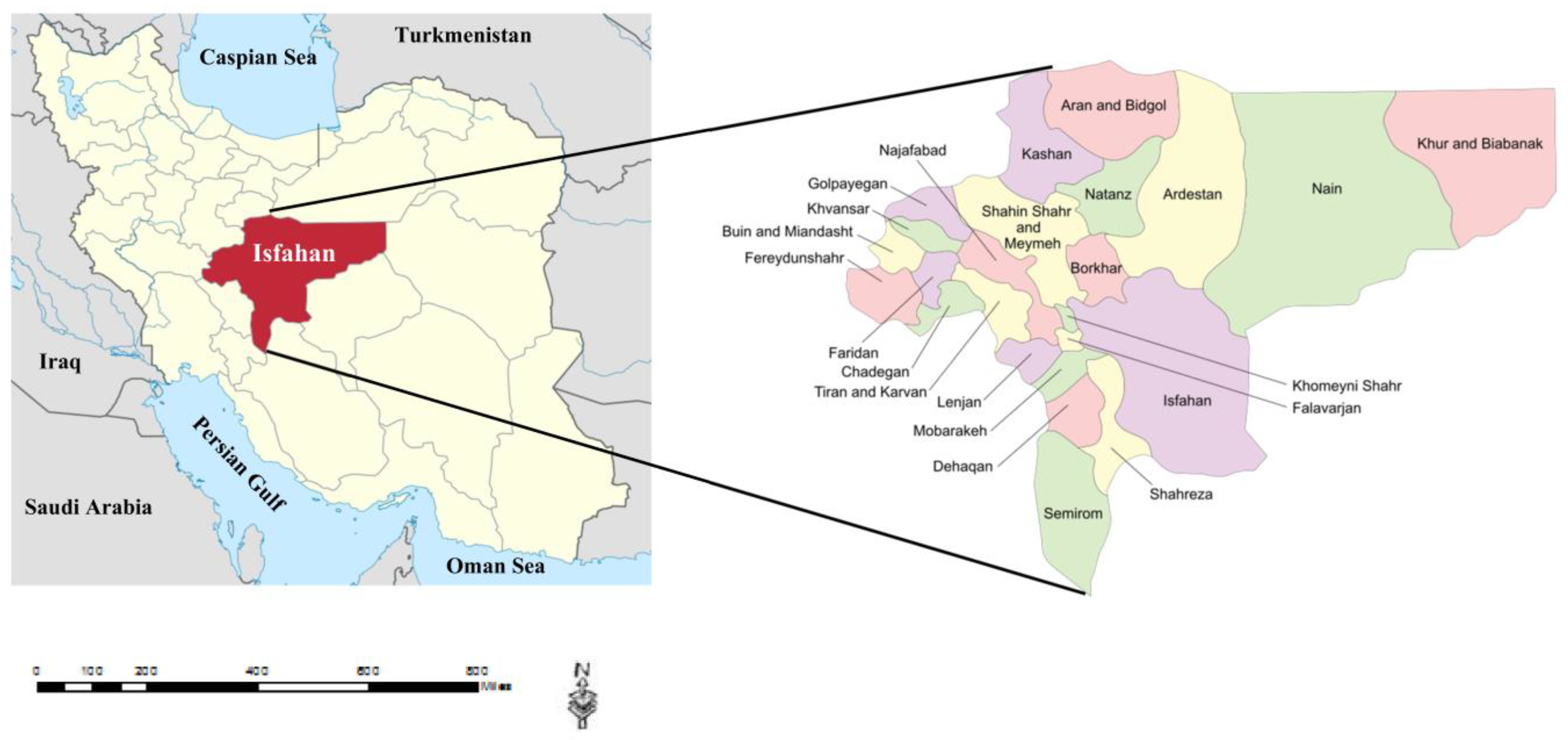
The current study follows our past studies that were performed on energy use pattern and optimization in Isfahan province, Iran, [49,50] that is illustrated in Figure 1. Data collected for the past studies are used to perform the present research.

2.2. LCA Approach

LCA is a useful and appropriate approach to assess environmental impact of agricultural production [51]. LCA structure includes four steps that contribute to a united approach [52]: (i) scope and goal definition required for the determination of functional unit (FU) and system boundaries; (ii) life cycle inventory (LCI) composed of a detailed collection of all inputs or materials used in different processes and also total pertinent outputs (pollution to water, soil, or air) in various steps of the entire life cycle; (iii) life cycle impact assessment (LCIA) goals in order to quantify the relevant importance of entire environmental harmful effects that are recognized in LCI; and (iv) result interpretation step, in which the evaluation of results are undertaken to offer suggestions and conclusions based on prior computations.
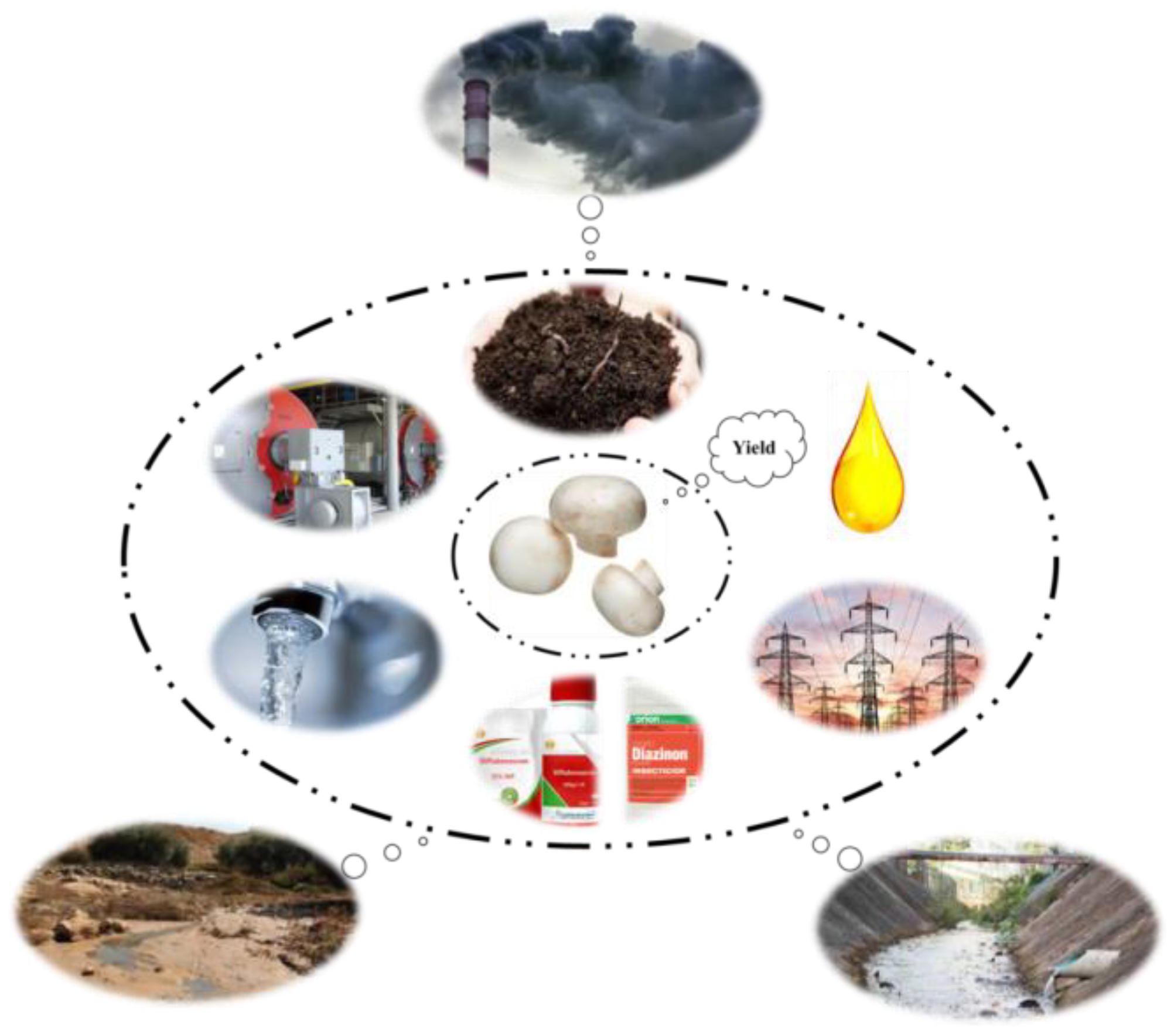
The scope and goal definition present the product system explanation in terms of FU and system boundaries [53]. According to UNI EN ISO 14040, the reference unit that quantifies the performance of a system in LCA is defined as FU [54]. In the current study, FU is defined as 100 t of mushroom production (100 TMP). In LCA, the determination of system boundaries is an important step [55]. The selection of system boundaries is a critical and major measure at this phase because any change in a boundary may affect LCA results [56]. Typical system boundaries in mushroom greenhouses include operation composting, spawning, casing, pinning, and harvesting. In Figure 2, an overview of system boundaries for mushroom production is illustrated.

2.2.1. LCI

LCI analysis is the second step of LCA. It includes collecting inventory and merging primary data (gathered for the study) and secondary data (accessible from international databases) [57]. Inventory is divided into three main sections in this research. The first part is Off-Farm emissions, which include physical values of used inputs, emissions that are results of production processes or processing performed on those inputs. The second part is On-Farm emissions, which comprise the release of inputs in the system. It should be noted that only some inputs have On-Farm emissions. In mushroom production, On-Farm emissions include:
(a)
Emissions derived from diesel fuel combustion in boilers to air and water, the standard coefficients of which are extracted based on the U.S. LCA database [58].
(b)
Emissions derived from compost consumption in the farm to air, water, and soil, for which the standard coefficients reported in previous studies were used [59,60,61].
(c)
Emissions derived from human activity to air, which is about 0.7 kg CO2 eq. per hour [62].
(d)
Emissions derived pesticides to air and water based on the PestLCI 2.0 model. PestLCI is an appropriative inventory model [63]. It should be noted that this method does not cover emissions to soil derived from pesticides. As such, the standard coefficient of emissions to soil by Margni et al. [64] was applied for this research. The last part of inventory includes the product, which is mushroom yield in this study.

2.2.2. LCIA

In LCIA, environmental impacts are evaluated, and their potential and importance are identified [65]. In studies conducted in different regions of the world, several models and methodologies have been used to develop LCIA stages [37,38,41,66]. In the present study employing SimaPro software, the ReCiPe2016 method is applied to estimate the life cycle environmental effects of mushroom production. This model determines indicators at seventeen midpoint and three endpoint levels [67].
Weighting as a final and optional phase in life LCIA is subjective and implies a value judgment, which may influence the results of LCA. Weighting shows the relative importance of the impact category [68]. According to its practicability for comparing impacts of different scenarios or products and supporting decision-making and result communication, it is commonly applied in research [69].

2.3. CExD

The sum of all source exergy required to provide a product or process, which is used for quantifying the entire life cycle exergy demand of a process or product, is called CExD [9]. For a certain process or system, exergy is described as the maximum value of work that can be obtained from the system in the process to balance with its surrounding environment [70]. CExD includes seven forms of energy.

2.4. ESC Analysis

ESC determines the external cost of burning environmental emissions. Therefore, pricing environmental emissions at its full social cost needs an estimate of ESC [71]. Quantification of ESC is necessary for policymakers to formulate emissions tax [72]. ESC was started in Iran in 2010 by Power Ministry of Iran, and its focus is mostly on electricity. All taxes on emissions are determined according to the same internal standard. In fact, the Iranian government has set the average amount of emissions of different environmental indices per kWh and considered the dollar equivalent to remove their effects from society. Environmental indices and coefficients related to their cost computations [73] that are used in this research are shown in Table 2.

2.5. ML Models

Based on the historical training data, ML models are able to customize an algorithm that recognizes the main patterns of potentially instable organizations and enables them to be recognized [74]. ML algorithms handle a variety of input data of different types and scales without any need for pre-defined data structure. There are several algorithms for modeling in different research areas. The most widely used ML algorithms are ANN, ANFIS, and SVR, which are explained briefly in the following sections.

2.5.1. Development of ANN Model

ANN, as a basic tool applied in ML, is a computational and simulation model based on the biological nodal cell structure, designed to simulate the way that human brain processes and analyzes information [75]. ANN is able to construct a model relating the output of network to existing data used as inputs. The structure of ANN includes three layers, namely an input layer to take actual data, one or several hidden layers to link input and output layers, and an output layer to produce computed results [76].
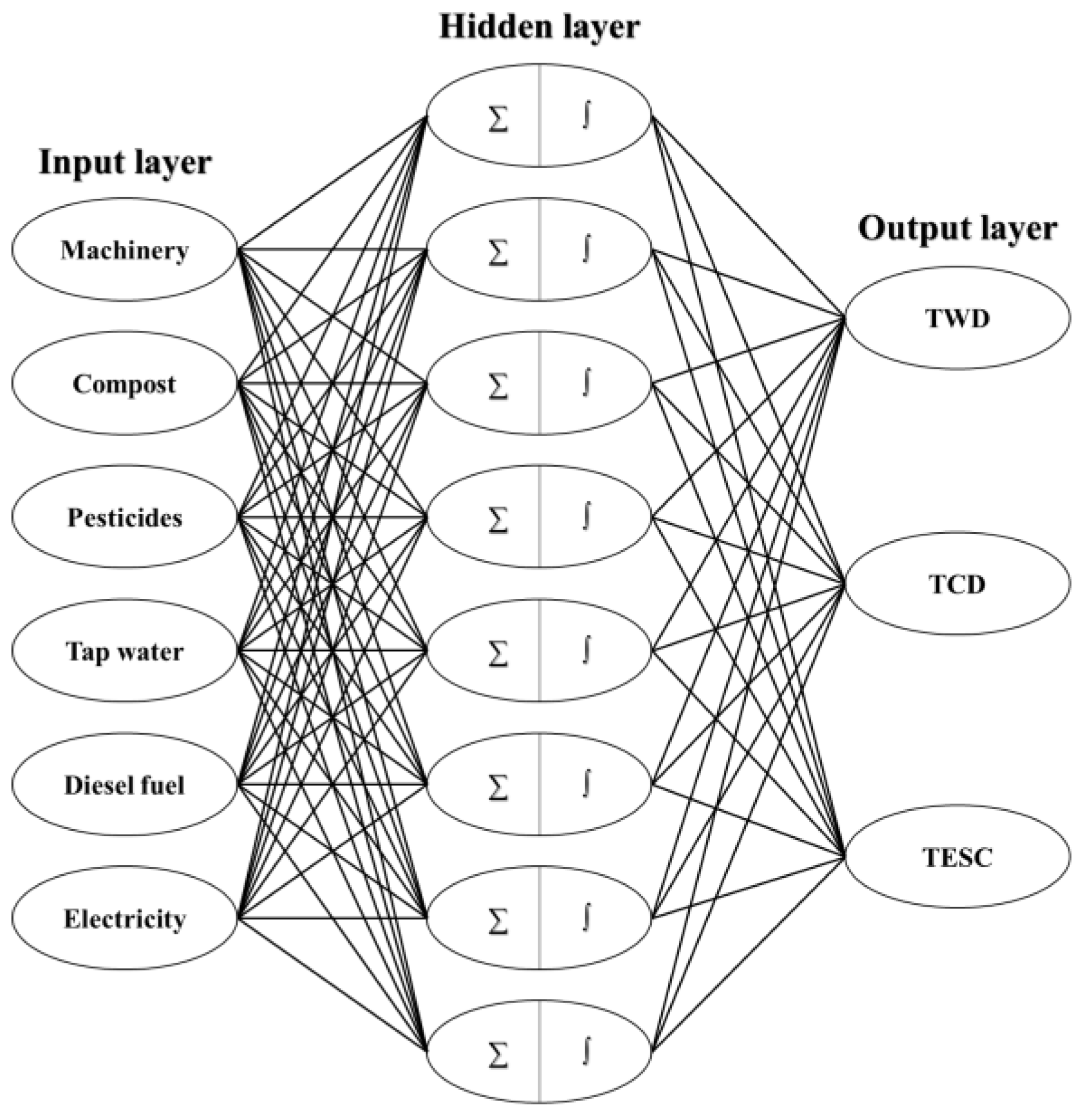
In this study, a back-propagation feed-forward ANN with one input layer, one to three hidden layers, and one output layer was applied for estimating total weighted damages (TWD), total cumulative exergy demand (TCD), and total emissions social cost (TESC) of button mushroom production from the collected actual data. The input layer consists of six independent variables (machinery, compost, pesticides, tap water, diesel fuel, and electricity) while the output layer includes 3 dependent variables (TWD, TCD, and TESC), and different numbers of hidden layers with different neuron numbers are adopted to find the best structure. Of this data, 75, 15, and 10% are utilized for training, testing, and cross-validation of the network, respectively. Among different algorithms in ANN, the Levenberg–Marquardt algorithm with an early stopping criterion to enhance the efficiency and speed of network training is good at solving continuous modeling problems [77]. In computing and mathematics, the Levenberg–Marquardt algorithm, also called the damped least-squares method, is applied to solve non-linear least squares cases [78]. Accordingly, the Levenberg–Marquardt algorithm is selected to apply in ANN model of this study.
The differences between the computed results and observed data are utilized for the evaluation of ANN model performance. The error function utilized in the performance evaluation is given by Equation (1) [79]:
E = 1 p p k ( t p k z p k ) 2
where k indicates the output vector index; p represents the input vectors index; tpk denotes the kth element of the pth vector of the target pattern; and zpk is the kth output vector element under input pattern p.

2.5.2. Development of ANFIS Model

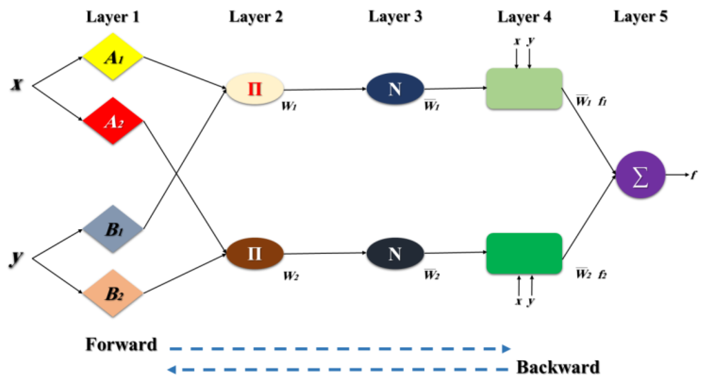
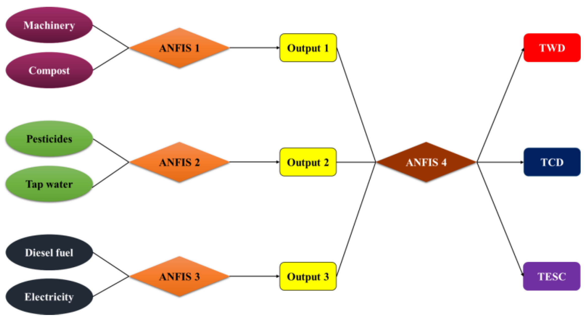
Fuzzy logic, as an artificial simulation technique, develops a numeric method using if/then rules and permits for the simple display of production process knowledge [80]. ANFIS is an ML method that merges fuzzy logic theories and adaptive ANN rules to constitute an adaptive network to make a reasonable relation between outputs and inputs [81]. With the ANN method, the ANFIS model is expanded by data trained or learned [82]. A schematic of the ANFIS model is shown in Figure 3, illustrating two inputs (A; B) and one output (Si) in this model. Because of the large number of inputs for ANFIS, firstly the input vector is divided into three categories. Figure 4 presents the two-level ANFIS structure used in this study to predict the TWD, TCD, and TESC of mushroom production.

2.5.3. Development of SVR Model

The basic purpose of SVR is to exactly match a regression function y = f(x) in a ε-SVR model for objects {yi} regarding a collection of input data {xi} by training data as D = {(x1, y1), (x2, y2), …, (xN, yN)}, where xi ∈ RN is an input variables vector, and yi ∈ RN is the scalar target value. In the real world and for non-linear issues, when it is not possible for input data to correlate linearly to the required output, a linear model can be created utilizing a nonlinear mapping function gi(x) in high-dimensional feature space as shown in Equation (2).
f ( X , ω ) = i = 1 n ω i g i ( X )   + b
where gi(x) is the function termed feature, and ωi.gi(x) is the dot product in the feature space F, and b is the bias. It acts based on minimizing structural risk law [83]. Using the minimizing risk function, the coefficients can be estimated as:
R ( C ) = C 1 l i = 1 l L c ( y i , f ( X i , ω ) ) + 1 2 ω 2
The risk function (Equation (3)) consists of two parts, namely an empirical error term  C 1 l i = 1 l L c ( y i , f ( X i , ω ) ) and a smoothness or flatness function  1 2 ω 2 . The empirical error part includes a function ε insensitive loss function  L c ( y i , f ( X i , ω ) ) and a factor C.
L c ( y i , f ( X i , ω ) ) = y f ( ω ) | ε , f o r | y f ( X , ω ) | ε 0 , f o r | y f ( X , ω ) | ε
where C is a measure of the trade-off amount among the flatness of model and the empirical error. Slack variables  ξ , ξ * , as positive constants, are determined to compute errors exceeding the limit ε. Using slack variables, the SVR problem is converted into a dual optimization problem whose objective function is:
Minimization   of z ( ω , b , ξ , ξ * ) = 1 2 ω 2 + C i = 1 l ( ξ i + ξ i ) Subjected   to   constraint   equation y i f ( X i , ω ) ε + ξ i f ( X i , ω ) y i ε + ξ i ξ i , ξ i 0
In order to solve the problem of convex optimization, the Lagrangian multiplier method is applied. The transformed formula with the multipliers is expressed as follows:
f ( X , α i , α i ) = i = 1 N ( α i α i ) ( g ( X i ) . g ( X j ) ) + b
where αi and αi* are the Lagrangian multipliers. The input vectors xi are termed support vectors provided that their corresponding coefficients (αiαi*) ≠ 0. These vectors are the representative of the entire support vector function because they comprise most of the training data set information. In order to overcome the contradiction among the complexity in computation and the high dimensional featured space, an appropriate kernel function must be determined [83]. Each function that is positive, symmetric, and semi-definite (Mercer’s condition) can be considered as a kernel function [84]. The Gaussian radial basis function (RBF) is the most commonly used kernel function, which is described as follows [85,86]:
K ( X i , X j ) = ( g ( X i ) g ( X j ) ) = exp ( 1 2 σ 2 X i X j 2 ) = exp ( γ X i X j 2 ) w h e r e , i , j = 1 , , N
where σ is the RBF width, and γ is equal to 1/(2σ2).
Therefore, all computations about g can be performed by an explicit method within the input space itself using the kernel function, without really bothering the featured space. The basic formula explaining the data modeling is as follows:
f ( X , α i , α i ) = i = 1 N ( α i α i ) ( K ( X i , X j ) + b )
Using Karush–Kuhn–Tucker conditions, the parameter b can be determined as:
b = 1 2 i = 1 N ( α i α i ) g [ ( X m , X i ) + K ( X n , X i ) ]
where xm and xn are the support vectors.
For optimizing the model parameters C = 100 and ε = 0.001 and the RBF kernel parameter γ = 0.3, the grid search method in connection with 10 folds-cross validation is applied. The model parameters C and e and the kernel parameter c are variables in the ranges of (22–215), (2−10–25), and (2−10–24), respectively. It should be noted that in all models the number of support vector was 89, and the number of training points was 207.

2.5.4. Evaluation of Model Performance

In order to assess the efficacy of various models, statistical analysis is performed with three statistical indicators, namely absolute average relative error (AARE), root mean square error (RMSE), and coefficient of determination (R2), as follows:
A A R E = 1 n i = 1 N | [ Y P i Y A i Y A i ] |
R M S E = i = 1 N ( Y P i Y A i ) 2 n
R 2 = 1 i = 1 N ( Y P i Y A i ) 2 i = 1 N Y A i 2
where n is number of training vector; YPi is the predicted value; and YAi is the actual value.
In addition to the above statistical indicators, two other indicators are used in SVR including square correlation coefficient for leave-one-out cross-validation (Q2LOO) and square correlation coefficient of external validation (Q2EXT).
Q2LOO is a measurement of the internal prediction capability of SVR model and mostly assessed as leave one out cross-validation on the training data [86].
Q L O O 2 = i = 1 n T r a i n i n g ( Y A i Y P i ) 2 i = 1 n T r a i n i n g ( Y A i Y P i M e a n ) 2
Q2EXT is the measurement of the external prediction capability of SVR model and mostly assessed as leave one out on the test data [86].
Q E X T 2 = i = 1 n T e s t ( Y A i Y P i ) 2 i = 1 n T e s t ( Y A i Y P i M e a n ) 2
Excel V16.0 is applied to perform analysis, statistical indices computation, and analysis of ESC in this study. In addition, SimaPro V9.1.0 software is employed to implement LCA analysis as well as CExD. Finally, Python V3.9.1 is used to develop ANN and ANFIS and SVR models.

3. Results and Discussion

3.1. Environmental Analysis of Mushroom Production

The consumed inputs and resulting direct emissions for mushroom production in the studied region are illustrated in Table 3. It can be observed that the total CO2 emission discharged to the atmosphere due to utilization of diesel fuel in different mushroom production operations is 224.02 kg ha−1. The reason for this is excessive and inefficient use of diesel fuel to heat greenhouses in the region. Moreover, different stages of compost production and consumption lead to the release of 945.091 t ha−1 of CO2. Inefficient usage of diesel fuel in mushroom production has different reasons including old systems of heating equipment, high heat losses of greenhouses, and old methods of compost production.
In the production process of compost, diesel fuel is used to supply heating required by microorganisms. It is also used in the mushroom production process to maintain the greenhouse temperature in optimal conditions. Low diesel fuel price in Iran, which leads to its inefficient use in various industries, is one of the reasons of high diesel fuel consumption. Heating systems used in mushroom greenhouses have low efficiency and consume large amounts of fossil fuels due to the lack of intelligent heating system.
Thus, to reduce diesel fuel consumption and mitigate its negative effects, it is recommended that high efficiency heating systems with less pollution are to be applied. Insulation of greenhouse walls and the use of materials with low heat transfer coefficient in the construction of greenhouse walls and roofs can also be useful in preventing heat loss. These strategies also reduce the energy consumption required for fuel transportation. Natural gas is less polluting than diesel fuel, and given that Iran is rich in natural gas resources, the use of natural gas to provide heating in mushroom production is recommended as an early return strategy.
Dorr et al. [87] studied the environmental effects of an urban mushroom farm in France. They reported that in terms of climate change impact, the product system emitted about 3 kg CO2-eq. kg−1 mushroom, and On-Farm energy consumption was the top contributor to all impact categories.
Endpoint results by applying LCA method for 100TMP are illustrated in Table 4. Human health damage category is 0.91 DALY per 100TMP. DALY is an overall measure of disease burden, defined as the number of years lost because of disability, early death, or ill-health. It is introduced as a method to compare the life expectancy and overall health (Table 4).
Hosseini-Fashami et al. [40] investigated environmental effects of strawberry production and reported that human health per 100 t of greenhouse strawberry production was 0.097 DALY. Mostashari-Rad et al. [46] studied environmental indicators for horticultural crops and reported these indicators as 0.5 and 0.1 for 100 t of hazelnut and citrus production, respectively.
Resources and ecosystems are other damage categories, which are determined by the ReCiPe2016 method. As can be seen in Table 4, ecosystem damage category is 2.84 × 10⁻³ species.yr per 100TMP. Moreover, resources damage category is computed as 35,850.42 USD2013 based on FU.
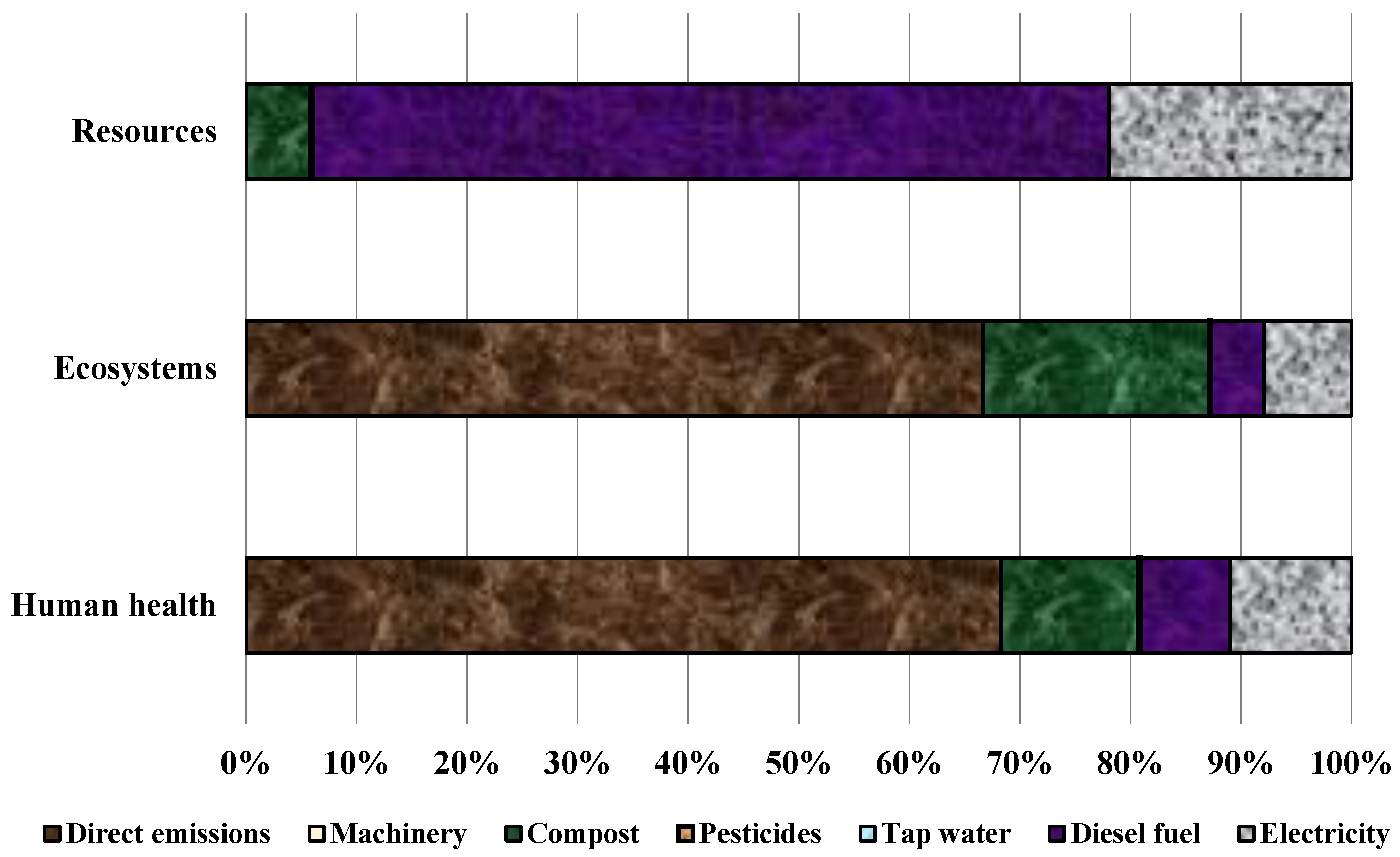
Figure 5 shows the pattern of environmental impacts and contribution of various inputs to mushroom production endpoints. The highest effect in ecosystems and human health damage categories is direct emissions. Direct emissions are related to input consumption in the production process of mushroom. Irregular diesel fuel use in compost production is one of the most important factors on direct emissions. Based on these results, the greatest effects in resources damage category is from diesel fuel. This shows that in mushroom production, diesel fuel consumption brings great loss on environment, and its usage must be decreased to diminish environmental risk. Electricity is another input that has significant effect on resources damage categories. In greenhouses, electricity is used for lighting, electric equipment, and sometimes for heating. Low efficiency of production and transmission network of electricity as well as use of time-worn electrical equipment are reasons for high electricity consumption in the studied greenhouses.
Comparison between the greenhouses and farms indicated that the greenhouses have more severe detrimental effects on environmental impacts. Fossil fuels are one of the most important items for this result. With respect to the geographical position of studied area, replacing renewable technologies especially solar systems can be an appropriate solution to improve the environmental damage. Moreover, ground air collectors using phase change materials are the cheapest and most popular methods during application of solar systems.
In several studies similar results were reported that direct emissions had the greatest effect in ecosystem and human health damage categories [44,46,88,89].
Because of different units of investigated damage categories, it is not possible to compare them with one another. Thus, to overcome this problem, a weighting method is applied. The weighting results demonstrated that, among three damage categories, human health with about 15 kPt, is significantly category from the emission viewpoint. Direct emissions (more due to diesel fuel consumption) have the greatest contribution in this category, followed by compost. Ecosystems index is at the next place, and the share of direct emissions is a major part of this impact.
Hosseini-Fashami et al. [40] used weighting analysis to compare damage categories in greenhouse strawberry production and reported that from the emission viewpoint, ecosystem quality is the major category.

3.2. Energy Form Assessment of CExD

The energy assessment results according to CExD in mushroom greenhouses are shown in Table 5. The results demonstrate that TCD of mushroom production is about 3974 GJ 100 TMP−1. The category of non-renewable, fossil is the highest form of energy consumption in mushroom production (about 98% of TCD). The non-renewable fossil value is computed as 7088.05 GJ 100 TMP−1 (Table 5). In the mushroom production system, fossil fuel usage is for heating propose, and because its utilization is high, this results in high non-renewable, fossil form utilization in this system.
In a study carried out in northwest of Iran, Nabavi-Pelesaraei et al. [90] employed CexD for energy assessment of oil production from sunflowers. Their results demonstrated that the category non-renewable fossil was about 173,499 MJ per one t of sunflower oil production.
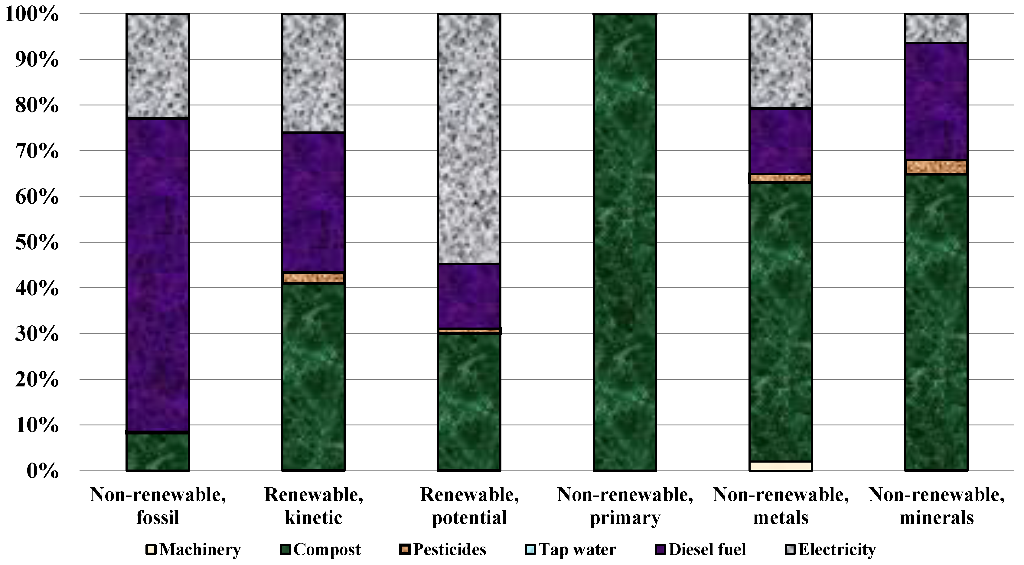
The percentages of different input energy forms of CExD for mushroom greenhouses are illustrated in Figure 6. The results show that, in mushroom production, diesel fuel has the largest percentage of share in the category non-renewable, fossil (around 70%) and is followed by electricity (about 23%). Similar results have been reported in many studies conducted in Iran where diesel fuel is the main factor in the category non-renewable, fossil [17,44]. The results also indicate that, in non-renewable, potential, electricity has the greatest energy usage among different inputs. Furthermore, in non-renewable, primary, non-renewable, minerals, non-renewable, meals, and renewable, kinetic, compost has the highest energy usage among different inputs. This displays that a large amount of inputs are used inefficiently in compost production. Thus, a proper usage of inputs, especially diesel fuel in compost production, can result in great energies reduction for mushroom production.

3.3. Evaluation of ESC

The results of ESC for 100 TMP are shown in Table 6. The results indicate that TESC per 100 TMP in Isfahan province is equal to 1035.10$, in which a large part is related to ESC of CO2, SO2, and NOX. In other words, the shares of CO2, SO2, and NOX are equal to 47.1, 37.3 and 11% of TESC, respectively. In another study about ESC of agricultural systems, Nabavi-Pelesaraei et al. [42] estimated TESC for rice milling factories was about 31$ per t of white rice in the Guilan province of Iran. Their results also showed that a large part of this cost is related to CO2 emission.
The high consumption of diesel fuel in mushroom production can also be considered in terms of TSC. Compared to other emissions, the unit cost of CO2 is small; nevertheless, due to high utilization of diesel fuel in mushroom production which leads to high emission of CO2, it will be one of the major portions of the whole cost. Therefore, saving diesel fuel consumption can reduce TESC in mushroom production. Besides, a change in fuel type used in compost production process and the application of renewable energy are strongly recommended.

3.4. ANN Model Assessment

In the current study, a back-propagation feed-forward ANN was used for estimating TWD, TCD, and TESC of button mushroom production. For all models, statistical metrics including R2, AARE, and RMSE were computed. The schematic diagram of the best structure of ANN model by the maximum R2 and lowest AARE and RMSE values is presented in Figure 7. As shown in Figure 7, the structure with one hidden layer is the best ANN structure in all models (6-8-3).
The statistical indicators of the ANN models in TWD, TCD, and TESC of mushroom production are listed in Table 7. The results indicate that, for mushroom production, R2 ranges from 0.889 to 0.915 for the training stage, 0.886 to 0.912 for the testing stage, and 0.893 to 0.927 overall. The results also demonstrate that R2 ranges from 0.881 to 0.911 in the validation stage. This indicate that the introduced model is able to forecast TWD, TCD, and TESC in mushroom production.
High accuracy of ANN models was recognized in some previous researches such as Bai et al. [91] for forecasting air pollutants concentrations, Gao et al. [92] for estimation of ozone concentration, Acheampong and Boateng [93] for modeling carbon emission intensity, and Gonçalves Neto et al. [94] for modeling of biogas production from food.

3.5. ANFIS Model Assessment

Statistical components of the two-level ANFIS structure in predicting TWD, TCD, and TESC of mushroom production are shown in Table 8. According to results, ANFIS with Gbell MFs for input layer and linear MF for output layer offers the best performance. In other words, this hybrid learning method can simulate the communication among inputs and outputs, specify the optimized MF contribution, and provide great precision.
The two-level ANFIS model (ANFIS 4) is shown in the results, with the highest R2 found for TESC (0.872). In this model, the RMSE is computed as 0.219. The results also show that, in the two-level ANFIS model (ANFIS 4), R2 for TCD is 0.870, and AARE is 6.57. Results of the current study agree with Kaab et al. [18], which applied ANFIS to forecast output energy and environmental effects of sugarcane cultivation. Naderloo et al. [19] used ANFIS model for forecasting of wheat grain yield in Iran. They clustered the inputs for ANFIS into two categories and trained two networks. Electricity, diesel fuel, and chemical fertilizer energies were inputs for ANFIS 1, and machinery, labor, chemicals, water, and seed energies were considered for ANFIS 2. Their RMSE values were 0.013 and 0.018 for ANFIS1 and ANFIS 2, respectively. Besides, R2 values were 0.996 and 0.992 for ANFIS 1 and ANFIS 2, respectively. Finally, they used these predicted values as the inputs of the third ANFIS and found that RMSE and R2 were 0.013 and 0.996, respectively.

3.6. SVR Model Assessment

The performance parameters including AARE, RMSE, Q2LOO, and Q2EXT are tabulated in Table 9. The ranges of RMSE, Q2LOO, and Q2EXT AARE are between 0.85 and 1.03, between 0.003 and 0.011, between 0.161 and 0.179, and between 0.233 and 0.252 for TWD, TCD, and TESC, respectively. The results of performance parameters reveal that the accuracy of SVR model is very high. Other studies on application of SVR in agri-industrial modeling confirmed the results in attaining high accuracy for predicting different parameters [95,96,97].

3.7. Comparison between Evaluated ML Models

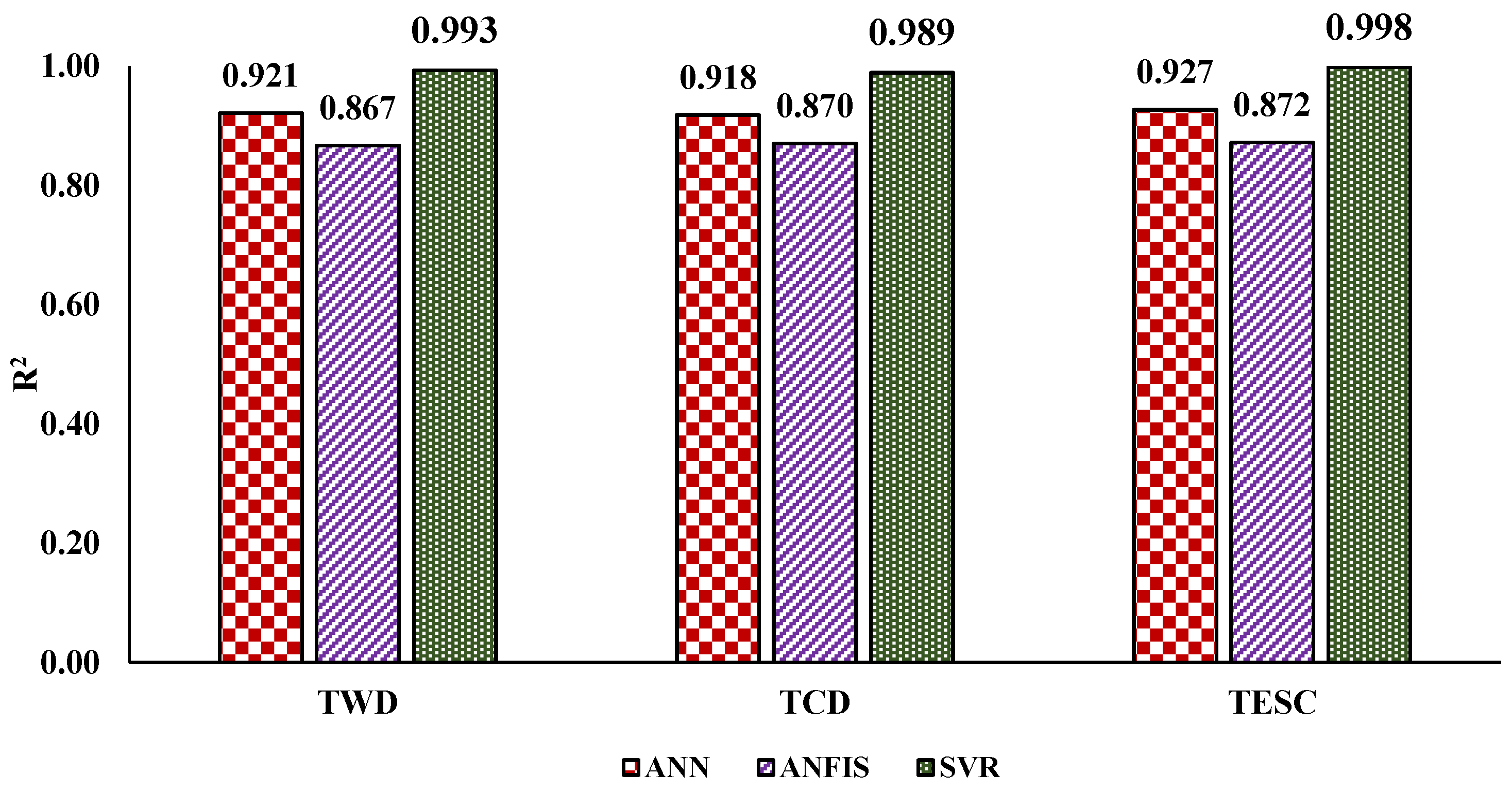
In the last section, the accuracies of different ML models are evaluated using coefficients of determination. Figure 8 shows R2 in different ML models, which indicates that the R2 of the SVR model for predicting dependent variables including TWD, TCD, and TESC are higher than the R2 of other models. In other words, SVR model outperforms other models. Taheri et al. [98] applied ANN and SVR to model the drying of lentil in a microwave fluidized bed. The results indicated that moisture ratio and temperature of lentil could be predicted accurately using ANN and SVR. Performance evaluation of the models with statistical parameters indicated that ANN provided relatively better accuracy for prediction of lentil temperature.
Comparison of results between ANN and ANFIS shows that the ANN model outperforms the ANFIS model. In studies that used ANN and ANFIS for prediction, different results have been reported. Depending on the type of data and the model case, one of these two methods had better performance. In research performed by Kaab et al. [18], ANFIS and ANN models were used to forecast energy output and environmental issue of sugarcane farms. The results showed that in the plant farms, ANN was better than ANFIS in all dimensions, but in the case of ratoon farms, the results were different, and ANFIS achieved better prediction results than ANN.
Modeling results indicated that SVR had the highest performance for prediction environmental damages, exegetic categories, and ESC with respect to statistical indicators. In this sense, SVR models are more user-friendly, need less computation, and can use multiple classifiers trained on various types of data. On the other hand, ANN can develop better models in comparison. A low uncertainty rate in greenhouses production is the main reason for this result. Finally, it is advised that more research such as optimization with multi-objective approach (environmental, energy and economical) of mushroom production will be used for improving environmental condition.

4. Conclusions

The current study investigates the applications of different ML methods including ANN, ANFIS, and SVR for modeling environmental impacts, exergy categories, and emissions social cost (ESC) of mushroom production. According to results of the current study, the following conclusions can be drawn:
  • In general, in human health and ecosystem damage categories, direct emissions have the highest portion. Furthermore, in resources damage category, diesel has the most significant impact.
  • Diesel fuel and electricity have the highest and second highest portions in the categories of Non-renewable, fossil, respectively. In Non-renewable, primary, Non-renewable, metals, Non-renewable, minerals, and Renewable, kinetic, compost has a high share among energy consumption of inputs.
  • ESC results indicate that TESC per 100TMP is 1035.10$, in which a large part is related to ESC of CO2, SO2, and NOX.
  • Results of ANN model show that 6-8-3 topology is the best structure for predicting TWD, TCD, and TESC.
  • The best model of ANFIS that attains the highest accuracy is obtained by a two-level structure with Gbell MFs for input layer and linear MF for output layer.
  • SVR modeling reveals that statistical indices including AARE (%), RMSE, and R2 vary in ranges of 0.85–1.03, 0.003–0.011, and 0.989–0.993 for TWD, TCD, and TESC, respectively.
  • Comparison between the investigated ML models indicates that the SVR model outperforms others models in predicting TWD, TCD, and TESC. Moreover, the accuracy of ANN model is better than ANFIS. The reason of this result is the certainty of data in mushroom production in the studied area.
Finally, it should be noted that, although the prediction of exergoenvironmental index and ESC can be useful to save time and costs by ML methods, it is recommended to focus on optimization methods for enhancement of input consumption efficiency and reduction of negative exergoenvironmental effects of mushroom production for future studies.
Author Contributions

Conceptualization, A.N.-P.; Data curation, M.S.; Formal analysis, A.N.-P. and H.G.-M.; Investigation, R.E.; Methodology, A.N.-P.; Project administration, A.N.-P. and R.E.; Software, S.R.; Supervision, A.N.-P., H.G.-M. and R.E.; Writing—original draft, A.N.-P. and H.G.-M.; Writing—review and editing, A.N.-P., H.G.-M. and K.-W.C. All authors have read and agreed to the published version of the manuscript.

Funding

This research received no external funding.

Informed Consent Statement

Informed consent was obtained from all subjects involved in the study.

Data Availability Statement

The original contributions presented in the study are included in the article.

Acknowledgments

We gratefully acknowledge the financial support provided by Department of Agricultural Machinery Engineering, Faculty of Agricultural Engineering and Technology, University of Tehran, Karaj, Iran.

Conflicts of Interest

The authors declare that the research was conducted in the absence of any commercial or financial relationships that could be construed as a potential conflict of interest.

References

  1. Beelman, R.; Royse, D.; Chikthimmah, N. Bioactive Components in Button Mushroom Agaricus Bisporus (J. Lge) Imbach (Agaricomycetideae) of Nutritional, Medicinal, and Biological Importance (Review). Int. J. Med. Mushrooms 2003, 5, 321–337. [Google Scholar] [CrossRef]
  2. Food and Agriculture Organization (FAO). 2022. Available online: http://www.fao.org (accessed on 17 March 2022).
  3. Ministry of Jihad-e-Agriculture of Iran Annual Agricultural Statistics. 2021. Available online: www.maj.ir (accessed on 21 November 2021). (In Persian).
  4. Pathak, H.; Wassmann, R. Introducing Greenhouse Gas Mitigation as a Development Objective in Rice-Based Agriculture: I. Generation of Technical Coefficients. Agric. Syst. 2007, 94, 807–825. [Google Scholar] [CrossRef]
  5. Ghorbani, R.; Mondani, F.; Amirmoradi, S.; Feizi, H.; Khorramdel, S.; Teimouri, M.; Sanjani, S.; Anvarkhah, S.; Aghel, H. A Case Study of Energy Use and Economical Analysis of Irrigated and Dryland Wheat Production Systems. Appl. Energy 2011, 88, 283–288. [Google Scholar] [CrossRef]
  6. Guinée, J.B.; Heijungs, R.; Huppes, G.; Zamagni, A.; Masoni, P.; Buonamici, R.; Ekvall, T.; Rydberg, T. Life Cycle Assessment: Past, Present, and Future. Environ. Sci. Technol. 2011, 45, 90–96. [Google Scholar] [CrossRef]
  7. Strazza, C.; Del Borghi, A.; Gallo, M.; Del Borghi, M. Resource Productivity Enhancement as Means for Promoting Cleaner Production: Analysis of Co-Incineration in Cement Plants through a Life Cycle Approach. J. Clean. Prod. 2011, 19, 1615–1621. [Google Scholar] [CrossRef]
  8. Lal, R. Carbon Emission from Farm Operations. Environ. Int. 2004, 30, 981–990. [Google Scholar] [CrossRef] [PubMed]
  9. Khanali, M.; Ghasemi-Mobtaker, H.; Varmazyar, H.; Mohammadkashi, N.; Chau, K.W.; Nabavi-Pelesaraei, A. Applying Novel Eco-Exergoenvironmental Toxicity Index to Select the Best Irrigation System of Sunflower Production. Energy 2022, 250, 123822. [Google Scholar] [CrossRef]
  10. Peters, J.F.; Petrakopoulou, F.; Dufour, J. Exergetic Analysis of a Fast Pyrolysis Process for Bio-Oil Production. Fuel Process. Technol. 2014, 119, 245–255. [Google Scholar] [CrossRef]
  11. Stoellinger, T.; Righetti, T.; Coddington, K. Impact of Social Cost of Carbon Analyses in the Development of Energy Projects on Federal Land. Electr. J. 2016, 29, 63–70. [Google Scholar] [CrossRef]
  12. Vadiee, A.; Martin, V. Energy Management in Horticultural Applications through the Closed Greenhouse Concept, State of the Art. Renew. Sustain. Energy Rev. 2012, 16, 5087–5100. [Google Scholar] [CrossRef]
  13. Tian, L.; Ye, Q.; Zhen, Z. A New Assessment Model of Social Cost of Carbon and Its Situation Analysis in China. J. Clean. Prod. 2019, 211, 1434–1443. [Google Scholar] [CrossRef]
  14. Hosseinzadeh-Bandbafha, H.; Safarzadeh, D.; Ahmadi, E.; Nabavi-Pelesaraei, A.; Hosseinzadeh-Bandbafha, E. Applying Data Envelopment Analysis to Evaluation of Energy Efficiency and Decreasing of Greenhouse Gas Emissions of Fattening Farms. Energy 2017, 120, 652–662. [Google Scholar] [CrossRef]
  15. Ao, Y.; Li, H.; Zhu, L.; Ali, S.; Yang, Z. The Linear Random Forest Algorithm and Its Advantages in Machine Learning Assisted Logging Regression Modeling. J. Pet. Sci. Eng. 2019, 174, 776–789. [Google Scholar] [CrossRef]
  16. Wuest, T.; Weimer, D.; Irgens, C.; Thoben, K.-D. Machine Learning in Manufacturing: Advantages, Challenges, and Applications. Prod. Manuf. Res. 2016, 4, 23–45. [Google Scholar] [CrossRef] [Green Version]
  17. Fernández-Delgado, M.; Cernadas, E.; Barro, S.; Amorim, D. Do We Need Hundreds of Classifiers to Solve Real World Classification Problems? J. Mach. Learn. Res. 2014, 15, 3133–3181. [Google Scholar]
  18. Nabavi-Pelesaraei, A.; Rafiee, S.; Mohtasebi, S.S.; Hosseinzadeh-Bandbafha, H.; Chau, K.W. Integration of Artificial Intelligence Methods and Life Cycle Assessment to Predict Energy Output and Environmental Impacts of Paddy Production. Sci. Total Environ. 2018, 631–632, 1279–1294. [Google Scholar] [CrossRef]
  19. Kaab, A.; Sharifi, M.; Mobli, H.; Nabavi-Pelesaraei, A.; Chau, K.W. Combined Life Cycle Assessment and Artificial Intelligence for Prediction of Output Energy and Environmental Impacts of Sugarcane Production. Sci. Total Environ. 2019, 664, 1005–1019. [Google Scholar] [CrossRef]
  20. Naderloo, L.; Alimardani, R.; Omid, M.; Sarmadian, F.; Javadikia, P.; Torabi, M.Y.; Alimardani, F. Application of ANFIS to Predict Crop Yield Based on Different Energy Inputs. Measurement 2012, 45, 1406–1413. [Google Scholar] [CrossRef]
  21. Hou, Q.; Zhang, J.; Liu, L.; Wang, Y.; Jing, L. Discriminative Information-Based Nonparallel Support Vector Machine. Signal Process. 2019, 162, 169–179. [Google Scholar] [CrossRef]
  22. Wang, J.; Shan, Y.; Xie, X.; Kuang, J. Output-Based Speech Quality Assessment Using Autoencoder and Support Vector Regression. Speech Commun. 2019, 110, 13–20. [Google Scholar] [CrossRef]
  23. Mobtaker, H.G.; Keyhani, A.; Mohammadi, A.; Rafiee, S.; Akram, A. Sensitivity Analysis of Energy Inputs for Barley Production in Hamedan Province of Iran. Agric. Ecosyst. Environ. 2010, 137, 367–372. [Google Scholar] [CrossRef]
  24. Boulard, T.; Raeppel, C.; Brun, R.; Lecompte, F.; Hayer, F.; Carmassi, G.; Gaillard, G. Environmental Impact of Greenhouse Tomato Production in France. Agron. Sustain. Dev. 2011, 31, 757–777. [Google Scholar] [CrossRef] [Green Version]
  25. Ozkan, B.; Ceylan, R.F.; Kizilay, H. Energy Inputs and Crop Yield Relationships in Greenhouse Winter Crop Tomato Production. Renew. Energy 2011, 36, 3217–3221. [Google Scholar] [CrossRef]
  26. Taki, M.; Mahmoudi, A.; Ghasemi Mobtaker, H.; Rahbari, H.; Mobtaker, H.G.; Rahbari, H. Energy Consumption and Modeling of Output Energy with Multilayer Feed-Forward Neural Network for Corn Silage in Iran. Agric. Eng. Int. CIGR J. 2012, 14, 93–101. [Google Scholar]
  27. Hakala, K.; Nikunen, H.M.; Sinkko, T.; Niemeläinen, O. Yields and Greenhouse Gas Emissions of Cultivation of Red Clover-Grass Leys as Assessed by LCA When Fertilised with Organic or Mineral Fertilisers. Biomass Bioenergy 2012, 46, 111–124. [Google Scholar] [CrossRef]
  28. Abeliotis, K.; Detsis, V.; Pappia, C. Life Cycle Assessment of Bean Production in the Prespa National Park, Greece. J. Clean. Prod. 2013, 41, 89–96. [Google Scholar] [CrossRef]
  29. Soni, P.; Taewichit, C.; Salokhe, V.M. Energy Consumption and CO2 Emissions in Rainfed Agricultural Production Systems of Northeast Thailand. Agric. Syst. 2013, 116, 25–36. [Google Scholar] [CrossRef]
  30. Sefeedpari, P.; Rafiee, S.; Akram, A.; Komleh, S.H.P. Modeling Output Energy Based on Fossil Fuels and Electricity Energy Consumption on Dairy Farms of Iran: Application of Adaptive Neural-Fuzzy Inference System Technique. Comput. Electron. Agric. 2014, 109, 80–85. [Google Scholar] [CrossRef]
  31. Romero-Gámez, M.; Audsley, E.; Suárez-Rey, E.M. Life Cycle Assessment of Cultivating Lettuce and Escarole in Spain. J. Clean. Prod. 2014, 73, 193–203. [Google Scholar] [CrossRef]
  32. Safa, M.; Samarasinghe, S.; Nejat, M. Prediction of Wheat Production Using Artificial Neural Networks and Investigating Indirect Factors Affecting It: Case Study in Canterbury Province, New Zealand. J. Agr. Sci. Tech 2015, 17, 791–803. [Google Scholar]
  33. Nabavi-Pelesaraei, A.; Rafiee, S.; Hosseinzadeh-Bandbafha, H.; Shamshirband, S. Modeling Energy Consumption and Greenhouse Gas Emissions for Kiwifruit Production Using Artificial Neural Networks. J. Clean. Prod. 2016, 133, 924–931. [Google Scholar] [CrossRef]
  34. Sefeedpari, P.; Rafiee, S.; Akram, A.; Chau, K.W.; Pishgar-Komleh, S.H. Prophesying Egg Production Based on Energy Consumption Using Multi-Layered Adaptive Neural Fuzzy Inference System Approach. Comput. Electron. Agric. 2016, 131, 10–19. [Google Scholar] [CrossRef]
  35. Chen, P.; Jing, Q. A Comparison of Two Adaptive Multivariate Analysis Methods (PLSR and ANN) for Winter Wheat Yield Forecasting Using Landsat-8 OLI Images. Adv. Space Res. 2017, 59, 987–995. [Google Scholar] [CrossRef]
  36. Fodor, N.; Challinor, A.; Droutsas, I.; Ramirez-Villegas, J.; Zabel, F.; Koehler, A.-K.; Foyer, C.H. Integrating Plant Science and Crop Modeling: Assessment of the Impact of Climate Change on Soybean and Maize Production. Plant Cell Physiol. 2017, 58, 1833–1847. [Google Scholar] [CrossRef] [PubMed] [Green Version]
  37. Mousavi-Avval, S.H.; Rafiee, S.; Sharifi, M.; Hosseinpour, S.; Shah, A. Combined Application of Life Cycle Assessment and Adaptive Neuro-Fuzzy Inference System for Modeling Energy and Environmental Emissions of Oilseed Production. Renew. Sustain. Energy Rev. 2017, 78, 807–820. [Google Scholar] [CrossRef]
  38. Goossens, Y.; Annaert, B.; De Tavernier, J.; Mathijs, E.; Keulemans, W.; Geeraerd, A. Life Cycle Assessment (LCA) for Apple Orchard Production Systems Including Low and High Productive Years in Conventional, Integrated and Organic Farms. Agric. Syst. 2017, 153, 81–93. [Google Scholar] [CrossRef]
  39. Skunca, D.; Tomasevic, I.; Nastasijevic, I.; Tomovic, V.; Djekic, I. Life Cycle Assessment of the Chicken Meat Chain. J. Clean. Prod. 2018, 184, 440–450. [Google Scholar] [CrossRef]
  40. Jiang, L.; Zhang, X.; Zuo, W.; Xu, H.; Zhao, J.; Qiu, X.; Tian, Y.; Zhu, Y. A Neural Network Method for the Reconstruction of Winter Wheat Yield Series Based on Spatio-Temporal Heterogeneity. Comput. Electron. Agric. 2018, 154, 46–53. [Google Scholar] [CrossRef]
  41. Hosseini-Fashami, F.; Motevali, A.; Nabavi-Pelesaraei, A.; Hashemi, S.J.; Chau, K.W. Energy-Life Cycle Assessment on Applying Solar Technologies for Greenhouse Strawberry Production. Renew. Sustain. Energy Rev. 2019, 116, 109411. [Google Scholar] [CrossRef]
  42. Grados, D.; Schrevens, E. Multidimensional Analysis of Environmental Impacts from Potato Agricultural Production in the Peruvian Central Andes. Sci. Total Environ. 2019, 663, 927–934. [Google Scholar] [CrossRef] [PubMed]
  43. Nabavi-Pelesaraei, A.; Rafiee, S.; Mohtasebi, S.S.; Hosseinzadeh-Bandbafha, H.; Chau, K.W. Comprehensive Model of Energy, Environmental Impacts and Economic in Rice Milling Factories by Coupling Adaptive Neuro-Fuzzy Inference System and Life Cycle Assessment. J. Clean. Prod. 2019, 217, 742–756. [Google Scholar] [CrossRef]
  44. Ghasemi-Mobtaker, H.; Mostashari-Rad, F.; Saber, Z.; Chau, K.W.; Nabavi-Pelesaraei, A. Application of Photovoltaic System to Modify Energy Use, Environmental Damages and Cumulative Exergy Demand of Two Irrigation Systems-A Case Study: Barley Production of Iran. Renew. Energy 2020, 160, 1316–1334. [Google Scholar] [CrossRef]
  45. Saber, Z.; Esmaeili, M.; Pirdashti, H.; Motevali, A.; Nabavi-Pelesaraei, A. Exergoenvironmental-Life Cycle Cost Analysis for Conventional, Low External Input and Organic Systems of Rice Paddy Production. J. Clean. Prod. 2020, 263, 121529. [Google Scholar] [CrossRef]
  46. Wang, B.; Feng, P.; Waters, C.; Cleverly, J.; Liu, D.L.; Yu, Q. Quantifying the Impacts of Pre-Occurred ENSO Signals on Wheat Yield Variation Using Machine Learning in Australia. Agric. For. Meteorol. 2020, 291, 108043. [Google Scholar] [CrossRef]
  47. Mostashari-Rad, F.; Ghasemi-Mobtaker, H.; Taki, M.; Ghahderijani, M.; Kaab, A.; Chau, K.W.; Nabavi-Pelesaraei, A. Exergoenvironmental Damages Assessment of Horticultural Crops Using ReCiPe2016 and Cumulative Exergy Demand Frameworks. J. Clean. Prod. 2021, 278, 123788. [Google Scholar] [CrossRef]
  48. Khanali, M.; Akram, A.; Behzadi, J.; Mostashari-Rad, F.; Saber, Z.; Chau, K.W.; Nabavi-Pelesaraei, A. Multi-Objective Optimization of Energy Use and Environmental Emissions for Walnut Production Using Imperialist Competitive Algorithm. Appl. Energy 2021, 284, 116342. [Google Scholar] [CrossRef]
  49. Jiang, Z.; Zheng, H.; Xing, B. Environmental Life Cycle Assessment of Wheat Production Using Chemical Fertilizer, Manure Compost, and Biochar-Amended Manure Compost Strategies. Sci. Total Environ. 2021, 760, 143342. [Google Scholar] [CrossRef] [PubMed]
  50. Salehi, M.; Ebrahimi, R.; Maleki, A.; Ghasemi Mobtaker, H. An Assessment of Energy Modeling and Input Costs for Greenhouse Button Mushroom Production in Iran. J. Clean. Prod. 2014, 64, 377–383. [Google Scholar] [CrossRef]
  51. Ebrahimi, R.; Salehi, M. Investigation of CO2 Emission Reduction and Improving Energy Use Efficiency of Button Mushroom Production Using Data Envelopment Analysis. J. Clean. Prod. 2015, 103, 112–119. [Google Scholar] [CrossRef]
  52. Kucukvar, M.; Egilmez, G.; Tatari, O. Sustainability Assessment of US Final Consumption and Investments: Triple-Bottom-Line Input-Output Analysis. J. Clean. Prod. 2014, 81, 234–243. [Google Scholar] [CrossRef]
  53. ISO 14040; Environmental Management–Life Cycle Assessment–Principles and Framework. International Organisation for Standardization: Geneva, Switzerland, 2006.
  54. Rebitzer, G.; Ekvall, T.; Frischknecht, R.; Hunkeler, D.; Norris, G.; Rydberg, T.; Schmidt, W.-P.P.; Suh, S.; Weidema, B.P.; Pennington, D.W. Life Cycle Assessment: Part 1: Framework, Goal and Scope Definition, Inventory Analysis, and Applications. Environ. Int. 2004, 30, 701–720. [Google Scholar] [CrossRef] [PubMed]
  55. Ardente, F.; Beccali, M.; Cellura, M.; Mistretta, M. Building Energy Performance: A LCA Case Study of Kenaf-Fibres Insulation Board. Energy Build. 2008, 40, 1–10. [Google Scholar] [CrossRef]
  56. Costantini, M.; Ferrante, V.; Guarino, M.; Bacenetti, J. Environmental Sustainability Assessment of Poultry Productions through Life Cycle Approaches: A Critical Review. Trends Food Sci. Technol. 2021, 110, 201–212. [Google Scholar] [CrossRef]
  57. Kouchaki-Penchah, H.; Nabavi-Pelesaraei, A.; O’Dwyer, J.; Sharifi, M. Environmental Management of Tea Production Using Joint of Life Cycle Assessment and Data Envelopment Analysis Approaches. Environ. Prog. Sustain. Energy 2017, 36, 1116–1122. [Google Scholar] [CrossRef]
  58. Torres Pineda, I.; Lee, Y.D.; Kim, Y.S.; Lee, S.M.; Park, K.S. Review of Inventory Data in Life Cycle Assessment Applied in Production of Fresh Tomato in Greenhouse. J. Clean. Prod. 2021, 282, 124395. [Google Scholar] [CrossRef]
  59. U.S.LCI database National Renewable Energy Laboratory. 2015. Available online: https://www.lcacommons.gov/nrel/search (accessed on 8 February 2022).
  60. Martínez-Blanco, J.; Colón, J.; Gabarrell, X.; Font, X.; Sánchez, A.; Artola, A.; Rieradevall, J. The Use of Life Cycle Assessment for the Comparison of Biowaste Composting at Home and Full Scale. Waste Manag. 2010, 30, 983–994. [Google Scholar] [CrossRef] [Green Version]
  61. Nabavi-Pelesaraei, A.; Rafiee, S.; Mohammadkashi, N.; Chau, K.W.; Mostashari-Rad, F. Principle of Life Cycle Assessment and Cumulative Exergy Demand for Biodiesel Production: Farm-To-Combustion Approach. In Synergy Development in Renewables Assisted Multi-Carrier Systems; Springer: New York, NY, USA, 2021; pp. 127–169. [Google Scholar]
  62. Komilis, D.P.; Ham, R.K. Life-Cycle Inventory of Municipal Solid Waste and Yard Waste Windrow Composting in the United States. J. Environ. Eng. 2004, 130, 1390–1400. [Google Scholar] [CrossRef]
  63. Mousavi-Avval, S.H.; Rafiee, S.; Sharifi, M.; Hosseinpour, S.; Notarnicola, B.; Tassielli, G.; Renzulli, P.A.; Khanali, M. Use of LCA Indicators to Assess Iranian Rapeseed Production Systems with Different Residue Management Practices. Ecol. Indic. 2017, 80, 31–39. [Google Scholar] [CrossRef]
  64. Renaud-Gentié, C.; Dijkman, T.J.; Bjørn, A.; Birkved, M. Pesticide Emission Modelling and Freshwater Ecotoxicity Assessment for Grapevine LCA: Adaptation of PestLCI 2.0 to Viticulture. Int. J. Life Cycle Assess. 2015, 20, 1528–1543. [Google Scholar] [CrossRef]
  65. Margni, M.; Rossier, D.; Crettaz, P.; Jolliet, O. Life Cycle Impact Assessment of Pesticides on Human Health and Ecosystems. Agric. Ecosyst. Environ. 2002, 93, 379–392. [Google Scholar] [CrossRef]
  66. Brentrup, F.; Küsters, J.; Kuhlmann, H.; Lammel, J. Environmental Impact Assessment of Agricultural Production Systems Using the Life Cycle Assessment Methodology: I. Theoretical Concept of a LCA Method Tailored to Crop Production. Eur. J. Agron. 2004, 20, 247–264. [Google Scholar] [CrossRef]
  67. Ghasemi-Mobtaker, H.; Kaab, A.; Rafiee, S. Application of Life Cycle Analysis to Assess Environmental Sustainability of Wheat Cultivation in the West of Iran. Energy 2020, 193, 116768. [Google Scholar] [CrossRef]
  68. Huijbregts, M.A.J.; Steinmann, Z.J.N.; Elshout, P.M.F.; Stam, G.; Verones, F.; Vieira, M.; Zijp, M.; Hollander, A.; van Zelm, R. ReCiPe2016: A Harmonised Life Cycle Impact Assessment Method at Midpoint and Endpoint Level. Int. J. Life Cycle Assess. 2017, 22, 138–147. [Google Scholar] [CrossRef]
  69. Du, C.; Dias, L.C.; Freire, F. Robust Multi-Criteria Weighting in Comparative LCA and S-LCA: A Case Study of Sugarcane Production in Brazil. J. Clean. Prod. 2019, 218, 708–717. [Google Scholar] [CrossRef]
  70. Pizzol, M.; Laurent, A.; Sala, S.; Weidema, B.; Verones, F.; Koffler, C. Normalisation and Weighting in Life Cycle Assessment: Quo Vadis? Int. J. Life Cycle Assess. 2017, 22, 853–866. [Google Scholar] [CrossRef] [Green Version]
  71. Chen, G.Q. Exergy Consumption of the Earth. Ecol. Modell. 2005, 184, 363–380. [Google Scholar] [CrossRef]
  72. Pindyck, R.S. The Social Cost of Carbon Revisited. J. Environ. Econ. Manag. 2019, 94, 140–160. [Google Scholar] [CrossRef] [Green Version]
  73. Yan, J.; Brown, M.A.; Yu, D.; Crittenden, J.C. Policy Incentives and Social Cost of Emissions for Promoting Decentralized Energy Production: A Life Cycle Cost Analysis. J. Clean. Prod. 2021, 282, 125394. [Google Scholar] [CrossRef]
  74. Power Ministry of Iran. Iran’s Power Industry Statistics for Strategic Management. 2019. Available online: http://www.moe.gov.ir/ (accessed on 2 May 2019).
  75. Soares, S.G. Ensemble Learning Methodologies for Soft Sensor Development in Industrial Processes. Ph.D. Thesis, University of Coimbra, Coimbra, Portugal, 2015. [Google Scholar]
  76. Liu, Y.; Guo, B.; Zou, X.; Li, Y.; Shi, S. Machine Learning Assisted Materials Design and Discovery for Rechargeable Batteries. Energy Storage Mater. 2020, 31, 434–450. [Google Scholar] [CrossRef]
  77. Ozgoren, M.; Bilgili, M.; Sahin, B. Estimation of Global Solar Radiation Using ANN over Turkey. Expert Syst. Appl. 2012, 39, 5043–5051. [Google Scholar] [CrossRef]
  78. Wu, D.C.; Bahrami Asl, B.; Razban, A.; Chen, J. Air Compressor Load Forecasting Using Artificial Neural Network. Expert Syst. Appl. 2021, 168, 114209. [Google Scholar] [CrossRef]
  79. Moré, J.J. The Levenberg-Marquardt Algorithm: Implementation and Theory; Springer: Berlin/Heidelberg, Germany, 1978; pp. 105–116. [Google Scholar]
  80. Nabavi-Pelesaraei, A.; Rafiee, S.; Hosseini-Fashami, F.; Chau, K.W. Artificial Neural Networks and Adaptive Neuro-Fuzzy Inference System in Energy Modeling of Agricultural Products. In Predictive Modelling for Energy Management and Power Systems Engineering; Elsevier: Amsterdam, The Netherlands, 2021; pp. 299–334. [Google Scholar]
  81. Singh, J.; Gill, S.S. Modelling for Tensile Strength of Friction Welded Aluminium Pipes by ANFIS. Int. J. Intell. Eng. Inform. 2010, 1, 3–20. [Google Scholar] [CrossRef]
  82. Mathur, N.; Glesk, I.; Buis, A. Comparison of Adaptive Neuro-Fuzzy Inference System (ANFIS) and Gaussian Processes for Machine Learning (GPML) Algorithms for the Prediction of Skin Temperature in Lower Limb Prostheses. Med. Eng. Phys. 2016, 38, 1083–1089. [Google Scholar] [CrossRef] [Green Version]
  83. Sada, S.O.; Ikpeseni, S.C. Evaluation of ANN and ANFIS Modeling Ability in the Prediction of AISI 1050 Steel Machining Performance. Heliyon 2021, 7, e06136. [Google Scholar] [CrossRef] [PubMed]
  84. Brereton, R.G.; Lloyd, G.R. Support Vector Machines for Classification and Regression. Analyst 2010, 135, 230–267. [Google Scholar] [CrossRef] [PubMed]
  85. Pan, Y.; Jiang, J.; Wang, R.; Cao, H.; Cui, Y. A Novel QSPR Model for Prediction of Lower Flammability Limits of Organic Compounds Based on Support Vector Machine. J. Hazard. Mater. 2009, 168, 962–969. [Google Scholar] [CrossRef]
  86. Smola, A.J.; Schölkopf, B. A Tutorial on Support Vector Regression. Stat. Comput. 2004, 14, 199–222. [Google Scholar] [CrossRef] [Green Version]
  87. Ahmad, M.S.; Adnan, S.M.; Zaidi, S.; Bhargava, P. A Novel Support Vector Regression (SVR) Model for the Prediction of Splice Strength of the Unconfined Beam Specimens. Constr. Build. Mater. 2020, 248, 118475. [Google Scholar] [CrossRef]
  88. Dorr, E.; Koegler, M.; Gabrielle, B.; Aubry, C. Life Cycle Assessment of a Circular, Urban Mushroom Farm. J. Clean. Prod. 2021, 288, 125668. [Google Scholar] [CrossRef]
  89. Tsarouhas, P.; Achillas, C.; Aidonis, D.; Folinas, D.; Maslis, V. Life Cycle Assessment of Olive Oil Production in Greece. J. Clean. Prod. 2015, 93, 75–83. [Google Scholar] [CrossRef]
  90. Nikkhah, A.; Royan, M.; Khojastehpour, M.; Bacenetti, J. Environmental Impacts Modeling of Iranian Peach Production. Renew. Sustain. Energy Rev. 2017, 75, 677–682. [Google Scholar] [CrossRef]
  91. Nabavi-Pelesaraei, A.; Azadi, H.; Van Passel, S.; Saber, Z.; Hosseini-Fashami, F.; Mostashari-Rad, F.; Ghasemi-Mobtaker, H. Prospects of Solar Systems in Production Chain of Sunflower Oil Using Cold Press Method with Concentrating Energy and Life Cycle Assessment. Energy 2021, 223, 120117. [Google Scholar] [CrossRef]
  92. Bai, Y.; Li, Y.; Wang, X.; Xie, J.; Li, C. Air Pollutants Concentrations Forecasting Using Back Propagation Neural Network Based on Wavelet Decomposition with Meteorological Conditions. Atmos. Pollut. Res. 2016, 7, 557–566. [Google Scholar] [CrossRef]
  93. Gao, M.; Yin, L.; Ning, J. Artificial Neural Network Model for Ozone Concentration Estimation and Monte Carlo Analysis. Atmos. Environ. 2018, 184, 129–139. [Google Scholar] [CrossRef]
  94. Acheampong, A.O.; Boateng, E.B. Modelling Carbon Emission Intensity: Application of Artificial Neural Network. J. Clean. Prod. 2019, 225, 833–856. [Google Scholar] [CrossRef]
  95. Gonçalves Neto, J.; Vidal Ozorio, L.; Campos de Abreu, T.C.; Ferreira dos Santos, B.; Pradelle, F. Modeling of Biogas Production from Food, Fruits and Vegetables Wastes Using Artificial Neural Network (ANN). Fuel 2021, 285, 119081. [Google Scholar] [CrossRef]
  96. Chen, J.; Zhang, M.; Xu, B.; Sun, J.; Mujumdar, A.S. Artificial Intelligence Assisted Technologies for Controlling the Drying of Fruits and Vegetables Using Physical Fields: A Review. Trends Food Sci. Technol. 2020, 105, 251–260. [Google Scholar] [CrossRef]
  97. Hussain, A.; Pu, H.; Sun, D.W. Innovative Nondestructive Imaging Techniques for Ripening and Maturity of Fruits—A Review of Recent Applications. Trends Food Sci. Technol. 2018, 72, 144–152. [Google Scholar] [CrossRef]
  98. Lin, X.; Sun, D.W. Recent Developments in Vibrational Spectroscopic Techniques for Tea Quality and Safety Analyses. Trends Food Sci. Technol. 2020, 104, 163–176. [Google Scholar] [CrossRef]
Figure 1. Position of Isfahan province in Iran.
Agronomy 13 00737 g001
Figure 2. System boundaries of mushroom production in Isfahan province.
Agronomy 13 00737 g002
Figure 3. Overview of ANFIS model architecture.
Agronomy 13 00737 g003
Figure 4. Structure of 2-level ANFIS for predicting TWD, TCD, and TESC of mushroom production.
Agronomy 13 00737 g004
Figure 5. Environmental damages distribution for mushroom greenhouses in Isfahan province.
Agronomy 13 00737 g005
Figure 6. Percentages of different input energy forms for CExD in mushroom production.
Agronomy 13 00737 g006
Figure 7. Schematic diagram of the best structure of ANN model.
Agronomy 13 00737 g007
Figure 8. Comparison of modeling accuracies among ML methods.
Agronomy 13 00737 g008
Table 1. Literature review on samples studies that have applied modeling, LCA, emissions cost, and CExD in agri-food systems.
StudyStudy LocationCropLCA MethodEmissions CostCExDModeling Method
Mobtaker et al. [22]Iran (Hamedan)alfalfa-NoNoLinear regression
Boulard et al. [23]France (Wide regions)TomatoLCA Food DKNoNo-
Ozkan et al. [24]Turkey (Antalya)Tomato-NoNoLinear regression
Taki et al. [25]Iran (Esfahan)Corn silage-NoNoANN
Hakala et al. [26]Finland (Jokioinen)Red clover-grass-NoNo-
Naderloo et al. [19]Iran (Ghazvin)Wheat-NoNoANFIS
Abeliotis et al. [27]Greece (Athens)BeanCML baseline 2000NoNo-
Soni et al. [28]Thailand (Khon Kaen)Agricultural cropsGHG coefficientNoNo-
Sefeedpari et al. [29]Iran (Tehran)Dairy-NoNoLinear regression + ANFIS
Romero-Gámez et al. [30]SpainLettuce and escarole-NoNo-
Safa et al. [31]New Zealand (Canterbury)Wheat-NoNoANN
Nabavi-Pelesaraei et al. [32]Iran (Guilan)KiwifruitGHG coefficientNoNoANN
Sefeedpari et al. [33]Iran (Tehran)Egg-NoNoLinear regression + ANFIS
Chen and Jing [34]China (Yucheng)Wheat-NoNoPLSR + ANN
Fodor et al. [35]United KingdomSoybean and maizeGHG coefficientNoNo-
Mousavi-Avval et al. [36]Iran (Golestan)OilseedCML-IANoNoANFIS
Goossens et al. [37]Belgium (Flanders)AppleILCD impact assessmentNoNo-
Nabavi-Pelesaraei et al. [17]Iran (Guilan)PaddyCML2 baseline 2000NoYesANN + ANFIS
Skunca et al. [38]Serbia (Belgrade)Chicken meatIMPACT 2002+NoNo-
Jiang et al. [39]China (Huang-Huai-Hai)Wheat-NoNoANN
Hosseini-Fashami et al. [40]Iran (Alborz)StrawberryIMPACT 2002+NoYes-
Grados and Schrevens [41]Peru (Peruvian)PotatoCML 2001NoNo-
Nabavi-Pelesaraei et al. [42]Iran (Guilan)Rice milling factoriesCML2 baseline 2000YesYesANN
Kaab et al. [18]Iran (Khuzestan)SugarcaneCML2 baseline 2000NoYesANN + ANFIS
Ghasemi-Mobtaker et al. [43]Iran (Hamedan)WheatCML-IA baseline V3.05NoYes-
Saber et al. [44]Iran (Mazandaran)Rice paddyIMPACT 2002+YesYes-
Wang et al. [45]Australia (Wide regions)Wheat-NoNoML
Mostashari-Rad et al. [46]Iran (Guilan)Horticultural cropsReCiPe2016NoYes-
Khanali et al. [47]Iran (Alborz)WalnutIMPACT 2002+NoNo-
Jiang et al. [48]China (Wide regions)WheatReCiPe2016NoNo-
Present studyIran (Isfahan)MushroomReCiPe2016YesYesANN + ANFIS + SVR
Table 2. ESC coefficients for production of mushroom in Isfahan province, Iran.
Emission FactorUnitEmission Equivalent for Electricity Consumption (Unit per kWh)ESC Coefficient ($ Unit−1)
1. NOXkg NOX eq.2.79 × 10−30.6
2. SO2kg SO2 eq.3.12 × 10−31.82
3. COkg CO eq.0.65 × 10−30.19
4. SPMkg SPM eq.0.13 × 10−34.3
5. CO2kg CO2 eq.716.18 × 10−30.01
6. CH4kg CH4 eq.0.02 × 10−30.21
7. N2Okg N2O eq.0.003 × 10−34.58
Table 3. LCI of mushroom production in Isfahan province per hectare.
Item (Unit)AmountItem (Unit)Amount
A. Indirect emissions 3. Emissions to air by compsot use (kg)
1. Machinery (kg)59.09(a). CH428.44
2. Compost (kg)836,363.64(b). VOC1012.00
3. Pesticides (kg)107.73(c). N2O76.95
4. Tap water (kg)2177.27(d). NH392.00
5. Diesel fuel (kg)70,647.99(e). CO2945,090.91
6. Electricity (kWh)103,286.36(f). HC29.27
B. Direct emissions (g). SOx29.27
1. Emissions to air by diesel fuel in boiler (kg) (h). CO68.58
(a). As5.46 × 10−6(i). Pb1.92 × 10−6
(b). Be4.10 × 10−6(j). HCl1.92 × 10−4
(c). Cd4.10 × 10−64. Emissions to water by compsot use (kg)
(d). CO2224.02(a). BOD50.02
(e). CO0.05(b). COD0.08
(f). Cr4.10 × 10−6(c). H2SO41.25
(g). Cu8.19 × 10−6(d). Fe0.31
(h). Dioxin, 2,3,7,8 Tetrachlorodibenzo-p-1.37 × 10⁻¹⁰(e). NH32.43 × 10−3
(i). HCl0.01(f). Cr5.77 × 10−6
(j). Pb1.23 × 10−5(g). Pb2.59 × 10−6
(k). Mn8.19 × 10−6(h). Zn3.76 × 10−5
(l). Hg4.10 × 10−65. Emissions to soil by compsot use (mg)
(m). CH4, fossil5.02 × 10−6(a). Cd200,727.27
(n). CH4, dichloro-, HCC-304.40 × 10⁻⁵(b). Cu39,309,090.91
(o). Ni4.10 × 10−6(c). Zn125,454,545.45
(p). NOx0.24(d). Pb26,763,636.36
(q). Particulates, >2.5 µm, and <10 µm 0.01(e). Ni7,527,272.73
(r). Ethene, tetrachloro-7.51 × 10⁻⁷(f). Cr6,690,909.09
(s). Phenols, unspecified3.32 × 10−56. Emission to air by human labor (kg)
(t). Radioactive species, unspecified8.89(a). CO214,041.36
(u). Se2.05 × 10−57. Emissions to air by pesticides (kg)
(v). SO0.05(a). Diflubenzuron5.61
(w). VOC1.98 × 10−3(b). Diazinon4.98
(x). Zn5.46 × 10−68. Emissions to water by pesticides (kg)
2. Emissions to water by diesel fuel in boiler (kg) (a). Diflubenzuron3.75
(a). Cl-5.84 × 10⁻⁷(b). Diazinon1.82
(b). Cu2.92 × 10−69. Emissions to soil by pesticides (kg)
(c). Fe2.92 × 10−6(a). Diflubenzuron53.06
(d). Oils4.38 × 10−5(b). Diazinon38.51
(e). Suspended solids8.76 × 10−5
Table 4. ReCiPe2016 environmental damage results for 100TMP in the studied area.
EndpointUnitAmount
Human healthDALY0.91
Ecosystemsspecies.yr2.84 × 10−3
ResourcesUSD201335,850.42
Table 5. CExD energy forms result analysis for 100TMP in the studied area.
Energy FormAmount (GJ 100 TMP−1)
Non-renewable, fossil3899.31
Renewable, kinetic3.09
Renewable, potential34.61
Non-renewable, primary20.30
Non-renewable, metals11.42
Non-renewable, minerals5.74
TCD3974.47
Table 6. ESC results for 100TMP in Isfahan province, Iran.
ItemUnitAmountESC ($100 TMP−1)
1. NOXkg NOX eq. 100 TMP−1189.81113.89
2. SO2kg SO2 eq. 100 TMP−1212.26386.32
3. COkg CO eq. 100 TMP−144.228.40
4. SPMkg SPM eq. 100 TMP−18.8438.03
5. CO2kg CO2 eq. 100 TMP−148,723.83487.24
6. CH4kg CH4 eq. 100 TMP−11.360.29
7. N2Okg N2O eq. 100 TMP−10.200.93
TESC$100 TMP−1-1035.10
Table 7. The results of ANN modeling for mushroom production.
TopologyANN Model SectionPerformance Evaluation IndexIndependent Variables
TWDTCDTESC
6-8-3 aOverallAARE (%)2.152.202.72
RMSE0.0510.0520.050
R20.9210.9180.927
TrainingAARE (%)2.933.013.47
RMSE0.0540.0570.057
R20.9150.9130.913
TestAARE (%)3.554.694.87
RMSE0.0580.0590.059
R20.9120.9120.911
ValidationAARE (%)5.105.175.35
RMSE0.0610.0630.063
R20.9110.910.91
6-9-9-3OverallAARE (%)5.635.826.18
RMSE0.0630.0640.066
R20.9080.9070.905
TrainingAARE (%)6.226.766.85
RMSE0.0680.0680.069
R20.9050.9020.901
TestAARE (%)6.857.037.19
RMSE0.0710.0710.072
R20.8980.8970.896
ValidationAARE (%)7.277.297.41
RMSE0.0720.0740.075
R20.8960.8950.895
6-8-10-3OverallAARE (%)7.527.647.79
RMSE0.0760.0760.081
R20.8940.8930.893
TrainingAARE (%)7.988.128.14
RMSE0.0830.0830.083
R20.8920.8910.889
TestAARE (%)8.639.109.16
RMSE0.0850.0880.094
R20.8870.8860.886
ValidationAARE (%)9.4010.0410.62
RMSE0.0940.0970.1
R20.8840.8830.881
a. This topology is the best structure of ANN modeling.
Table 8. Characteristics of two-level ANFIS model with the best structure for mushroom production.
OutputANFIS NumberMF TypeMF NumberLearning MethodPerformance Evaluation Index
InputOutputInputEpochAARE (%)RMSER2
TWD(1)GbellLinear2.332Hybrid12.870.4790.814
(2)GbellLinear2.332Hybrid12.020.4570.815
(3)GbellLinear2.332Hybrid11.880.4510.826
(4)GbellLinear2.332Hybrid7.150.2710.867
TCD(1)GbellLinear2.332Hybrid10.80.4280.830
(2)GbellLinear2.332Hybrid9.310.4230.832
(3)GbellLinear2.332Hybrid8.320.4220.840
(4)GbellLinear2.332Hybrid6.570.2450.870
TESC(1)GbellLinear2.332Hybrid7.80.4110.851
(2)GbellLinear2.332Hybrid7.720.3910.854
(3)GbellLinear2.332Hybrid7.150.2710.862
(4)GbellLinear2.332Hybrid5.790.2190.872
Table 9. Results of SVR modeling for mushroom production.
OutputIndependent Variables
AARE (%)RMSEQ2LOOQ2EXT
TWD1.030.0030.1610.237
TCD0.970.0110.1740.233
TESC0.850.0080.1790.252
Disclaimer/Publisher’s Note: The statements, opinions and data contained in all publications are solely those of the individual author(s) and contributor(s) and not of MDPI and/or the editor(s). MDPI and/or the editor(s) disclaim responsibility for any injury to people or property resulting from any ideas, methods, instructions or products referred to in the content.