Abstract
The accurate monitoring of soil salinization plays a key role in the ecological security and sustainable agricultural development of semiarid regions. The objective of this study was to achieve the best estimation of electrical conductivity variables from salt-affected soils in a south Mediterranean region using Sentinel-2 multispectral imagery. In order to realize this goal, a test was carried out using electrical conductivity (EC) data collected in central Tunisia. Soil electrical conductivity and leaf electrical conductivity were measured in an olive orchard over two growing seasons and under three irrigation treatments. Firstly, selected spectral salinity, chlorophyll, water, and vegetation indices were tested over the experimental area to estimate both soil and leaf EC using Sentinel-2 imagery on the Google Earth Engine platform. Subsequently, estimation models of soil and leaf EC were calibrated by employing machine learning (ML) techniques using 12 spectral bands of Sentinel-2 images. The prediction accuracy of the EC estimation was assessed by using k-fold cross-validation and computing statistical metrics. The results of the study revealed that machine learning algorithms, together with multispectral data, could advance the mapping and monitoring of soil and leaf electrical conductivity.
1. Introduction
Soil salinization is a critical environmental problem in arid and semiarid regions since it seriously affects the ecological sustainability of limited land resources. As a form of land degradation, soil salinization greatly impacts on ecosystem services [1]. Thus, soil salinization is restricting agriculture’s global development and affecting the social economy’s growth [2,3]. At the same time, soil salinization is one of the most important factors causing direct adverse effects on soil characteristics, as it gravely affects soil resources, decreases both soil fertility and soil microbial activity; all this results in a sharp decline of soil productivity and nutrient availability [4]. Meanwhile, soil salinization can accelerate the desertification process and inhibit plants’ absorption of water and nutrients, thereby affecting plants’ physiological status [5].
Semiarid and arid regions of the Mediterranean are facing extraordinary pressure on already-degraded land and water resources, while the need for irrigation is increasing sharply [6]. This is due to the scarcity of rainfall, massive evaporation, high water-soluble salt content, and increasing demand for food, water, and living materials from the rapidly growing population [7,8]. A severe threat to the sustainable development of regional agriculture and the economy is imposed. The timely and accurate acquisition of soil salinization information has paramount practical significance for irrigation and drainage management, for setting water and environmental policies [4,9] and for a selection of the most appropriate and adapted crops to salinity challenges.
Traditional methods for monitoring soil salinization rarely obtain large-scale distribution information [10]. It is always convenient to consider electrical conductivity as a standard measurement of salinity [11,12], since the electrical conductivity (EC) of a soil, vegetation, or water sample is influenced by the concentration and composition of dissolved salts [13,14]. Remote sensing techniques present great advantages in providing spectral soil property information at large spatial scales, and repeatedly with short temporal intervals [15]. In recent years, soil spectral characteristics have been used to estimate soil organic matter [16], total nitrogen, heavy metals [17], and soil moisture content [18]. Currently, there are many satellites with sensors with moderate to high spatial and temporal resolutions, which provide new opportunities for monitoring the spatial distribution of soil salinization using digital soil mapping techniques [15,16,19]. Indeed, the soil spectrum is a comprehensive reflection of various soil physical and chemical properties [17,18,20,21].
The theoretical basis for remote sensing monitoring is building upon the spectral characteristics of saline soils. The soil reflectance increases with the increase in soil salinization in visible, near-infrared, and shortwave infrared bands [22,23]. However, it is complicated to obtain the pure spectral information of saline soils using remote sensing due to interference from other factors, such as soil moisture, vegetation cover, and data acquisition time. Overall, the monitoring accuracy in the dry season is usually higher than in the wet season [24].
Various machine learning (ML) models are assessed to find the model that maximizes the prediction accuracy for a specific phenomenon. In this regard, Xu et al. [25] proposed a new method for simultaneously identifying the hyper-parameters and input features of the support vector machine regression algorithm based on an adaptive genetic algorithm for the quantitative evaluation of soil salinization. The authors of [3] combined Sentinel-2 Multispectral Imager (MSI) data and MSI-derived covariates with measured soil salinity data and applied three machine learning algorithms (support vector machines, artificial neural network, and random forest) to estimate and map the soil salinity in a sample study area in China and provided a scientific basis for the simulation of soil salinization scenarios in arid areas. Recently, Xiao et al. [11] evaluated the performance of three machine learning models, i.e., random forest, support vector machine, and extreme gradient boosting, in predicting soil salinity variables (such as total dissolved ionic matter, potential salinity, sodium adsorption ratio, exchangeable sodium percentage, residual sodium carbonate, and magnesium adsorption ratio in soils) and thus optimized the variable input combinations. Furthermore, the main objective of [26] was to map soil salinity intrusion using Sentinel-1 Synthetic Aperture Radar C-band data combined with five machine learning models. The authors concluded that advanced machine learning models could be used for mapping soil salinity.
The groundwater resources of Tunisia are of low quality, and only 50% of these resources have water salinity below 1.5 g/L. Tunisia is a country that faces the risk of soil salinization through the combination of its arid climate and the poor quality of its waters and soils [27]. Salt-affected soils cover about 1.5 million hectares (10% of the land) [28], which are located mainly in the central part of the country [29]. This risk will be aggravated in the upcoming years, along with increased water scarcity. In order to avoid the risk of salinization, it is important, on the one hand, to control the soil salinity and to keep it below plant salinity tolerance thresholds and, on the other hand, to comprehensively analyze the area where water is applied.
Even though previous studies [30,31] explored the ability of some models to estimate soil salinity, they have yet to be applied for soil and leaf EC prediction in the Tunisian case. In this study, we investigated the potential of recently developed retrieval algorithms designed to quantify EC traits from the spectroscopic imagery of the multispectral instrument Sentinel-2 (S-2 MSI) satellite in a southern Mediterranean country (central Tunisia). We selected an experimental agricultural area in the Kondar region and tested different processing approaches using parametric regression methods and machine learning algorithms. In this regard, this research performed three primary investigations, which comprise (i) an evaluation of the performance of a large number of machine learning algorithms; (ii) the use of the whole spectral band set of the multispectral imager satellite instead of a selection of specific wavelengths; and (iii) the retrieval of electrical conductivity at both the soil and leaf level.
2. Materials and Methods
2.1. Study Area and Experimental Setup
The experiments were conducted at the olive orchard of a Kondar farm, located in the Sousse region, Tunisia (35°56′ N, 10°14′ E). The climate is of the Mediterranean type, having an average annual rainfall of 271 mm. Average temperatures reach 20–21 °C. The soil is sandy loam, with a field capacity and wilting point of 15.6% and 8.6%, respectively, according to the USDA methodology and granulometric analysis conducted in the laboratory.
The area of the experimental farm covers 30 ha. The olive orchard under study included 80 trees (Olea europaea cv. Koroneiki) with a spacing of 6 m × 7 m. Among them, 48 trees were monitored for experimental measurements. Olive trees were cultivated in two growing seasons (March–November 2017 and March–November 2018) under three irrigation treatments: full irrigation (FI), deficit irrigation (DI), and rainfed treatment (RF). Each treatment was replicated four times. A completely randomized block design was adopted; the three irrigation treatments were randomly distributed in each block, which led to a total of twelve plots. Water was supplied to plots via a drip irrigation system. Irrigation water was withdrawn from a well within the farm with a water electrical conductivity equal to 7.3 mS/cm. The soil EC measured on the saturated paste extract was 5 mS/cm.
The crop water balance and irrigation scheduling were managed using an Excel-based model [32]. The model estimates crop evapotranspiration, irrigation water requirements, and relative yield through the standard procedure proposed in FAO Irrigation and Drainage Paper 56 [33]. Water requirements were considered for the following fruit growth stages: cluster formation (stage C), full bloom (stage F1), fruit set (stage H), fruit growth stage 1 (stage I), and fruit growth stage 2 (stage I1) (Table 1 and Table 2).

Table 1.
Observed phenological stages during the growing season March–November 2017.
Table 2.
Observed phenological stages during the growing season March–November 2018.
Based on the soil water balance calculation, the effective net irrigation supply for the fully irrigated trees (FI) was 801 m3/ha and 620 m3/ha for 2017 and 2018, respectively. Half of these volumes were supplied in the case of deficit irrigation (DI).
2.2. Ground-Based Field Measurements
2.2.1. Soil Electrical Conductivity
Soil electrical conductivity (ECSoil) measurements were performed periodically (once per week) throughout the irrigation season by collecting a composite sample for each experimental plot. The protocol followed involved collecting soil samples located within an Elementary Sample Unit (ESU) scheme set up to fit the Sentinel-2 spatial resolution, i.e., according to 10 by 10 m quadrats. Each ESU contained 5 sampling points, defined by establishing a 14 m transect (diagonal) in each plot (center of the plot and 4 points positioned 3.5 m away from the center). At each point, three soil samples were collected with an Ejkelkamp auger in the 0–40 cm depth layer. Soil samples were collected from a total of 12 ESUs for each data set, which implies a total of 120 ESUs in the two growing seasons. Soil sampling was carried out to include the active layer affected by agricultural practices and was performed on dates close to the pass of the satellite.
After the field work, soil electrical conductivity was measured in the laboratory through the saturated paste extract method. The soil samples were collected and dried in the air. The soil was sieved in the laboratory through a 2 mm mesh, and 200 g of soil for each sample was weighed for the preparation of the saturated paste. Subsequently, the saturated paste was introduced in a pressure pump for filtration, and soil electrical conductivity was measured through a portable conductivity meter [34].
2.2.2. Leaf Electrical Conductivity
Leaf samples were periodically (once per week) collected throughout the irrigation season in four replicates for each treatment, which led to a total of twelve plants selected from the investigated plots. Data were taken across the experimental orchard from the cluster formation stage until the end of the harvest in both growing seasons. As a consequence, a total of 120 leaf samples were collected during both growing seasons. Measurements were made after the irrigation and on dates close to the pass of the satellite.
The collection was carried out by sampling leaves from each plant at 1.5–1.8 m from the soil surface on the four sides, N-S-E-W. Leaves were fully intact, clean, dry, green, and free of signs of disease or damage.
For each composite leaf sample, 2 g leaf discs 0.6 cm in diameter were prepared with a paper hole puncher and put in glass tubes in the laboratory. Then, 20 mL of distilled water was added to each tube, and the whole sample was left at ambient temperature for 24 h. Afterward, leaf electrical conductivity (ECLeaf) (mS/cm) was measured using a portable conductivity meter [35].
2.3. Satellite Remote Sensing Analysis
In order to obtain the corresponding spectral acquisitions for the in-situ data, Sentinel-2 Level-2A orthorectified atmospherically corrected surface reflectance (L2A) images were requested using the GEE catalog. Each Level 2A product is composed of 100 × 100 km2 tiles in cartographic geometry (UTM/WGS84 projection). The Sentinel-2 products used in this study corresponded to the MSI covering 12 spectral bands (443–2190 nm), with a swath width of 290 km and spatial resolutions of 10 m (four visible and near-infrared bands), 20 m (six red-edge and shortwave infrared bands), and 60 m (coastal aerosol, water vapor, and cirrus bands).
The processing and analysis steps of the remote sensing datasets were performed using a self-prepared script written on the Google Earth Engine platform.
The web-based IDE for the Earth Engine JavaScript Application Programming Interface (API) package ee provides functions that allow the extraction of any available information layers over a specific area of interest (AOI; Kondar site) and the very efficient processing of the resulting datasets. In this regard, the shapefile of the trial, including plots with different water treatments, was uploaded using the Imports section of the GEE code.
In all subsequent steps, all processing was bounded by the AOI.
Sentinel-2 images for the study area should be selected on specific dates, considering the crop phenological stages (and in consequence, the ground sampling dates) on the Google Earth Engine (GEE) code editor platform for the period between 1 March 2017 and 31 November 2018 (Table 3).
Table 3.
Selected dates (based on crop phenological stages) of Sentinel-2 images for the study area located in the south Mediterranean–Kondar, Tunisia.
During this step, the satellite data (Sentinel-2) were imported using the ee.ImageCollection function, and a filter was applied to the image collection to include only relevant data that support the purpose of the research. The filter considers the dates (filterDate), cloud cover (Filter.lt), spatial extent (filterBounds), and selective bands (select). As a result, (i) ten out of all available Sentinel-2 MSI images were considered, (ii) a maximum of 20% cloud presence was set, and (iii) from the 12 available Sentinel-2 MSI bands, eight were employed for the calculation of the spectral indices, covering the visible, near-infrared (NIR), vegetation red-edge (VREdge 1 and VREdge 4), and shortwave infrared (SWIR1 and SWIR2) bands with central wavelengths of 490 nm, 560 nm, 665 nm, 842 nm, 705 nm, 865 nm, 1610 nm, and 2190 nm.
Since the selected bands have different spatial resolutions (10 m and 20 m), the corresponding 20 m bands were resampled to the 10 m band spatial resolution via the resample function.
Furthermore, the study area was divided into two parts, (I) olive grove area and (II) non-olive-grove area, to separate the exposed olive trees and bare soil area from other land covers in the experimental site (e.g., uncultivated land). The outline of the olive area was defined using the land cover map of Tunisia coordinated by the Observatoire du Sahara et du Sahel. Maps of the different functional land cover traits were obtained by importing the corresponding shapes into the GEE environment. The other classes of maps were excluded.
2.4. Assessment of the Appropriate Spectral Indices for Electrical Conductivity Property Estimation
A preliminary assessment of the most widely investigated spectral indices was carried out in order to select those that have already been recognized as good descriptors of salinity status.
For this purpose, a set of different salinity-, chlorophyll-, vegetation-, and water-related spectral index families were selected. Definitions, formulas, and references are summarized in Table 4. For each considered band, the specific central wavelengths are those indicated in the original formulation proposed. NDSI, S1, SI, NDVI, NMDI, SAVI, EVI, TCARI/OSAVI, MCARI, CVI, GDVI, SIWSI, and MSI were selected for the assessment of the EC property estimation using the available dataset.
Table 4.
List of selected spectral indices related to salinity estimation.
Following the steps mentioned in Section 2.3, from the Sentinel-2 scenes, the spectral indices were extracted at the location of the ESUs, i.e., within a 10 × 10 m Sentinel pixel, by first defining the expression of each index on GEE and then mapping it for each Sentinel-2A image. The required indices were downloaded to a personal Google Drive account.
Subsequently, simple linear regression models were computed with ECSoil and ECLeaf as response variables and the selected spectral indices as predictors. The optimal index was then deduced according to the maximum determination coefficient (R2), the lowest root-mean-square deviation (RMSE), and the probability level (P). Data were statistically analyzed using R (Auckland, New Zealand) (4.0.2, 2018) and the packages stats and metrics.
Chlorophyll indices (TCARI/OSAVI and MCARI) based on 550 nm, 670 nm, 700 nm, and 800 nm were proposed here due to their sensitivity to salinity [50]. The chlorophyll indices were calculated by replacing the 550 nm, 670 nm, 700 nm, and 800 nm bands with the green, red, vegetation red edge 1, and NIR bands available in the Sentinel-2A band set, as was also confirmed by other authors for both TCARI/OSAVI [51,52,53,54,55] and MCARI [52,56,57,58] computation.
Water index retrieval from Sentinel-2A imagery for the study sites was carried out via the Sentinel-2A band set proposed in the literature specifically for NMDI [59,60,61,62,63,64], SIWSI [65,66,67,68], and MSI [69,70]. On the basis of calculating the existing hyperspectral indices, red edge band 4 of the Sentinel-2 imagery was introduced to replace the 860 nm band of the NMDI so as to calculate the water indices. The Shortwave Infrared Water Stress Index and Normalized Multiband Drought Index used the SWIR1 band instead of the 1640 nm band. Bands 820 nm, 850 nm, 1600 nm, and 2130 nm used bands 4, 8a, SWIR1, and SWIR2 of the Sentinel-2A band set, respectively, to replace the near-infrared, vegetation red-edge and shortwave infrared bands of the NMDI, SIWSI, and MSI.
The calculation method of the relevant spectral indices is shown in Table 4.
2.5. Electrical Conductivity Variables’ Estimation Using Machine Learning Algorithms
Electrical conductivity property estimation models were built starting from measured ECSoil and ECLeaf based on soil and plant ground sampling in the field and the spectral data acquired by the Sentinel-2 satellite MSI sensor (processed using the GEE code script).
The spectral profiles of the corresponding Sentinel-2 satellite imagery were downloaded from the Google Earth Engine to a Google Drive account. Indeed, following the steps mentioned in Section 2.3, from the Sentinel-2 scenes, the reflectance was extracted at the location of the ESUs, i.e., within a 10 × 10 m Sentinel pixel, using the batch.Download.ImageCollection.toDrive function in GEE.
All estimation models were calibrated by testing machine learning algorithms available in the Automated Radiative Transfer Models Operator (ARTMO) [71].
ARTMO is a modular GUI toolbox developed in Matlab that embodies a suite of leaf and canopy radiative transfer models (RTMs), including PROSAIL and several retrieval toolboxes, i.e., a spectral indices toolbox [72], a machine learning regression algorithm toolbox [73], and a LUT-based inversion toolbox [74]. The full software framework can be freely downloaded from artmotoolbox.com. The machine learning regression algorithm (MLRA) assessment toolbox provides a suite of nonparametric techniques to enable semiautomatic mapping of the electrical conductivity variables.
The input module is the first mandatory step to be configured. Two types of input data (TXT in a matrix format) were required within the same file: the parameters to be estimated, i.e., ECSoil and ECLeaf, and the related spectra. Once the input data had been configured, the MLRA scenarios were identified. Indeed, the capabilities of the following statistical non-parametric regression algorithms were computed for the evaluation: least-squares linear regression, partial least-squares regression, regularized least-squares regression, principal component regression, Elastic Net regression, K-nearest neighbor regression, weighted k-nearest neighbor regression, regression tree, regression tree (LS boosting), boosting trees, bagging trees, Gradient Boosting/Boosted Trees, random forest (TreeBagger), Canonical Correlation Forests, Extreme Learning Machine, relevance vector machine, kernel ridge regression, kernel signal-to-noise ratio, Gaussian Process Regression, Sparse Spectrum Gaussian Process Regression, Warped Gaussian Process Regression, and VH Gaussian Process Regression.
The next step was the configuration of the k-fold cross-validation (k = 10). Once the input data had been provided and the MLRA settings (single-input) had been configured, these scenarios were run. Once all scenarios had been analyzed, an overview table with the best validation results indicated the degree of association between estimated and observed values of the same variable. To compare the estimation accuracy, the metrics included the Mean Absolute Error (MAE), the root-mean-square error (RMSE), the coefficient of correlation (R), the coefficient of determination (R2), and the Nash–Sutcliffe efficiency (NSE).
3. Results
3.1. Descriptive Statistics of the Soil and Leaf Samples Electrical Conductivity (EC) Values
The ECSoil for the whole dataset varied between 2.729 and 6.830 mS/cm. The mean and median values were 4.939 mS/cm and 4.800 mS/cm, respectively, with a standard deviation (SD) of 1.077 and a coefficient of variation (CV) of 21.805%. From a summary of the descriptive statistics of the dataset employed (Table 5), it appeared that a quite moderate variability in ECSoil was observed in the field.
Table 5.
Descriptive statistics of the soil and leaf samples’ electrical conductivity (EC, mS/cm) dataset.
Regarding the ECLeaf, the dataset varied between 0.536 and 1.690 mS/cm. The mean and median values were 0.898 mS/cm and 0.859 mS/cm, respectively, with an SD of 0.210 and a CV of 23.395%.
Due to the strong evaporation and low precipitation, it was difficult for salt to leach from the surface soil to soil layers below the 20 cm depth, and thus, the salts often accumulated on the soil surface.
3.2. Assessment of the Spectral Indices for Electrical Conductivity Property Estimation
The regression analysis was performed to examine the sensitivity of the Sentinel-2 MSI-derived spectral indices to the soil and leaf EC. The results of the statistical analysis are presented in Table 6.
Table 6.
Coefficient of determination (R2), root-mean-square error (RMSE), and p-level statistical significance for soil (ECSoil) and leaf (ECLeaf) electrical conductivity and spectral indices derived from Sentinel-2 multispectral images.
The results of the regression analysis between the salinity indices and ECSoil were significant at p ≤ 0.001. The strongest relationship was obtained between S1 and ECSoil (R2 = 0.70). The regression models between the same electrical conductivity variable and the chlorophyll indices were also significant at p ≤ 0.001. However, for the vegetation and water spectral indices generated from Sentinel-2 MSI spectral data and ECSoil, significant relationships were observed only for GDVI, SIWSI, and MSI (Table 5). It is worth noting that chlorophyll indices (TCARI/OSAVI, MCARI, and CVI) showed better results than the broadband vegetation indices in estimating ECSoil, with R2 values ranging between 0.31 and 0.41.
The relationships between the same spectral indices and ECLeaf were significant at p ≤ 0.001 and p ≤ 0.05. From a list of thirteen spectral indices, only two, namely, CVI and SIWSI, showed non-significant relationships. However, the four categories of indices presented low (for salinity and chlorophyll indices) to moderate (for vegetation and water indices) relationships. The best model was obtained between GDVI and ECLeaf, with a coefficient of determination of 0.46.
3.3. Electrical Conductivity Variables Estimation Using Machine Learning Algorithms
The original Sentinel-2 MSI images and their spectral bands were adopted as remote sensing data sources to estimate both ECSoil and ECLeaf. With the use of 12 spectral bands as the independent variables and with the soil and leaf EC data as the dependent variables, machine learning regression algorithms (MLRAs) were constructed (Table 7 and Table 8). In Table 7 and Table 8, we present only the statistical metric outputs of the machine learning algorithms with acceptable ranges. The models that presented very low performance are not shown. The predicted ECSoil and ECLeaf based on different tested models were validated against the measured ECSoil and ECLeaf to evaluate the modeling effect and accuracy. Five statistical metric parameters, namely, MAE, RMSE, R, R2, and NSE, were considered for the evaluation.
Table 7.
Estimation accuracy of the best-performing prediction models of ECSoil derived from Sentinel-2 spectra. MAE: Mean Absolute Error; RMSE: root-mean-square error; R: coefficient of correlation; R2: coefficient of determination; NSE: Nash–Sutcliffe efficiency.
Table 8.
Estimation accuracy of the best-performing prediction models of ECLeaf derived from Sentinel-2 spectra. MAE: Mean Absolute Error; RMSE: root-mean-square error; R: coefficient of correlation; R2: coefficient of determination; NSE: Nash–Sutcliffe efficiency.
According to the prediction results, some machine learning algorithms exhibited good accuracy. Table 7 and Table 8 indicate that Sparse Spectrum Gaussian Process Regression and Gaussian Process Regression were the most robust models among the twenty-five models tested for the estimation of ECSoil and ECLeaf, respectively. The statistical results of the model parameters showed that, regarding the Sparse Spectrum Gaussian Process Regression model for ECSoil estimation, the R and R2 values were equal to 0.72 and 0.51, respectively, while in the Gaussian Process Regression model for ECLeaf estimation, the MAE, R, and R2 were equal to 0.097, 0.79, and 0.62, respectively.
Among the machine learning models for ECSoil estimation (Table 7), Canonical Correlation Forests (CCF), random forest (RF), and bagging trees (BT) exhibited high prediction accuracy, with the CCF model having a low RMSE (0.764), high R (0.673), and low MAE (0.634). The RF model was very close to BT (RF: RMSE = 0.766, R = 0.695, MAE = 0.614; BT: RMSE = 0.769, R = 0.671, MAE = 0.622). Warped Gaussian Process Regression also showed good fitting results, with a coefficient of correlation between predicted and observed values of 0.716.
Regarding the estimation accuracy of the best-performing prediction models of ECLeaf derived from Sentinel-2 spectra (Table 8), Canonical Correlation Forests and Sparse Spectrum Gaussian Process Regression results slightly improved, whereas for bagging trees and random forest, the results were slightly worse. In more detail, in the case of CCF, the values of MAE, RMSE, R, and R2 were equal to 0.101, 0.134, 0.813, and 0.661, respectively, whereas RF presented MAE, RMSE, and R values of 0.119, 0.177, and 0.574, respectively.
Regarding the best-performing prediction models of ECSoil and ECLeaf derived from Sentinel-2 spectral bands (Sparse Spectrum Gaussian Process Regression and Gaussian Process Regression, respectively), in Figure 1 the relationships between measured and estimated values are reported.
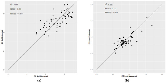
Figure 1.
Best (a) soil and (b) leaf prediction models.
4. Discussion
Soil and leaf EC estimation models were established in this study based on the use of twenty-five machine learning algorithms. It was found that the Gaussian Process Regression models (Sparse Spectrum and Gaussian Processes) met the accuracy requirements and can be used for the quantitative estimation of the soil and leaf EC.
The response of vegetation spectral indices to soil EC is generally affected by many factors, including vegetation cover, salt tolerance, soil moisture, and soil type [75]. The results varied markedly, especially for leaf EC estimation, with better performance obtained from “vegetation indices” [76]. Indeed, in many previous studies, using salinity indices (salinity indices 1, 2, and 3) and vegetation indices (normalized difference infrared index, green normalized difference vegetation index, and a simple ratio) to estimate ECSoil [77,78], the regions with vegetation coverage were directly identified as not salinized regions or slightly salinized regions [16,24,79]. As confirmed by [3], spectral indices are indispensable estimators for soil salinization monitoring. The relationship between spectral indices and electrical conductivity variables is established through fitting functions. However, the use of spectral indices is restricted to formulations that use only a few bands, with at most three or four bands, which implies a decrease in the complete-spectrum dataset [80]. Nowadays, this limits the strength of the estimation methods, as tens or hundreds of spectral bands are available, respectively, in current superspectral [81] or spaceborne hyperspectral sensors [82,83].
Soils with different salinity have different spectral characteristics, which is the basis of the remote sensing monitoring of soil salinization. The key to successfully estimating the soil and leaf salt content using spectral variables is to choose an effective model. Non-parametric regression algorithms (also referred to as machine learning regression algorithms—MLRAs) are data-driven approaches based on the definition of regression functions between the spectral information and the variables of interest. Machine learning algorithms are able to learn autonomously and can solve the problem of complex nonlinear function approximation in estimation of soil and leaf electrical conductivity. The main use of these algorithms in this research is related to the possibility of training them with complete spectral information from the Sentinel-2 multispectral satellite. These adaptive algorithms can cope with the strong non-linearity inherent in remote sensing data [84,85]. As confirmed by [86,87], ML algorithms such as random forest (RF) [88] were demonstrated to be more robust to noisy features, small training sizes, and high dimensionality and collinearity. Indeed, in this case study, because the soil electrical conductivity dataset contains in situ sampling and the corresponding spectral characteristics, non-parametric regression models were applied. The methodology allows electrical conductivity prediction models adjusted to the input variables information and existing observations to be achieved.
As presented in the results (Section 3.3), the Gaussian Process Regression (GPR) models presented the best results and attained a higher performance and accuracy when estimating the electrical conductivity variables (ECSoil: RMSE = 0.132 and R = 0.790; ECLeaf: RMSE = 0.720 and R = 0.716). Indeed, GPR models are efficient machine learning regression algorithms for retrieving biophysical parameters [73]. GPR is based on a Bayesian approach for building generic regression models between the input (remote sensing data) and output (biophysical parameter) variables [81]. Gaussian Process Regression models are nonparametric as well as non-linear, while at the same time providing a ranking of relevant bands (features) from input spectral data obtained from remote sensing tools [89]. Gaussian Process Regression models are flexible enough to fit many types of data, including geospatial and time-series data. In the inference stage, every time a new observation is made, the model hypothesis (prior probability distribution) is updated considering the new observations [90]. For this reason, GPR was evaluated as top-performing in accurately reconstructing time-series datasets [91,92]. Our results agree with the findings of a previous study [26], revealing that GPR is a powerful tool that could be used for soil salinity mapping.
Moreover, both boosting and random forest algorithms presented close statistic results in the range of 0.7 and 0.6 for RMSE and R, respectively, when estimating ECSoil and at the range of 0.2 and 0.6 for RMSE and R, respectively, when predicting ECLeaf. From this perspective, some authors believed that the Gradient Boosting (GB) model added regularization terms, which were beneficial in reducing model complexity, avoiding the overfitting phenomenon, and increasing the generalization ability of the model [93]. In addition, GB supports the parallel splitting process, which improves the efficiency of model construction, optimizes the objective function, and ensures prediction accuracy [94]. As one of boosting algorithms, the GB model places more weight on more important factors in the training–testing process [95]. Therefore, this model shows a minimal reduction in model accuracy. Many studies concluded that the accuracy of the predictions of boosting algorithms depended mainly on the relevance of input parameters [96,97,98]. Our results agree with the findings of [2], in which the authors compared three machine learning models (RF, SVM, and GB) to predict soil salinity parameters. These authors found that GB and RF models showed good prediction ability for some salinity parameters, with a slightly higher performance of the GB model. The same research also showed that all models underestimated salinity variables for high salinity values, which may result in more challenging predictions in soils with higher potential salinity values However, [99] still recommended GB models for extreme values. Moreover, the authors of [100] found that the boosting model performed best, but the simulation results of the RF model were also acceptable.
On the other hand, the accuracy of the random forest model was high. Generally, decision-tree-based algorithms (e.g., RF) require no assumptions about the data distribution, adapt to outliers by isolating them in small regions of the feature space [101], have no hidden layers in their structure, and use tree algorithms for estimation on the basis of pattern recognition [102]. Our finding confirmed previous studies that indicated superior estimation capacity of tree-based models [103,104]. Indeed, due to the nonlinear nature of many environmental phenomena, more flexible models with non-linear structures will yield better results [105].
From this perspective, among the tested machine learning algorithms, the results revealed that RF performed better than support vector regression (SVR), with higher accuracy and a lower root-mean-square error. Our results agree with those of [106]. Indeed, in their research, [106] combined a dataset consisting of Landsat 5 Thematic Mapper and ALOS L-band radar data acquired at the same time as field-measured salinity and used the support vector regression and random forest algorithms for salinity prediction. The results revealed that RF performed better than SVR. The SVR model showed low performance in learning with values of EC greater than 7 mS/cm [26]. These samples caused the low degree-of-fit of the model, and consequently, the model lacked the sensitivity required to predict values with high EC.
Generally, decision-tree-based algorithms (e.g., RF) perform better, particularly in comparison to data-intelligence algorithms with hidden layers in their structures [102]. Hence, GPR, GB, and RF are recommended for soil salinity estimation and mapping.
Recently, the increasing accessibility of the new generation of hyperspectral satellite sensors and the operational enhancements in the retrieval methods are forging the opportunity to attain up-to-date knowledge about the variability in salinity characteristics throughout the Earth system. With the upcoming stream of imaging spectroscopy data with the new, already-launched PRISMA and EnMAP hyperspectral satellites, there is a rising need to differentiate between methodologies, tools, and software applications exploiting the spectral possibilities to extract relevant information on an operational basis to quantify electrical conductivity variables. The quantitative estimation of soil traits considerably relies on the retrieval approach. Moreover, according to the literature, hybrid algorithms, in most cases, are more flexible and can enhance the prediction power of standalone models [107,108,109,110].
5. Conclusions
The results of this research provide a further contribution to the ability of Sentinel-2 spectral data to predict soil and leaf electrical conductivity in an agricultural area in central Tunisia. The performance of twenty-five regression algorithms for estimating electrical conductivity at the soil and vegetation levels was compared and quantitively assessed. Our results indicate that the combined use of machine learning algorithms and Sentinel-2 whole multispectral band set improved the accuracy of the electrical conductivity estimation.
An additional key goal of this research was to investigate the potential of recently developed retrieval regression methodologies for quantifying electrical conductivity not only at the soil level but also at the vegetation (leaf) level.
For future perspectives, the higher spectral resolution of newly launched hyperspectral satellites (e.g., PRISMA and EnMAP) will be a great tool to exploit narrow absorption spectral features in the Vis-NIR and SWIR spectral ranges associated with salinity estimation. Therefore, combining data from hyperspectral sensors with the most advanced machine learning algorithms could represent an innovative and robust strategy for improving the mapping and monitoring of soil and vegetation salinity properties.
Author Contributions
Conceptualization, N.M., O.B., R.A. and A.M.S.; methodology, N.M. and O.B.; software, N.M.; validation, N.M.; formal analysis, N.M.; investigation, N.M. and O.B.; resources, N.M. and O.B.; data curation N.M.; writing—original draft preparation, N.M.; writing—review and editing, N.M., R.A., A.M.S. and M.T.; visualization, N.M., R.A. and A.M.S.; supervision, O.B., M.B. and M.T.; project administration, N.M. and O.B. All authors have read and agreed to the published version of the manuscript.
Funding
This research received no external funding.
Data Availability Statement
Not applicable.
Conflicts of Interest
The authors declare no conflict of interest.
References
- Litalien, A.; Zeeb, B. Curing the Earth: A Review of Anthropogenic Soil Salinization and Plant-Based Strategies for Sustainable Mitigation. Sci. Total Environ. 2020, 698, 134235. [Google Scholar] [CrossRef] [PubMed]
- Xiao, Y.; Zhao, G.; Li, T.; Zhou, X.; Li, J. Soil Salinization of Cultivated Land in Shandong Province, China—Dynamics during the Past 40 Years. Land Degrad Dev. 2019, 30, 426–436. [Google Scholar] [CrossRef]
- Wang, J.; Peng, J.; Li, H.; Yin, C.; Liu, W.; Wang, T.; Zhang, H. Soil Salinity Mapping Using Machine Learning Algorithms with the Sentinel-2 MSI in Arid Areas, China. Remote Sens. 2021, 13, 305. [Google Scholar] [CrossRef]
- Zhang, X.; Huang, B. Prediction of Soil Salinity with Soil-Reflected Spectra: A Comparison of Two Regression Methods. Sci. Rep. 2019, 9, 5067. [Google Scholar] [CrossRef]
- Hafez, E.M.; Omara, A.E.D.; Alhumaydhi, F.A.; El-Esawi, M.A. Minimizing Hazard Impacts of Soil Salinity and Water Stress on Wheat Plants by Soil Application of Vermicompost and Biochar. Physiol. Plant. 2021, 172, 587–602. [Google Scholar] [CrossRef] [PubMed]
- Deng, G.; Yao, X.; Jiang, H.; Cao, Y.; Wen, Y.; Wang, W.; Zhao, S.; He, C. Study on the Ecological Operation and Watershed Management of Urban Rivers in Northern China. Water 2020, 12, 914. [Google Scholar] [CrossRef]
- Ma, L.; Yang, S.; Simayi, Z.; Gu, Q.; Li, J.; Yang, X.; Ding, J. Modeling Variations in Soil Salinity in the Oasis of Junggar Basin, China. Land Degrad. Dev. 2018, 29, 551–562. [Google Scholar] [CrossRef]
- Vermeulen, D.; van Niekerk, A. Machine Learning Performance for Predicting Soil Salinity Using Different Combinations of Geomorphometric Covariates. Geoderma 2017, 299, 1–12. [Google Scholar] [CrossRef]
- Zhang, Y.; Biswas, A.; Adamchuk, V.I. Implementation of a Sigmoid Depth Function to Describe Change of Soil PH with Depth. Geoderma 2017, 289, 1–10. [Google Scholar] [CrossRef]
- Shoshany, M.; Goldshleger, N.; Chudnovsky, A. Monitoring of Agricultural Soil Degradation by Remote-Sensing Methods: A Review. Int. J. Remote. Sens. 2013, 34, 6152–6181. [Google Scholar] [CrossRef]
- Xiao, C.; Ji, Q.; Chen, J.; Zhang, F.; Li, Y.; Fan, J.; Hou, X.; Yan, F.; Wang, H. Prediction of Soil Salinity Parameters Using Machine Learning Models in an Arid Region of Northwest China. Comput. Electron. Agric. 2023, 204, 107512. [Google Scholar] [CrossRef]
- Hossain, M.S.; Rahman, G.K.M.M.; Solaiman, A.R.M.; Alam, M.S.; Rahman, M.M.; Mia, M.A.B. Estimating Electrical Conductivity for Soil Salinity Monitoring Using Various Soil-Water Ratios Depending on Soil Texture. Commun. Soil Sci. Plant Anal. 2020, 51, 635–644. [Google Scholar] [CrossRef]
- Corwin, D.L.; Yemoto, K. Salinity: Electrical Conductivity and Total Dissolved Solids. Methods Soil Anal. 2017, 2, 1442–1461. [Google Scholar] [CrossRef]
- Corwin, D.L.; Lesch, S.M. Characterizing Soil Spatial Variability with Apparent Soil Electrical Conductivity: I. Survey Protocols. Comput. Electron. Agric. 2005, 46, 103–133. [Google Scholar] [CrossRef]
- Chabrillat, S.; Ben-Dor, E.; Cierniewski, J.; Gomez, C.; Schmid, T.; van Wesemael, B. Imaging Spectroscopy for Soil Mapping and Monitoring. Surv. Geophys. 2019, 40, 361–399. [Google Scholar] [CrossRef]
- Ward, K.J.; Chabrillat, S.; Brell, M.; Castaldi, F.; Spengler, D.; Foerster, S. Mapping Soil Organic Carbon for Airborne and Simulated Enmap Imagery Using the Lucas Soil Database and a Local Plsr. Remote Sens. 2020, 12, 3451. [Google Scholar] [CrossRef]
- Omran, E.S.E. Rapid Prediction of Soil Mineralogy Using Imaging Spectroscopy. Eur. Soil Sci. 2017, 50, 597–612. [Google Scholar] [CrossRef]
- Zeng, W.; Xu, C.; Huang, J.; Wu, J.; Tuller, M. Predicting Near-Surface Moisture Content of Saline Soils from Near-Infrared Reflectance Spectra with a Modified Gaussian Model. Soil Sci. Soc. Am. J. 2016, 80, 1496–1506. [Google Scholar] [CrossRef]
- Gomez, C.; Oltra-Carrió, R.; Bacha, S.; Lagacherie, P.; Briottet, X. Evaluating the Sensitivity of Clay Content Prediction to Atmospheric Effects and Degradation of Image Spatial Resolution Using Hyperspectral VNIR/SWIR Imagery. Remote Sens. Environ. 2015, 164, 1–15. [Google Scholar] [CrossRef]
- Sadeghi, M.; Babaeian, E.; Tuller, M.; Jones, S.B. Particle Size Effects on Soil Reflectance Explained by an Analytical Radiative Transfer Model. Remote Sens. Environ. 2018, 210, 375–386. [Google Scholar] [CrossRef]
- Yuan, J.; Wang, X.; Yan, C.; Chen, S.; Wang, S.; Zhang, J.; Xu, Z.; Ju, X.; Ding, N.; Dong, Y.; et al. Wavelength Selection for Estimating Soil Organic Matter Contents through the Radiative Transfer Model. IEEE Access 2020, 8, 176286–176293. [Google Scholar] [CrossRef]
- Sidike, A.; Zhao, S.; Wen, Y. Estimating Soil Salinity in Pingluo County of China Using QuickBird Data and Soil Reflectance Spectra. Int. J. Appl. Earth Obs. Geoinf. 2014, 26, 156–175. [Google Scholar] [CrossRef]
- Nawar, S.; Buddenbaum, H.; Hill, J. Estimation of Soil Salinity Using Three Quantitative Methods Based on Visible and Near-Infrared Reflectance Spectroscopy: A Case Study from Egypt. Arab. J. Geosci. 2015, 8, 5127–5140. [Google Scholar] [CrossRef]
- Ding, J.; Yu, D. Monitoring and Evaluating Spatial Variability of Soil Salinity in Dry and Wet Seasons in the Werigan–Kuqa Oasis, China, Using Remote Sensing and Electromagnetic Induction Instruments. Geoderma 2014, 235–236, 316–322. [Google Scholar] [CrossRef]
- Xu, H.; Chen, C.; Zheng, H.; Luo, G.; Yang, L.; Wang, W.; Wu, S.; Ding, J. AGA-SVR-Based Selection of Feature Subsets and Optimization of Parameter in Regional Soil Salinization Monitoring. Int. J. Remote Sens. 2020, 41, 4470–4495. [Google Scholar] [CrossRef]
- Hoa, P.V.; Giang, N.V.; Binh, N.A.; Hai, L.V.H.; Pham, T.-D.; Hasanlou, M.; Bui, D.T. Soil Salinity Mapping Using SAR Sentinel-1 Data and Advanced Machine Learning Algorithms: A Case Study at Ben Tre Province of the Mekong River Delta (Vietnam). Remote Sens. 2019, 11, 128. [Google Scholar] [CrossRef]
- Mzid, N. Assessment of Remote-Based Vegetation Indices to Face Agriculture Challenges in The Mediterranean. 2021, 1–134. Available online: https://www.interregir2ma.eu/images/IR2MA/deliverables/242_Workshop/P6_IRM2A_Workshop_Mzid.pdf (accessed on 18 September 2020).
- DGACTA. Examen et Évaluation de La Situation Actuelle de La Salinisation Des Sols et Préparation d’un Plan d’action de Lutte Contre Ce Fléau Dans Les Périmètres Irrigués En Tunisie. In Phase 2: Ebauche Du Plan D’action; DGACTA, Ministère de L’agriculture et des Ressources Hydrauliques: Tunisie, Tunisie, 2007. [Google Scholar]
- Hachicha, M. Les Sols Salés et Leur Mise En Valeur En Tunisie. Sécher. Montroug. 2007, 18, 45–50. [Google Scholar] [CrossRef]
- Zarai, B.; Walter, C.; Michot, D.; Montoroi, J.P.; Hachicha, M. Integrating Multiple Electromagnetic Data to Map Spatiotemporal Variability of Soil Salinity in Kairouan Region, Central Tunisia. J. Arid. Land 2022, 14, 186–202. [Google Scholar] [CrossRef]
- Ibrahimi, K.; Khader, N.; Adouni, L. Soil Salinity Assessment and Characterization in Abandoned Farmlands of Metouia Oasis, South Tunisia. Environ. Sci. Proc. 2022, 16, 3. [Google Scholar] [CrossRef]
- Todorovic, M. An Excel-Based Tool for Real-Time Irrigation Management At Field Scale. In Proceedings of the International Symposium on Water and Land Management for Sustainable Irrigated Agriculture, Dublin, Ireland, 31 January 1992; pp. 1–11. [Google Scholar]
- Allen, R.G.; Pereira, L.S.; Raes, D. Crop Evapotranspiration (Guidelines for Computing Crop Water Requirements); FAO: Rome, Italy; Available online: https://appgeodb.nancy.inra.fr/biljou/pdf/Allen_FAO1998.pdf (accessed on 17 September 2020).
- Ayers, R.S.; Westcot, D.W. Water Quality for Agriculture; FAO: Rome, Italy, 1985. Available online: https://www.waterboards.ca.gov/water_issues/programs/tmdl/records/state_board/1985/ref2648.pdf (accessed on 18 September 2020).
- Ismail, O.M. Use of Electrical Conductivity as a Tool for Determining Damage Index of Some Mango Cultivars. Int. J. Plant Soil Sci. 2014, 3, 448–456. [Google Scholar] [CrossRef]
- Khan, N.M.; Rastoskuev, V.V.; Sato, Y.; Shiozawa, S. Assessment of Hydrosaline Land Degradation by Using a Simple Approach of Remote Sensing Indicators. Agric. Water Manag. 2005, 77, 96–109. [Google Scholar] [CrossRef]
- Abbas, M.A.; Khan, S. Using Remote Sensing Techniques for Appraisal of Irrigated Soil Salinity. In Proceedings of the International Congress on Modelling and Simulation (MODSIM), Christchurch, New Zealand, December 2007; Modelling and Simulation Society of Australia and New Zealand: Brighton, UK, 2007; pp. 2632–2638. [Google Scholar]
- Daughtry, C.S.T.; Walthall, C.L.; Kim, M.S.; de Colstoun, E.B.; McMurtrey, J.E. Estimating Corn Leaf Chlorophyll Concentration from Leaf and Canopy Reflectance. Remote Sens. Environ. 2000, 74, 229–239. [Google Scholar] [CrossRef]
- Rouse, J.W., Jr.; Haas, R.H.; Schell, J.A.; Deering, D.W.; Rouse, J.W., Jr.; Haas, R.H.; Schell, J.A.; Deering, D.W. Monitoring Vegetation Systems in the Great Plains with Erts. NASSP 1974, 351, 309. [Google Scholar]
- Huete, A.R. A Soil-Adjusted Vegetation Index (SAVI). Remote Sens. Environ. 1988, 25, 295–309. [Google Scholar] [CrossRef]
- Huete, A.; Didan, K.; Miura, T.; Rodriguez, E.P.; Gao, X.; Ferreira, L.G. Overview of the Radiometric and Biophysical Performance of the MODIS Vegetation Indices. Remote Sens. Environ. 2002, 83, 195–213. [Google Scholar] [CrossRef]
- Saleska, S.R.; Didan, K.; Huete, A.R.; da Rocha, H.R. Amazon Forests Green-up during 2005 Drought. Science 2007, 318, 612. [Google Scholar] [CrossRef]
- Wu, W. The Generalized Difference Vegetation Index (GDVI) for Dryland Characterization. Remote Sens. 2014, 6, 1211–1233. [Google Scholar] [CrossRef]
- Wang, L.; Qu, J.J. NMDI: A Normalized Multi-Band Drought Index for Monitoring Soil and Vegetation Moisture with Satellite Remote Sensing. Geophys. Res. Lett. 2007, 34. [Google Scholar] [CrossRef]
- Fensholt, R.; Sandholt, I. Derivation of a Shortwave Infrared Water Stress Index from MODIS Near- and Shortwave Infrared Data in a Semiarid Environment. Remote Sens. Environ. 2003, 87, 111–121. [Google Scholar] [CrossRef]
- Ceccato, P.; Flasse, S.; Tarantola, S.; Jacquemoud, S.; Grégoire, J.-M. Detecting Vegetation Leaf Water Content Using Reflectance in the Optical Domain. Remote Sens. Environ. 2001, 77, 22–33. [Google Scholar] [CrossRef]
- Hunt, E.R.; Rock, B.N. Detection of Changes in Leaf Water Content Using Near- and Middle-Infrared Reflectances. Remote Sens. Environ. 1989, 30, 43–54. [Google Scholar] [CrossRef]
- Haboudane, D.; Miller, J.R.; Tremblay, N.; Zarco-Tejada, P.J.; Dextraze, L. Integrated Narrow-Band Vegetation Indices for Prediction of Crop Chlorophyll Content for Application to Precision Agriculture. Remote Sens. Environ. 2002, 81, 416–426. [Google Scholar] [CrossRef]
- Vincini, M.; Frazzi, E.; D’Alessio, P. A Broad-Band Leaf Chlorophyll Vegetation Index at the Canopy Scale. Precis. Agric. 2008, 9, 303–319. [Google Scholar] [CrossRef]
- Hernandez-Clemente, R.; Navarro-Cerrillo, R.M.; Zarco-Tejada, P.J. Deriving Predictive Relationships of Carotenoid Content at the Canopy Level in a Conifer Forest Using Hyperspectral Imagery and Model Simulation. IEEE Trans. Geosci. Remote Sens. 2014, 52, 5206–5217. [Google Scholar] [CrossRef]
- IDB—Index: TCARI/OSAVI. Available online: https://www.indexdatabase.de/db/i-single.php?id=191 (accessed on 29 January 2023).
- Clevers, J.G.P.W.; Kooistra, L.; van den Brande, M.M.M. Using Sentinel-2 Data for Retrieving LAI and Leaf and Canopy Chlorophyll Content of a Potato Crop. Remote Sens. 2017, 9, 405. [Google Scholar] [CrossRef]
- Kamenova, I.; Dimitrov, P. Evaluation of Sentinel-2 Vegetation Indices for Prediction of LAI, FAPAR and FCover of Winter Wheat in Bulgaria. Eur. J. Remote. Sens. 2020, 54, 89–108. [Google Scholar] [CrossRef]
- Zarco-Tejada, P.J.; Hornero, A.; Beck, P.S.A.; Kattenborn, T.; Kempeneers, P.; Hernández-Clemente, R. Chlorophyll Content Estimation in an Open-Canopy Conifer Forest with Sentinel-2A and Hyperspectral Imagery in the Context of Forest Decline. Remote Sens. Environ. 2019, 223, 320–335. [Google Scholar] [CrossRef]
- Huang, Y.; Qiu, B.; Chen, C.; Zhu, X.; Wu, W.; Jiang, F.; Lin, D.; Peng, Y. Automated Soybean Mapping Based on Canopy Water Content and Chlorophyll Content Using Sentinel-2 Images. Int. J. Appl. Earth Obs. Geoinf. 2022, 109, 102801. [Google Scholar] [CrossRef]
- IDB—Index: Modified Chlorophyll Absorption in Reflectance Index. Available online: https://www.indexdatabase.de/db/i-single.php?id=41 (accessed on 29 January 2023).
- Maleki, M.; Arriga, N.; Barrios, J.M.; Wieneke, S.; Liu, Q.; Peñuelas, J.; Janssens, I.A.; Balzarolo, M. Estimation of Gross Primary Productivity (GPP) Phenology of a Short-Rotation Plantation Using Remotely Sensed Indices Derived from Sentinel-2 Images. Remote Sens. 2020, 12, 2104. [Google Scholar] [CrossRef]
- Frampton, W.J.; Dash, J.; Watmough, G.; Milton, E.J. Evaluating the Capabilities of Sentinel-2 for Quantitative Estimation of Biophysical Variables in Vegetation. ISPRS J. Photogramm. Remote Sens. 2013, 82, 83–92. [Google Scholar] [CrossRef]
- Nguyen, N.; Binh, N.; Nguyen, B. Potential of Drought Monitoring Using Sentinel-2 Data; GIS-IDEAS. 2016. Available online: https://www.humg.edu.vn (accessed on 18 January 2021).
- Wang, L.; Qu, J.J.; Hao, X. Forest Fire Detection Using the Normalized Multi-Band Drought Index (NMDI) with Satellite Measurements. Agric. For. Meteorol. 2008, 148, 1767–1776. [Google Scholar] [CrossRef]
- Liu, Y.; Qian, J.; Yue, H. Combined Sentinel-1A with Sentinel-2A to Estimate Soil Moisture in Farmland. IEEE J. Sel. Top. Appl. Earth Obs. Remote Sens. 2021, 14, 1292–1310. [Google Scholar] [CrossRef]
- Markov, B. Comparison of Remote Sensing-Based Indexes for Monitoring Drought Impact on Forest Ecosystems. In Annual of Sofia University “St. Kliment Ohridski” Faculty of Geology and Geography Book 2; 2018; Volume 11, pp. 237–246. [Google Scholar]
- Chen, Y.; Qiu, Y.; Zhang, Z.; Zhang, J.; Chen, C.; Han, J.; Liu, D. Estimating Salt Content of Vegetated Soil at Different Depths with Sentinel-2 Data. PeerJ 2020, 8, e10585. [Google Scholar] [CrossRef]
- Meyer, L.H.; Heurich, M.; Beudert, B.; Premier, J.; Pflugmacher, D. Comparison of Landsat-8 and Sentinel-2 Data for Estimation of Leaf Area Index in Temperate Forests. Remote Sens. 2019, 11, 1160. [Google Scholar] [CrossRef]
- Hamrouni, Y.; Paillassa, E.; Chéret, V.; Monteil, C.; Sheeren, D. Sentinel-2 Poplar Index for Operational Mapping of Poplar Plantations over Large Areas. Remote Sens. 2022, 14, 3975. [Google Scholar] [CrossRef]
- Sonobe, R.; Yamaya, Y.; Tani, H.; Wang, X.; Kobayashi, N.; Mochizuki, K.-I. Crop Classification from Sentinel-2-Derived Vegetation Indices Using Ensemble Learning. J. Appl. Remote Sens. 2018, 12, 026019. [Google Scholar] [CrossRef]
- Kobayashi, N.; Tani, H.; Wang, X.; Sonobe, R. Crop Classification Using Spectral Indices Derived from Sentinel-2A Imagery. J. Inf. Telecommun. 2019, 4, 67–90. [Google Scholar] [CrossRef]
- IDB—Index: Normalized Difference 860/1640. Available online: https://www.indexdatabase.de/db/i-single.php?id=219 (accessed on 29 January 2023).
- Elhag, M.; Bahrawi, J.A. Soil Salinity Mapping and Hydrological Drought Indices Assessment in Arid Environments Based on Remote Sensing Techniques. Geosci. Instrum. Methods Data Syst. 2017, 6, 149–158. [Google Scholar] [CrossRef]
- IDB—Index: Simple Ratio 1600/820 Moisture Stress Index. Available online: https://www.indexdatabase.de/db/i-single.php?id=48 (accessed on 29 January 2023).
- Verrelst, J.; Romijn, E.; Kooistra, L. Mapping Vegetation Density in a Heterogeneous River Floodplain Ecosystem Using Pointable CHRIS/PROBA Data. Remote Sens. 2012, 4, 2866–2889. [Google Scholar] [CrossRef]
- Rivera, J.P.; Verrelst, J.; Delegido, J.; Veroustraete, F.; Moreno, J. On the Semi-Automatic Retrieval of Biophysical Parameters Based on Spectral Index Optimization. Remote Sens. 2014, 6, 4927–4951. [Google Scholar] [CrossRef]
- Pablo, J.; Caicedo, R.; Verrelst, J.; Muñoz-Marí, J.; Moreno, J.; Camps-Valls, G. Toward a Semiautomatic Machine Learning Retrieval of Biophysical Parameters. IEEE J. Sel. Top. Appl. Earth Obs. Remote Sens. 2014, 7, 1249–1259. [Google Scholar] [CrossRef]
- Rivera, J.P.; Verrelst, J.; Leonenko, G.; Moreno, J. Multiple Cost Functions and Regularization Options for Improved Retrieval of Leaf Chlorophyll Content and LAI through Inversion of the PROSAIL Model. Remote Sens. 2013, 5, 3280–3304. [Google Scholar] [CrossRef]
- Metternicht, G.I.; Zinck, J.A. Remote Sensing of Soil Salinity: Potentials and Constraints. Remote Sens. Environ. 2003, 85, 1–20. [Google Scholar] [CrossRef]
- Allbed, A.; Kumar, L.; Aldakheel, Y.Y. Assessing Soil Salinity Using Soil Salinity and Vegetation Indices Derived from IKONOS High-Spatial Resolution Imageries: Applications in a Date Palm Dominated Region. Geoderma 2014, 230–231, 1–8. [Google Scholar] [CrossRef]
- Celleri, C.; Zapperi, G.; Trilla, G.G.; Pratolongo, P. Assessing the Capability of Broadband Indices Derived from Landsat 8 Operational Land Imager to Monitor above Ground Biomass and Salinity in Semiarid Saline Environments of the Bahía Blanca Estuary, Argentina. Int. J. Remote Sens. 2019, 40, 4817–4838. [Google Scholar] [CrossRef]
- Allbed, A.; Kumar, L. Soil Salinity Mapping and Monitoring in Arid and Semi-Arid Regions Using Remote Sensing Technology: A Review. Adv. Remote. Sens. 2013, 2, 373–385. [Google Scholar] [CrossRef]
- Pakparvar, M.; Gabriels, D.; Aarabi, K.; Edraki, M.; Raes, D.; Cornelis, W. Incorporating Legacy Soil Data to Minimize Errors in Salinity Change Detection: A Case Study of Darab Plain, Iran. Int. J. Remote Sens. 2012, 33, 6215–6238. [Google Scholar] [CrossRef]
- Verrelst, J.; Malenovský, Z.; van der Tol, C.; Camps-Valls, G.; Gastellu-Etchegorry, J.-P.; Lewis, P.; North, P.; Moreno, J. Quantifying Vegetation Biophysical Variables from Imaging Spectroscopy Data: A Review on Retrieval Methods. Surv. Geophys. 2019, 40, 589–629. [Google Scholar] [CrossRef]
- Verrelst, J.; Camps-Valls, G.; Muñoz-Marí, J.; Rivera, J.P.; Veroustraete, F.; Clevers, J.G.P.W.; Moreno, J. Optical Remote Sensing and the Retrieval of Terrestrial Vegetation Bio-Geophysical Properties—A Review. ISPRS J. Photogramm. Remote Sens. 2015, 108, 273–290. [Google Scholar] [CrossRef]
- Pignatti, S.; Acito, N.; Amato, U.; Casa, R.; Castaldi, F.; Coluzzi, R.; de Bonis, R.; Diani, M.; Imbrenda, V.; Laneve, G.; et al. Environmental Products Overview of the Italian Hyperspectral Prisma Mission: The SAP4PRISMA Project. In Proceedings of the 2015 IEEE International Geoscience and Remote Sensing Symposium (IGARSS), Milan, Italy, 26–31 July 2015; Institute of Electrical and Electronics Engineers Inc.: Piscataway, NJ, USA; pp. 3997–4000. [Google Scholar]
- Guanter, L.; Kaufmann, H.; Segl, K.; Foerster, S.; Rogass, C.; Chabrillat, S.; Kuester, T.; Hollstein, A.; Rossner, G.; Chlebek, C.; et al. The EnMAP Spaceborne Imaging Spectroscopy Mission for Earth Observation. Remote Sens. 2015, 7, 8830–8857. [Google Scholar] [CrossRef]
- Verrelst, J.; Muñoz, J.; Alonso, L.; Delegido, J.; Rivera, J.P.; Camps-Valls, G.; Moreno, J. Machine Learning Regression Algorithms for Biophysical Parameter Retrieval: Opportunities for Sentinel-2 and -3. Remote Sens. Environ. 2012, 118, 127–139. [Google Scholar] [CrossRef]
- Knudby, A.; LeDrew, E.; Brenning, A. Predictive Mapping of Reef Fish Species Richness, Diversity and Biomass in Zanzibar Using IKONOS Imagery and Machine-Learning Techniques. Remote Sens. Environ. 2010, 114, 1230–1241. [Google Scholar] [CrossRef]
- Jiapaer, G.; Liang, S.; Yi, Q.; Liu, J. Vegetation Dynamics and Responses to Recent Climate Change in Xinjiang Using Leaf Area Index as an Indicator. Ecol. Indic. 2015, 58, 64–76. [Google Scholar] [CrossRef]
- Houborg, R.; McCabe, M.F. Daily Retrieval of NDVI and LAI at 3 m Resolution via the Fusion of CubeSat, Landsat, and MODIS Data. Remote Sens. 2018, 10, 890. [Google Scholar] [CrossRef]
- Breiman, L. Random Forests. Mach. Learn. 2001, 45, 5–32. [Google Scholar] [CrossRef]
- Aghababaei, M.; Ebrahimi, A.; Naghipour, A.A.; Asadi, E.; Pérez-Suay, A.; Morata, M.; Garcia, J.L.; Caicedo, J.P.R.; Verrelst, J. Introducing ARTMO’s Machine-Learning Classification Algorithms Toolbox: Application to Plant-Type Detection in a Semi-Steppe Iranian Landscape. Remote Sens. 2022, 14, 4452. [Google Scholar] [CrossRef]
- Caballero, G.; Pezzola, A.; Winschel, C.; Casella, A.; Angonova, P.S.; Rivera-Caicedo, J.P.; Berger, K.; Verrelst, J.; Delegido, J. Seasonal Mapping of Irrigated Winter Wheat Traits in Argentina with a Hybrid Retrieval Workflow Using Sentinel-2 Imagery. Remote Sens. 2022, 14, 4531. [Google Scholar] [CrossRef] [PubMed]
- Belda, S.; Pipia, L.; Morcillo-Pallarés, P.; Rivera-Caicedo, J.P.; Amin, E.; de Grave, C.; Verrelst, J. DATimeS: A Machine Learning Time Series GUI Toolbox for Gap-Filling and Vegetation Phenology Trends Detection. Environ. Model. Softw. 2020, 127, 104666. [Google Scholar] [CrossRef]
- Pipia, L.; Muñoz-Marí, J.; Amin, E.; Belda, S.; Camps-Valls, G.; Verrelst, J. Fusing Optical and SAR Time Series for LAI Gap Filling with Multioutput Gaussian Processes. Remote Sens. Environ. 2019, 235, 111452. [Google Scholar] [CrossRef] [PubMed]
- Nguyen-Sy, T.; To, Q.-D.; Vu, M.-N.; Nguyen, T.-D.; Nguyen, T.-T. Predicting the Electrical Conductivity of Brine-Saturated Rocks Using Machine Learning Methods. J. Appl. Geophys. 2021, 184, 104238. [Google Scholar] [CrossRef]
- Feng, Y.; Liu, L.; Shu, J. A Link Quality Prediction Method for Wireless Sensor Networks Based on Xgboost. IEEE Access 2019, 7, 155229–155241. [Google Scholar] [CrossRef]
- Yan, S.; Wu, L.; Fan, J.; Zhang, F.; Zou, Y.; Wu, Y. A Novel Hybrid WOA-XGB Model for Estimating Daily Reference Evapotranspiration Using Local and External Meteorological Data: Applications in Arid and Humid Regions of China. Agric. Water Manag. 2021, 244, 106594. [Google Scholar] [CrossRef]
- Liu, P.; Wang, J.; Sangaiah, A.K.; Xie, Y.; Yin, X. Analysis and Prediction of Water Quality Using LSTM Deep Neural Networks in IoT Environment. Sustainability 2019, 11, 2058. [Google Scholar] [CrossRef]
- Chen, K.; Chen, H.; Zhou, C.; Huang, Y.; Qi, X.; Shen, R.; Liu, F.; Zuo, M.; Zou, X.; Wang, J.; et al. Comparative Analysis of Surface Water Quality Prediction Performance and Identification of Key Water Parameters Using Different Machine Learning Models Based on Big Data. Water Res. 2020, 171, 115454. [Google Scholar] [CrossRef]
- Yaseen, Z.M. An Insight into Machine Learning Models Era in Simulating Soil, Water Bodies and Adsorption Heavy Metals: Review, Challenges and Solutions. Chemosphere 2021, 277, 130126. [Google Scholar] [CrossRef]
- Gharaibeh, M.A.; Albalasmeh, A.A.; Pratt, C.; el Hanandeh, A. Estimation of Exchangeable Sodium Percentage from Sodium Adsorption Ratio of Salt-Affected Soils Using Traditional and Dilution Extracts, Saturation Percentage, Electrical Conductivity, and Generalized Regression Neural Networks. Catena 2021, 205, 105466. [Google Scholar] [CrossRef]
- el Bilali, A.; Taleb, A.; Brouziyne, Y. Groundwater Quality Forecasting Using Machine Learning Algorithms for Irrigation Purposes. Agric. Water Manag. 2021, 245, 106625. [Google Scholar] [CrossRef]
- Loh, W.-Y. Classification and Regression Trees. WIREs Data Min. Knowl. Discov. 2011, 1, 14–23. [Google Scholar] [CrossRef]
- Kisi, O.; Dailr, A.H.; Cimen, M.; Shiri, J. Suspended Sediment Modeling Using Genetic Programming and Soft Computing Techniques. J. Hydrol. 2012, 450–451, 48–58. [Google Scholar] [CrossRef]
- Choubin, B.; Darabi, H.; Rahmati, O.; Sajedi-Hosseini, F.; Kløve, B. River Suspended Sediment Modelling Using the CART Model: A Comparative Study of Machine Learning Techniques. Sci. Total Environ. 2018, 615, 272–281. [Google Scholar] [CrossRef]
- Melesse, A.M.; Khosravi, K.; Tiefenbacher, J.P.; Heddam, S.; Kim, S.; Mosavi, A.; Pham, B.T. River Water Salinity Prediction Using Hybrid Machine Learning Models. Water 2020, 12, 2951. [Google Scholar] [CrossRef]
- Johns, K.A.; Emslie, M.J.; Hoey, A.S.; Osborne, K.; Jonker, M.J.; Cheal, A.J. Macroalgal Feedbacks and Substrate Properties Maintain a Coral Reef Regime Shift. Ecosphere 2018, 9, e02349. [Google Scholar] [CrossRef]
- Wu, W.; Zucca, C.; Muhaimeed, A.S.; Al-Shafie, W.M.; Al-Quraishi, A.M.F.; Nangia, V.; Zhu, M.; Liu, G. Soil Salinity Prediction and Mapping by Machine Learning Regression in Central Mesopotamia, Iraq. Land Degrad. Dev. 2018, 29, 4005–4014. [Google Scholar] [CrossRef]
- Ghorbani, M.A.; Aalami, M.T.; Naghipour, L. Use of Artificial Neural Networks for Electrical Conductivity Modeling in Asi River. Appl. Water Sci. 2017, 7, 1761–1772. [Google Scholar] [CrossRef]
- Khozani, Z.S.; Khosravi, K.; Pham, B.T.; Kløve, B.; Mohtar, W.H.M.W.; Yaseen, Z.M. Determination of Compound Channel Apparent Shear Stress: Application of Novel Data Mining Models. J. Hydroinfor. 2019, 21, 798–811. [Google Scholar] [CrossRef]
- Pham, B.T.; Prakash, I.; Khosravi, K.; Chapi, K.; Trinh, P.T.; Ngo, T.Q.; Hosseini, S.V.; Bui, D.T. A Comparison of Support Vector Machines and Bayesian Algorithms for Landslide Susceptibility Modelling. Geocarto Int. 2018, 34, 1385–1407. [Google Scholar] [CrossRef]
- Khosravi, K.; Mao, L.; Kisi, O.; Yaseen, Z.M.; Shahid, S. Quantifying Hourly Suspended Sediment Load Using Data Mining Models: Case Study of a Glacierized Andean Catchment in Chile. J. Hydrol. 2018, 567, 165–179. [Google Scholar] [CrossRef]

Disclaimer/Publisher’s Note: The statements, opinions and data contained in all publications are solely those of the individual author(s) and contributor(s) and not of MDPI and/or the editor(s). MDPI and/or the editor(s) disclaim responsibility for any injury to people or property resulting from any ideas, methods, instructions or products referred to in the content. |
© 2023 by the authors. Licensee MDPI, Basel, Switzerland. This article is an open access article distributed under the terms and conditions of the Creative Commons Attribution (CC BY) license (https://creativecommons.org/licenses/by/4.0/).