
Soil Salinity Assessing and Mapping Using Several Statistical and Distribution Techniques in Arid and Semi-Arid Ecosystems, Egypt

 ,
, 
 ,
,  , , ,
, , ,  ,
,  and
and 
Abstract
1. Introduction
2. Materials and Methods
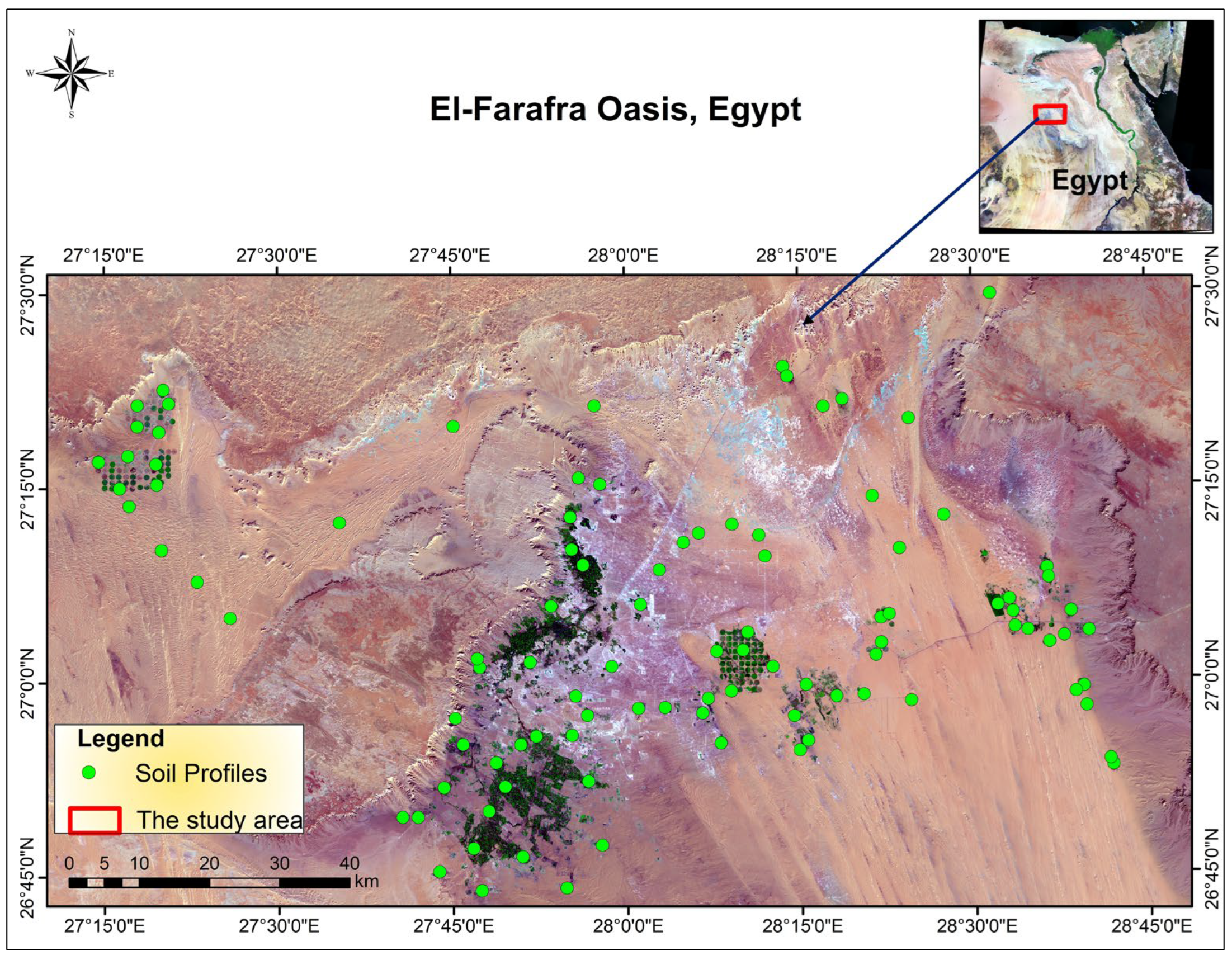
2.1. The Investigated Area
2.2. Remote Sensing and GIS Procedures
- The Landsat-8 (OLI) satellite image data were radiometrically, geometrically, and atmospherically corrected using ENVI 5.1 software [26] to minimize the radiometric distortions and atmospheric perturbations caused by clouds, aerosols, and other atmospheric particles, respectively. These data were downloaded from the United States Geological Survey (USGS) website through Path, 178 and Row, 41 obtained on 8 December 2021.
- Field electrical conductivity (ECe dS m−1) measurements were conducted in May–July 2021. The soil salinity maps were generated using ArcGIS 10.2.2 software [27].
2.3. Field and Laboratory Work
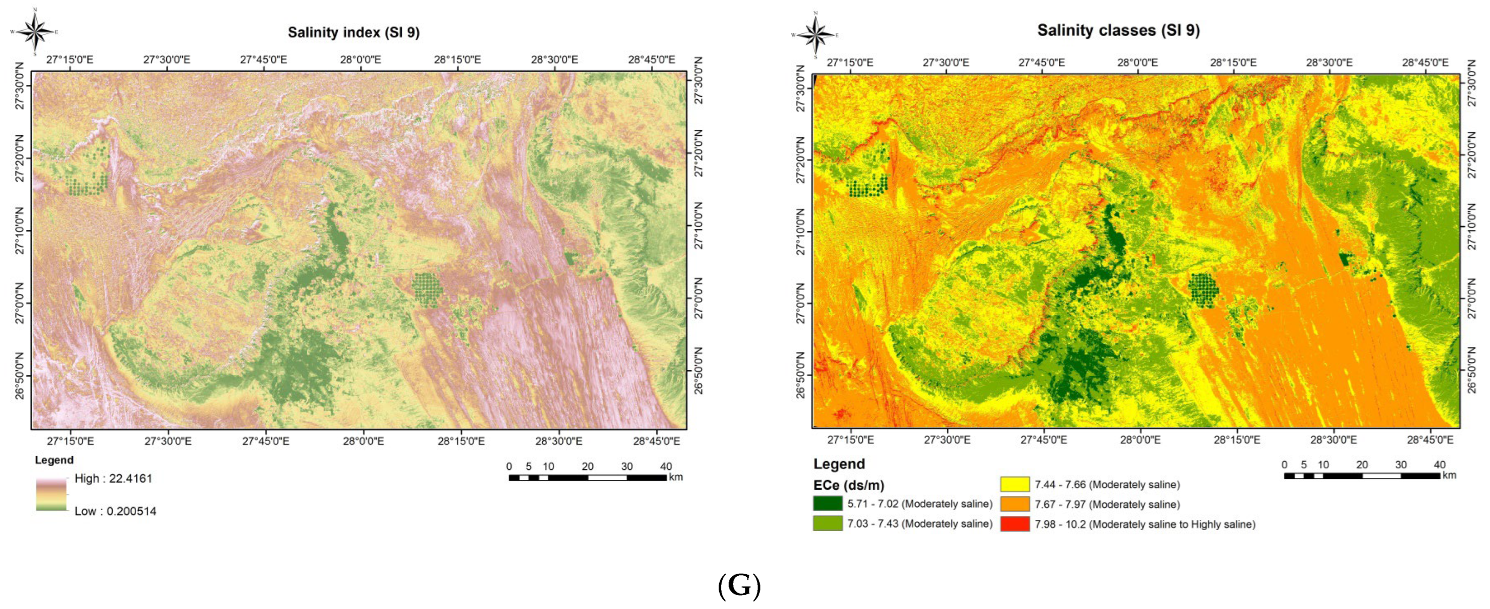
2.4. Soil Salinity Mapping
2.5. Spatial Distribution Mapping (Geostatistical Workflow)
2.6. Developed Linear Regression Model
2.6.1. Pearson Correlation Coefficient Analysis
2.6.2. Root Mean Square Error (RMSE)
2.6.3. Tukey’s Range, Significant and Difference Test (Model Validation)
3. Results
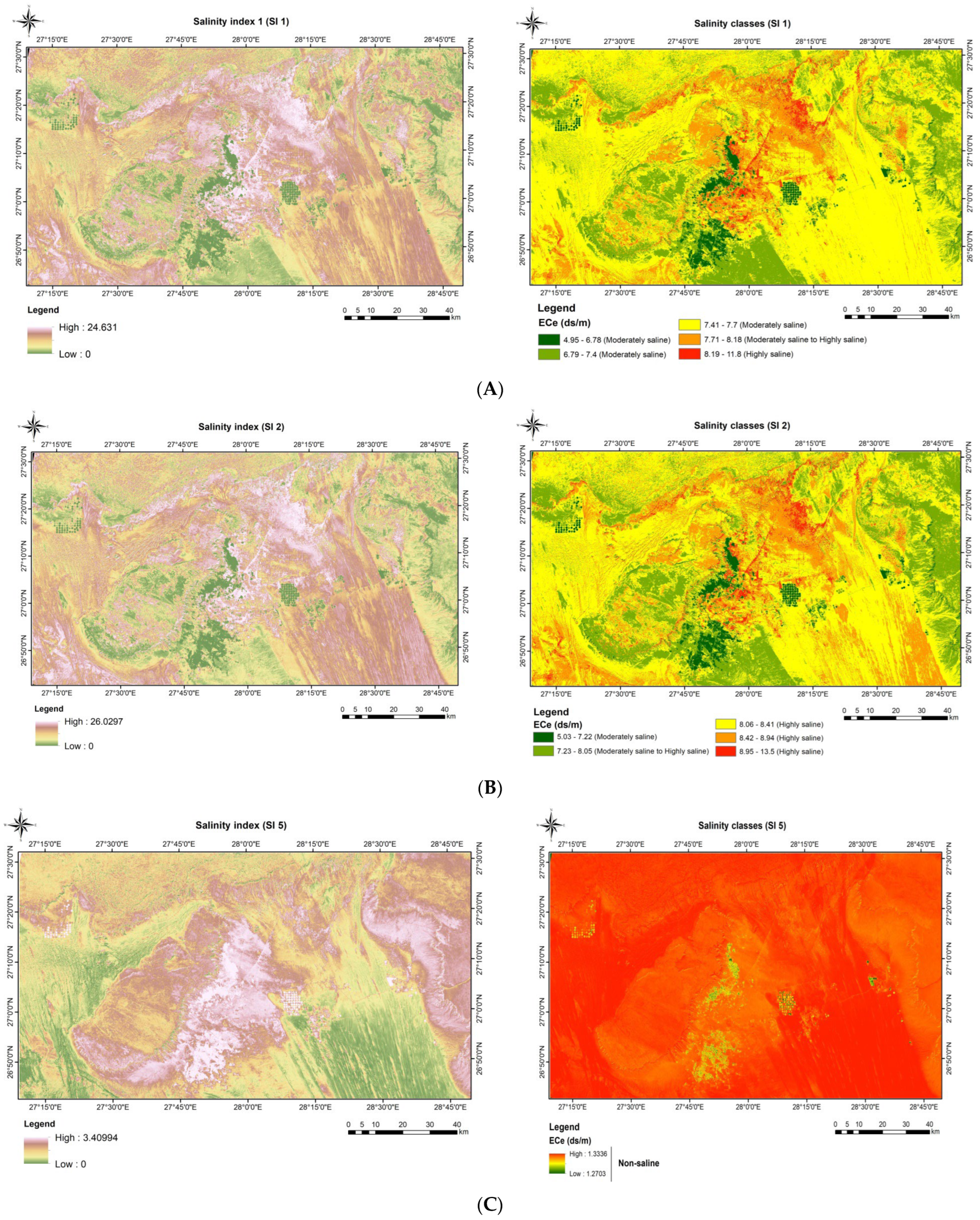
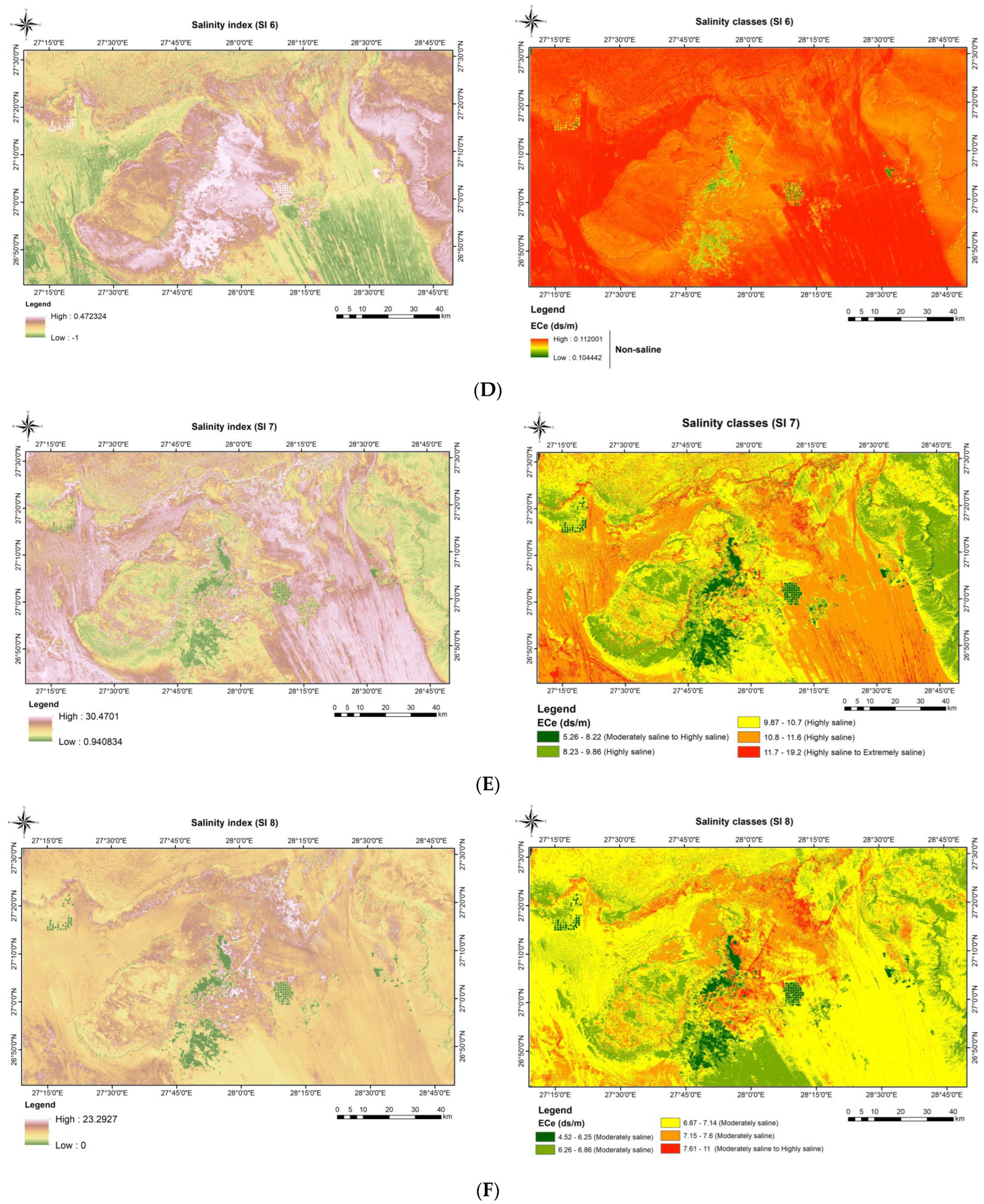
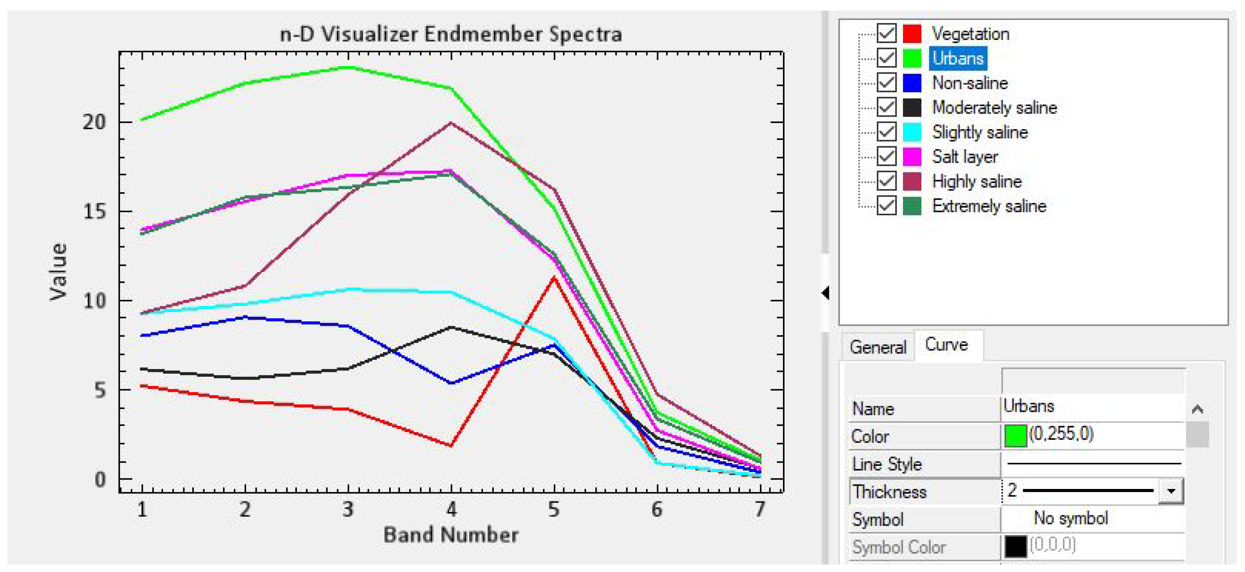
3.1. Estimation of Soil Salinity Based on Landsat-8 (OLI) Data and Soil Salinity Indices
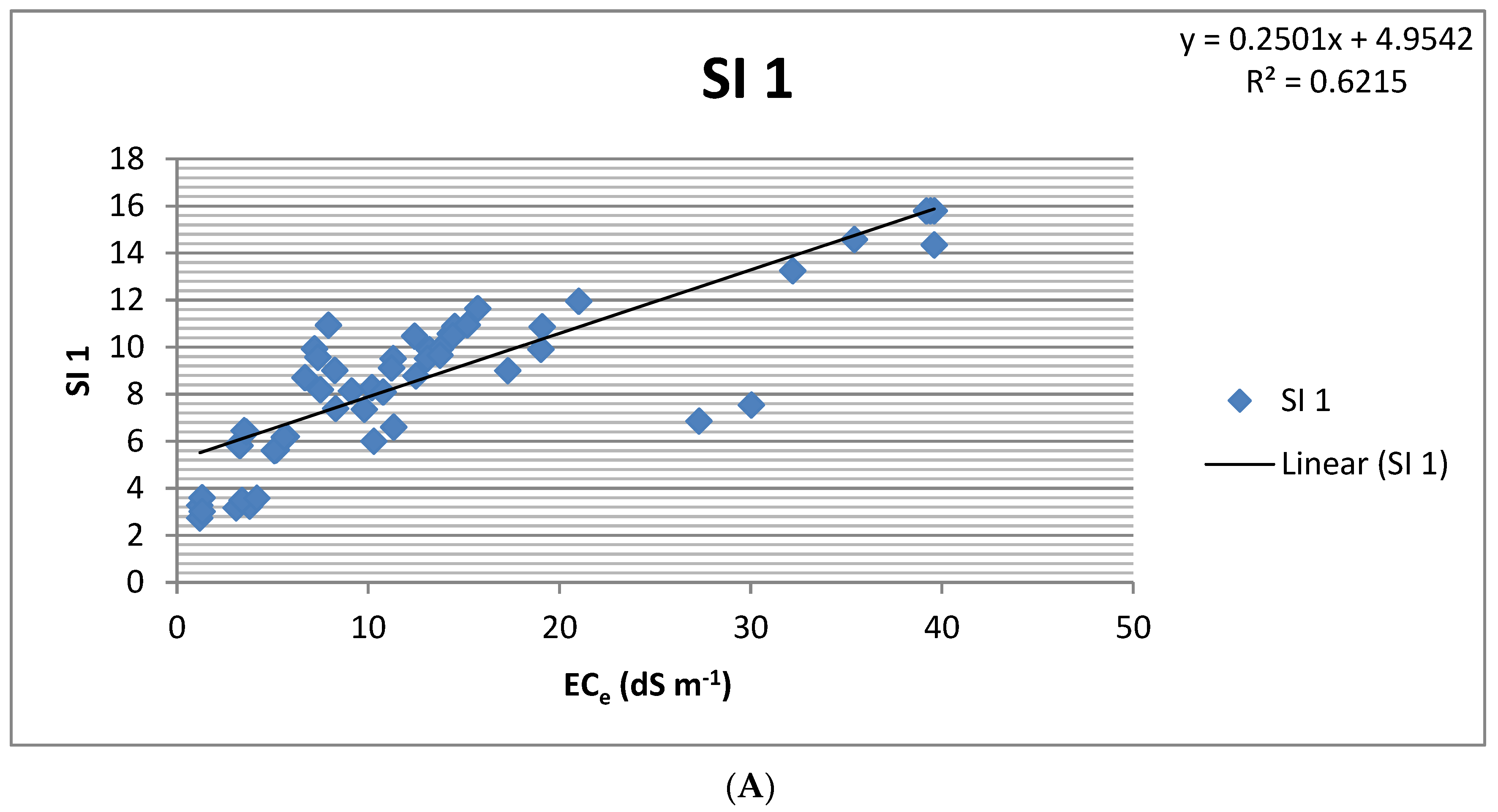
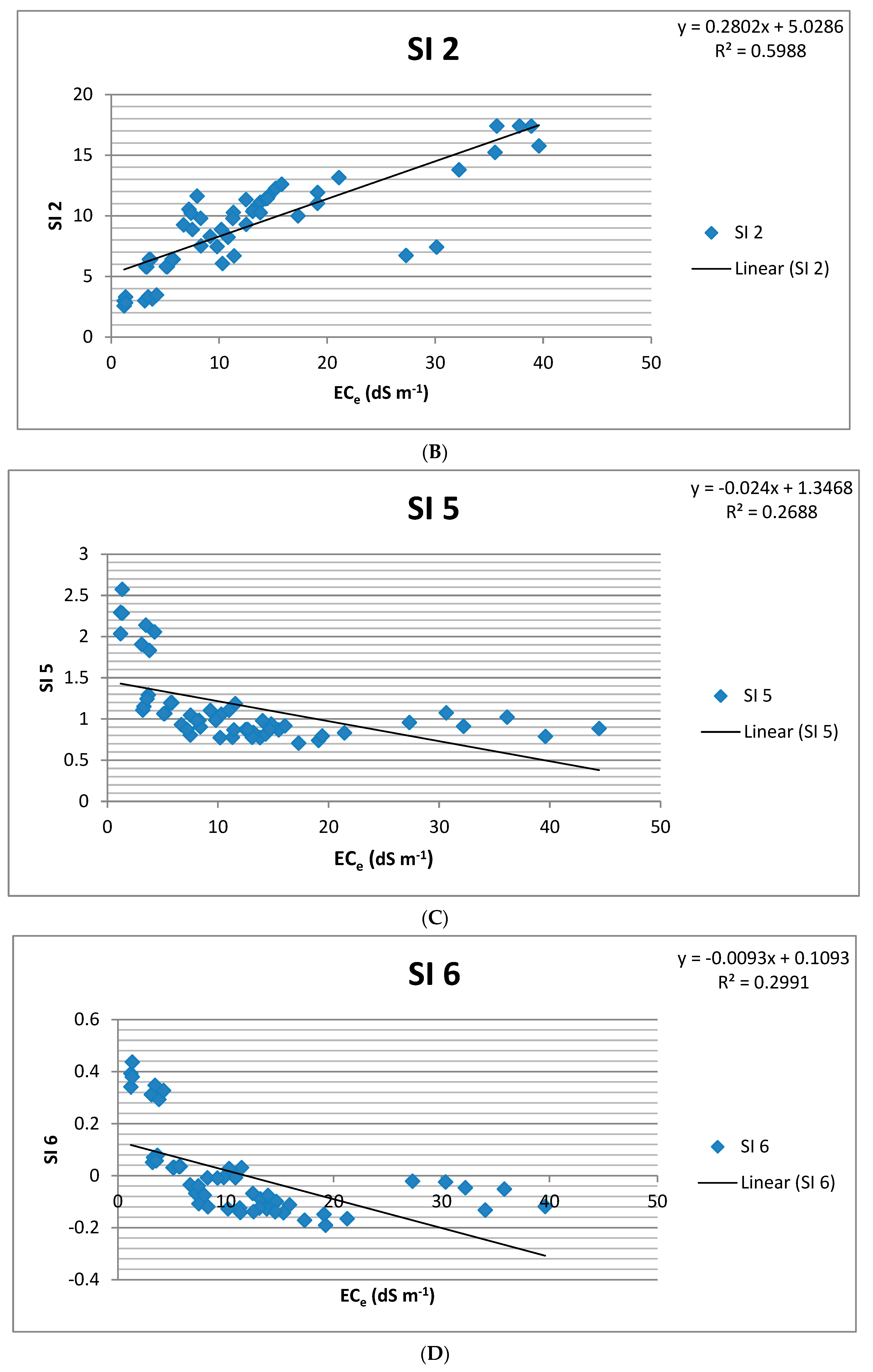
3.2. Devolved Linear Regression Model
3.3. Pearson Correlation Coefficient Analysis
3.4. Soil Salinity Values Prediction and Assessing Using Root Mean Square Error (RMSE)
3.5. Tukey’s Range, Significant and Difference Analysis (Model Validation)
4. Discussion
4.1. Estimation of Soil Salinization
4.2. Devolved Linear Regression Model
4.3. Pearson Correlation Coefficient Analysis
4.4. Soil Salinity Assessing Using Root Mean Square Error (RMSE)
4.5. Model Validation Using Tukey’s Test
5. Conclusions
Author Contributions
Funding
Institutional Review Board Statement
Informed Consent Statement
Data Availability Statement
Acknowledgments
Conflicts of Interest
References
- Gorji, T.; Sertel, E.; Tanik, A. Monitoring soil salinity via remote sensing technology under data scarce conditions: A case study from Turkey. Ecol. Indic. 2017, 74, 384–391. [Google Scholar] [CrossRef]
- Gorji, T.; Yildirim, A.; Hamzehpour, N.; Tanik, A.; Sertel, E. Soil salinity analysis of Urmia Lake Basin using Landsat-8 OLI and Sentinel-2A based spectral indices and electrical conductivity measurements. Ecol. Indic. 2020, 112, 106173. [Google Scholar] [CrossRef]
- Song, C.; Ren, H.; Huang, C. Estimating Soil Salinity in the Yellow River Delta, Eastern China—An Integrated Approach Using Spectral and Terrain Indices with the Generalized Additive Model. Pedosphere 2016, 26, 626–635. [Google Scholar] [CrossRef]
- Elhag, M.; Bahrawi, J.A. Soil salinity mapping and hydrological drought indices assessment in arid environments based on remote sensing techniques. Geosci. Instrum. Methods Data Syst. 2017, 6, 149–158. [Google Scholar] [CrossRef]
- Metternicht, G.I.; Zinck, J.A. Remote sensing of soil salinity: Potentials and constraints. Remote Sens. Environ. 2003, 85, 1–20. [Google Scholar] [CrossRef]
- Dwivedi, R.S. Soil resources mapping: A remote sensing perspective. Remote Sens. Rev. 2001, 20, 89–122. [Google Scholar] [CrossRef]
- Allbed, A.; Kumar, L. Soil salinity mapping and monitoring in arid and semi-arid regions using remote sensing technology: A review. Adv. Remote Sens. 2013, 2, 373–385. [Google Scholar] [CrossRef]
- Mohamed, E.S.; Belal, A.; Saleh, A. Assessment of land degradation east of the Nile Delta, Egypt using remote sensing and GIS techniques. Arab. J. Geosci. 2012, 6, 2843–2853. [Google Scholar] [CrossRef]
- Behera, S.K.; Shukla, A.K. Spatial distribution of surface soil acidity, electrical conductivity, soil organic carbon content and exchangeable potassium, calcium and magnesium in some cropped acid soils of India. Land Degrad. Dev. 2015, 26, 71–79. [Google Scholar] [CrossRef]
- Saleh, A.M.; Belal, A.B.; Mohamed, E.S. Land resources assessment of El-Galaba basin, South Egypt for the potentiality of agriculture expansion using remote sensing and GIS techniques. Egypt. J. Remote Sens. Space Sci. 2015, 18, S19–S30. [Google Scholar] [CrossRef]
- Saleh, A.M.; Belal, A.B.; Mohamed, E.S. Mapping of Soil Salinity Using Electromagnetic Induction: A Case Study of East Nile Delta, Egypt. Egypt. J. Soil Sci. 2017, 57, 167–174. [Google Scholar] [CrossRef]
- Abuzaid, A.S.; Abdellatif, A.D.; Fadl, M.E. Modeling soil quality in Dakahlia Governorate, Egypt using GIS techniques. Egypt. J. Remote Sens. Space Sci. 2021, 24, 255–264. [Google Scholar] [CrossRef]
- Jiapaer, G.; Chen, X.; Bao, A. A comparison of methods for estimating fractional vegetation cover in arid regions. Agric. For. Meteorol. 2011, 151, 1698–1710. [Google Scholar] [CrossRef]
- Soriano-Disla, J.M.; Janik, L.S.; Viscara Rossel, R.A.; Macdonald, L.M.; McLaughlin, M.J. The Performance of Visible, Near-, and Mid-Infrared Reflectance Spectroscopy for Prediction of Soil Physical, Chemical, and Biological Properties. Appl. Spectrosc. Rev. 2014, 49, 139–186. [Google Scholar] [CrossRef]
- Abuzaid, A.S.; AbdelRahman, M.A.E.; Fadl, M.E.; Scopa, A. Land Degradation Vulnerability Mapping in a Newly-Reclaimed Desert Oasis in a Hyper-Arid Agro-Ecosystem Using AHP and Geospatial Techniques. Agronomy 2021, 11, 1426. [Google Scholar] [CrossRef]
- Selmy, S.A.H.; Abd Al-Aziz, S.H.; Jiménez-Ballesta, R.; García-Navarro, F.J.; Fadl, M.E. Modeling and Assessing Potential Soil Erosion Hazards Using USLE and Wind Erosion Models in Integration with GIS Techniques Dakhla Oasis, Egypt. Agriculture 2021, 11, 1124. [Google Scholar] [CrossRef]
- Fadl, M.E.; Abuzaid, A.S.; AbdelRahman, M.A.E.; Biswas, A. Evaluation of Desertification Severity in El-Farafra Oasis, Western Desert of Egypt: Application of Modified MEDALUS Approach Using Wind Erosion Index and Factor Analysis. Land 2022, 11, 54. [Google Scholar] [CrossRef]
- Bartholomeus, K.L.; Antoine, S.; Martin, V.L.; Bas, V.W.; Ben-Dor, E.; Bernard, T. Soil organic carbon mapping of partially vegetated agricultural fields with imaging spectroscopy harm. Int. J. Appl. Earth Obs. Geoinf. 2011, 13, 81–88. [Google Scholar] [CrossRef]
- Stevens, A.; van-Wesemael, B.; Bartholomeus, H.; Tychon, B.; Ben-Dor, E. Laboratory, field and airborne spectroscopy for monitoring organic carbon content in agricultural soils. Geoderma 2008, 144, 395–404. [Google Scholar] [CrossRef]
- Weng, Y.; Gong, P.; Zhu, Z.-L. Soil sail content estimation in the Yellow River delta with satellite hyperspectral data. Can. J. Remote Sens. 2008, 34, 259–270. [Google Scholar]
- Ogen, Y.; Zaludab, J.; Francosb, N.; Goldshlegerc, N.; Ben-Dor, E. Cluster-based spectral models for a robust assessment of soil properties. Geoderma 2019, 340, 175–184. [Google Scholar] [CrossRef]
- Wold, S.; Sjöström, M.; Eriksson, L. PLS-regression: A basic tool of chemometrics. Chemom. Intell. Lab. Syst. 2001, 58, 109–130. [Google Scholar] [CrossRef]
- Woodcock, C.E. Uncertainty in remote sensing. In Uncertainty in Remote Sensing and GIS; Atkinson, P.M., Foody, G.M., Eds.; John Wiley & Sons: Hoboken, NJ, USA, 2003; pp. 19–24. ISBN 0-470-84408-6. [Google Scholar]
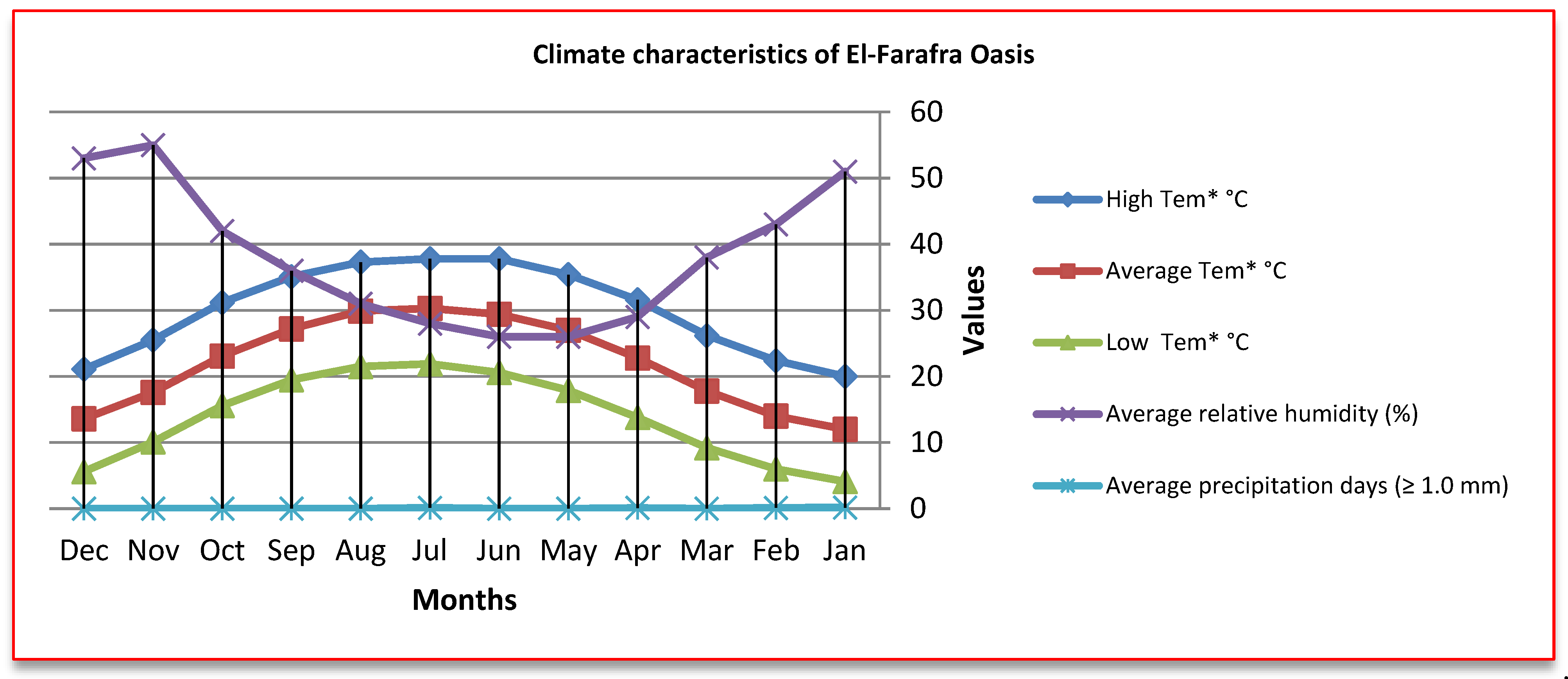
- National Oceanic and Atmospheric Administration (NOAA). El-Farafra Climate Normals"Appendix I: Meteorological Data". 2020. Available online: https://www.noaa.gov/ (accessed on 11 February 2022).
- Soil Survey Staff. Keys to Soil Taxonomy, 12th ed.; United States Department of Agriculture, Natural Resources Conservation Service: Washington, DC, USA, 2014; pp. 1–372.
- ENVI. ENVI User’s Guide. Software Package ver. 5.3.; Research Systems Inc.: Boulder, CO, USA, 2018; p. 1128. [Google Scholar]
- Esri Arc Map, version 10.2.2; Esri: Redlands, CA, USA, 2014.
- Soil Survey Staff. Soil Survey Laboratory Methods Manual. Soil Survey Investigations: Report 42, Version 4.0; United States Department of Agriculture, Natural Resources Conservation Service, National Soil Survey Center: Lincoln, NE, USA, 2004.
- Bashour, I.I.; Sayegh, A.H. Methods of Analysis for Soils of Arid and Semi-Arid Regions; FAO: Rome, Italy, 2007. [Google Scholar]
- Soil Survey Staff. Soil Survey Field and Laboratory Methods Manual: Soil Survey Investigations Report No. 51, Version 2.0; U.S. Department of Agriculture, Natural Resources Conservation Service: Washington, DC, USA, 2014; pp. 1–488.
- U.S. Salinity Laboratory Staff. Diagnosis and Improvement of Saline and Alkali Soils; Richards, L.A., Ed.; United States Department of Agriculture: Washington, DC, USA, 1954; Volume 60, pp. 1–166.
- Khan, N.M.; Rastoskuev, V.V.; Sato, Y.; Shiozawa, S. Assessment of hydrosaline land degradation by using a simple approach of remote sensing indicators. Agric. Water Manag. 2005, 77, 96–109. [Google Scholar] [CrossRef]
- Bannari, A.; Guedon, A.; El-Harti, A.; Cherkaoui, F.; El-Ghmari, A. Characterization of slightly and moderately saline and sodic soils in irrigated agricultural land using simulated data of advanced land imaging (EO-1) sensor. Commun. Soil Sci. Plant Anal. 2008, 39, 2795–2811. [Google Scholar] [CrossRef]
- Abbas, A.; Khan, S. Using Remote Sensing Techniques for Appraisal of Irrigated Soil Salinity. In International Congress on Modelling and Simulation (MODSIM); Oxley, L., Kulasiri, D., Eds.; Modelling and Simulation Society of Australia and New Zealand: Brighton, UK, 2007; pp. 2632–2638. [Google Scholar]
- Liu, Y.; Harding, A.; Gilbert, R.; Journal, A.G. A Workflow for Multiple-point Geostatistical Simulation. In Geostatistics Banff 2004; Leuangthong, O., Deutsch, C.V., Eds.; Springer: Dordrecht, The Netherlands, 2005; pp. 245–254. [Google Scholar]
- Jain, P.; Ramsankaran, R. GIS-based modelling of soil erosion processes using the modified-MMF (MMMF) model in a large watershed having vast agro-climatological differences. Earth Surf. Process. Landf. 2018, 43, 2064–2076. [Google Scholar] [CrossRef]
- Cohen, J. Statistical Power Analysis for the Behavioral Sciences, 2nd ed.; Routledge: New York, NY, USA, 1988. [Google Scholar] [CrossRef]
- Barnston, A.G. Correspondence among the correlation, RMSE, and Heidke forecast verification measures; refinement of the Heidke score. Weather. Forecast. 1992, 7, 699–709. [Google Scholar] [CrossRef]
- Tukey, J. Comparing individual means in the analysis of variance. Biometrics 1949, 5, 99–114. [Google Scholar] [CrossRef]
- Linton, L.; Harder, L. Biology 315–Quantitative Biology Lecture Notes; University of Calgary: Calgary, AB, Canada, 2007. [Google Scholar]
- Beek, K.J.; Blokhuis, W.A.; Driessen, P.M.; Van Breemen, N.; Brinkman, R.; Pons, L.J. Problem soils: Their reclamation and management. In Land Reclamation and Water Management, Developments, Problems and Challenges; International Institute for Land Reclamation and Improvement (ILRI): Wageningen, The Netherlands, 1980; pp. 43–72. [Google Scholar]
- Nawar, S.; Buddenbaum, H.; Hill, J.; Kozak, J. Modeling and mapping of soil salinity with reflectance spectroscopy and Landsat data using two quantitative methods (PLSR and MARS). Remote Sens. 2014, 6, 10813–10834. [Google Scholar] [CrossRef]
- Farifteh, J.; Van der Meer, F.; Atzberger, C.; Carranza, E. Quantitative analysis of salt-affected soil reflectance spectra: A comparison of two adaptive methods (PLSR and ANN). Remote Sens. Environ. 2007, 110, 59–78. [Google Scholar] [CrossRef]
- Yan, X.; Su, X. Linear Regression Analysis: Theory and Computing; World Scientific: Hackensack, NJ, USA, 2009; p. 328. [Google Scholar]
- Zhang, T.-T.; Qi, J.-G.; Gao, Y.; Ouyang, Z.-T.; Zeng, S.-L.; Zhao, B. Detecting soil salinity with MODIS time series VI data. Ecol. Indic. 2015, 52, 480–489. [Google Scholar] [CrossRef]
- Sidike, A.; Zhao, S.; Wen, Y. Estimating soil salinity in Pingluo County of China using QuickBird data and soil reflectance spectra. Int. J. Appl. Earth Obs. Geoinf. 2014, 26, 156–175. [Google Scholar] [CrossRef]
- Hammam, A.; Mohamed, E. Mapping soil salinity in the East Nile Delta using several methodological approaches of salinity assessment. Egypt. J. Remote Sens. Space Sci. 2020, 23, 125–131. [Google Scholar] [CrossRef]
- Kenney, J.F.; Keeping, E. Linear regression and correlation. Math. Stat. 1962, 1, 252–285. [Google Scholar]
- Zaidelman, F.R. Deep reclamation loosening of soils: State of the problem, results of research, prospects of application, and degradation changes. Eurasian Soil Sc. 2016, 49, 1061–1074. [Google Scholar] [CrossRef]
- Erkin, N.; Zhu, L.; Gu, H.; Tusiyiti, A. Method for predicting soil salinity concentrations in croplands based on machine learning and remote sensing techniques. J. Appl. Remote Sens. 2019, 13, 034520. [Google Scholar] [CrossRef]
- Fourati, H.T.; Bouaziz, M.; Benzina, M.; Bouaziz, S. Detection of terrain indices related to soil salinity and mapping salt-affected soils using remote sensing and geostatistical techniques. Environ. Monit. Assess. 2017, 189, 177. [Google Scholar] [CrossRef]


| Soil Salinity Classification | ECe (dSm−1) | Crop Yieldaffected |
|---|---|---|
| Non-saline | 0–2 | Not affected, salinity effects are negligible |
| Slightly saline | 2–4 | Sensitive crops affected, yield loss for very sensitive crops |
| Saline | 4–8 | Many crops were affected, and their yields restricted |
| Strongly saline | 8–16 | Only tolerant crops bear this condition |
| Extremely saline | >16 | A few very tolerant crops resist. |
| Satellite Data | Soil Salinityindices | Band Ratios | Description | References |
|---|---|---|---|---|
| Landsat-8 (OLI) | SI 1 | R =Band 4 = Red G = Band 3 = Green B = Band 2 = Blue NIR = Band 5 = Near Infra-Red | [32] | |
| SI 2 | ||||
| SI 5 | [33] | |||
| SI 6 | ||||
| SI 7 | ||||
| SI 8 | [34] | |||
| SI 9 |
| Descriptive Statistics | |||||
|---|---|---|---|---|---|
| ID | Number of Soil Samples | Minimum | Maximum | Mean | Std. Deviation |
| ECe (dS m−1) | 100 | 1.20 | 39.60 | 11.53 | 9.40 |
| SI 1 | 100 | 2.74 | 14.35 | 7.84 | 2.98 |
| SI 2 | 100 | 2.58 | 15.77 | 8.26 | 3.40 |
| SI 5 | 100 | 0.71 | 2.29 | 1.07 | 0.43 |
| SI 6 | 100 | −0.17 | 0.39 | 0.00 | 0.16 |
| SI 7 | 100 | 1.60 | 19.53 | 9.2 | 4.77 |
| SI 8 | 100 | 2.05 | 13.39 | 7.42 | 2.97 |
| SI 9 | 100 | 4.53 | 12.89 | 7.76 | 2.24 |
| Salinity Index | Index Range | Index Rangereference | Date of Satellite Image | Number of Samples | R2 |
|---|---|---|---|---|---|
| SI 1 | 0–1 | [1] | 8-December-2021 | 100 | 0.6215 |
| SI 2 | 0.5988 | ||||
| SI 5 | 0–1.73 | 0.2688 | |||
| SI 6 | 0–1.42 | 0.2991 | |||
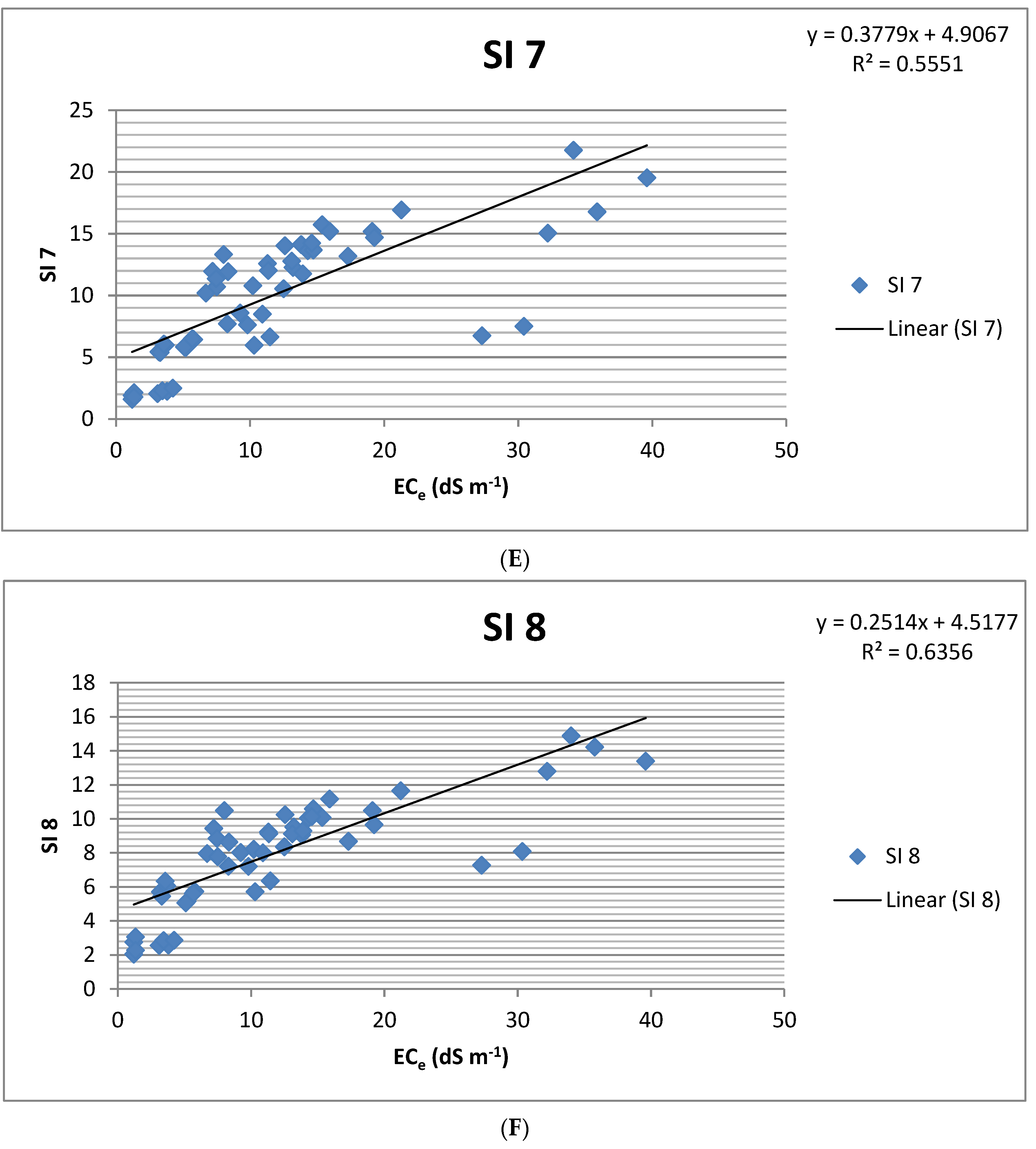
| SI 7 | 0.5551 | ||||
| SI 8 | 0.6356 | ||||
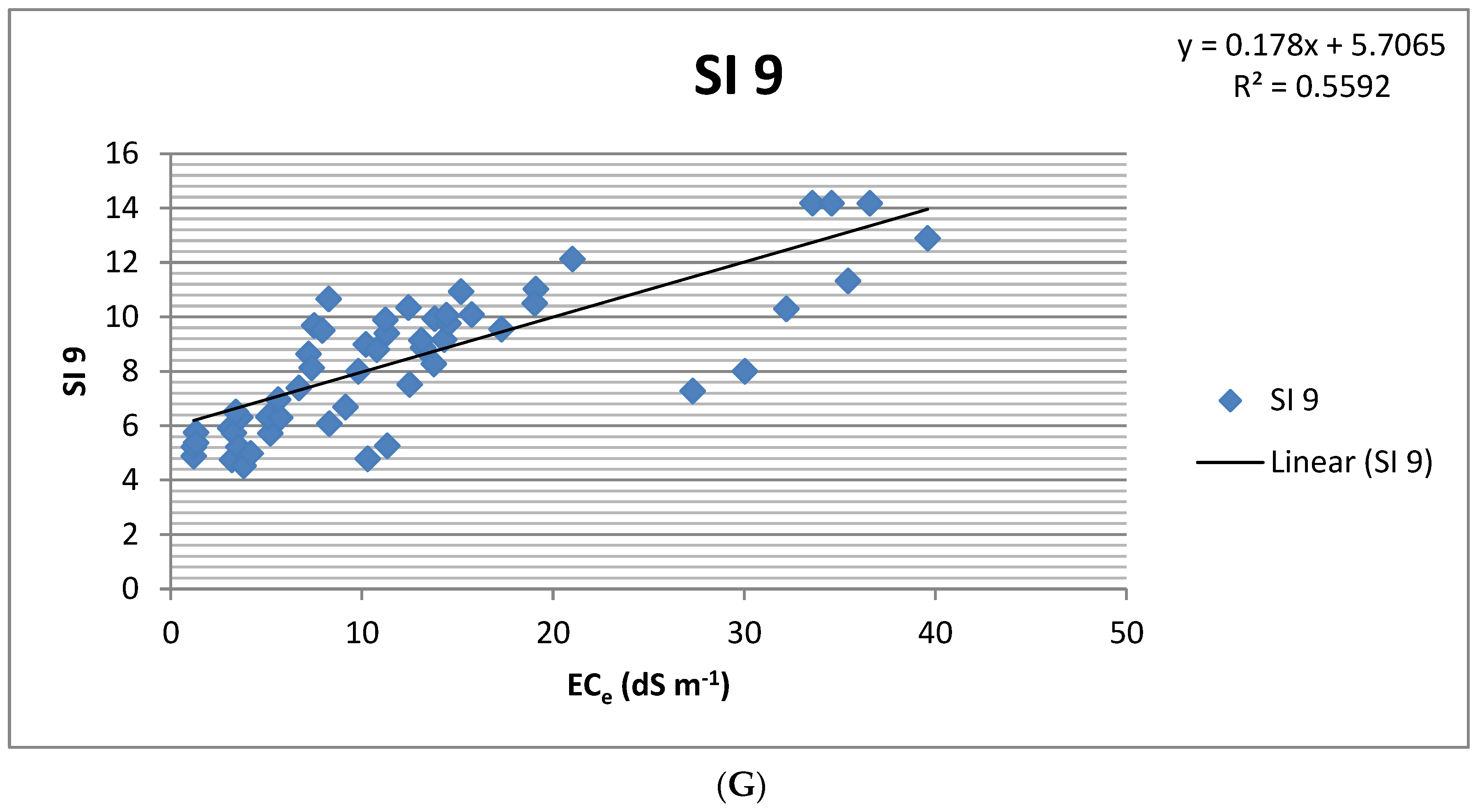
| SI 9 | 0.5592 |
| Pearson Correlations | ||||||||
|---|---|---|---|---|---|---|---|---|
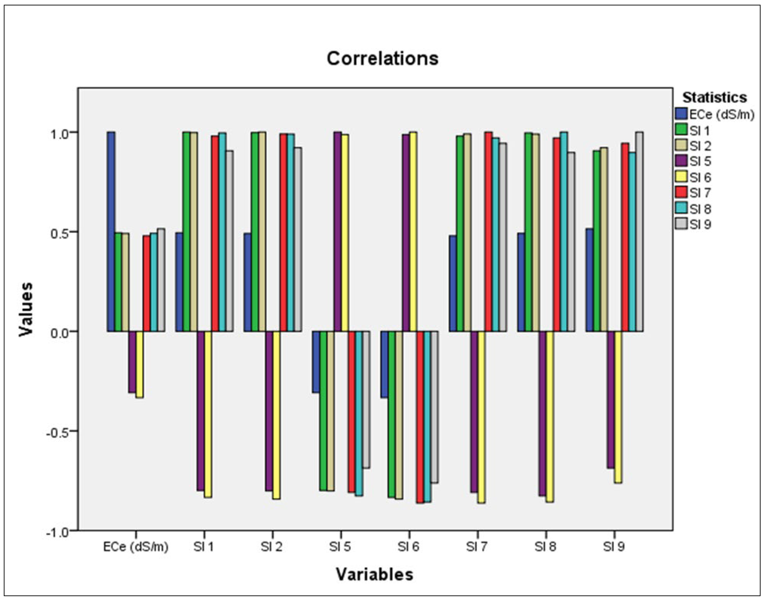
| ECe (dS m−1) | SI 1 | SI 2 | SI 5 | SI 6 | SI 7 | SI 8 | SI 9 | |
| ECe (dS m−1) | 1 | |||||||
| SI 1 | 0.495 * | 1 | ||||||
| SI 2 | 0.491 * | 0.998 ** | 1 | |||||
| SI 5 | −0.308 | −0.799 | −0.801 | 1 | ||||
| SI 6 | −0.333 | −0.833 | −0.842 | 0.988 ** | 1 | |||
| SI 7 | 0.479 * | 0.980 ** | 0.991 ** | −0.808 | −0.862 | 1 | ||
| SI 8 | 0.492 * | 0.996 ** | 0.990 ** | −0.826 | −0.857 | 0.971 ** | 1 | |
| SI 9 | 0.514 ** | 0.907 ** | 0.921 ** | −0.686 | −0.761 | 0.943 ** | 0.897 ** | 1 |
| Predict ECe (dS m−1) Salinity Values | |||||||
|---|---|---|---|---|---|---|---|
| SI 1 | SI 2 | SI 5 | SI 6 | SI 7 | SI 8 | SI 9 | |
| Minimum | 5.64 | 5.75 | 1.29 | 0.11 | 5.51 | 5.03 | 6.51 |
| Maximum | 8.54 | 9.45 | 1.33 | 0.11 | 12.29 | 7.88 | 8.00 |
| Mean | 5.64 | 5.75 | 1.29 | 0.11 | 5.51 | 5.03 | 6.51 |
| Std. deviation | 0.75 | 0.95 | 0.01 | 0.00 | 1.80 | 0.75 | 0.40 |
| Number of soil samples | 70 | 70 | 70 | 70 | 70 | 70 | 70 |
| RMSE | 9.81 | 9.49 | 13.75 | 14.68 | 8.58 | 10.07 | 9.98 |
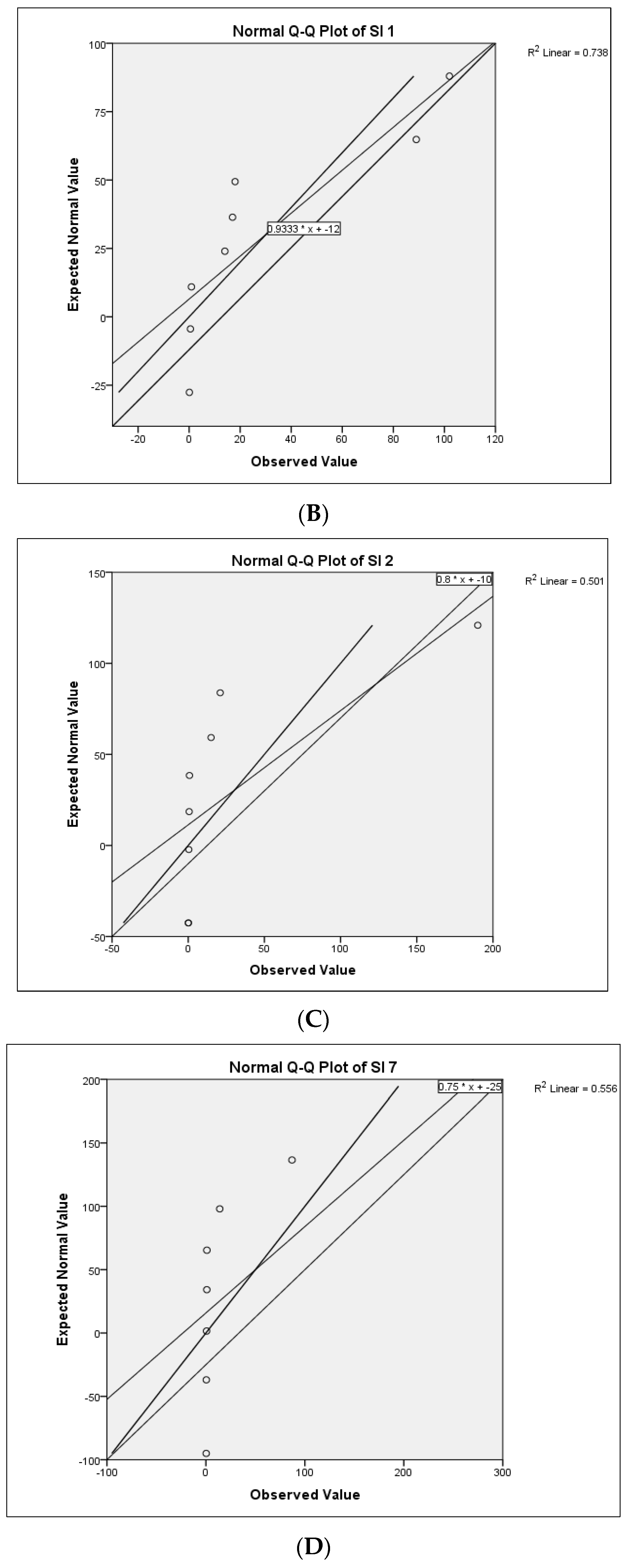
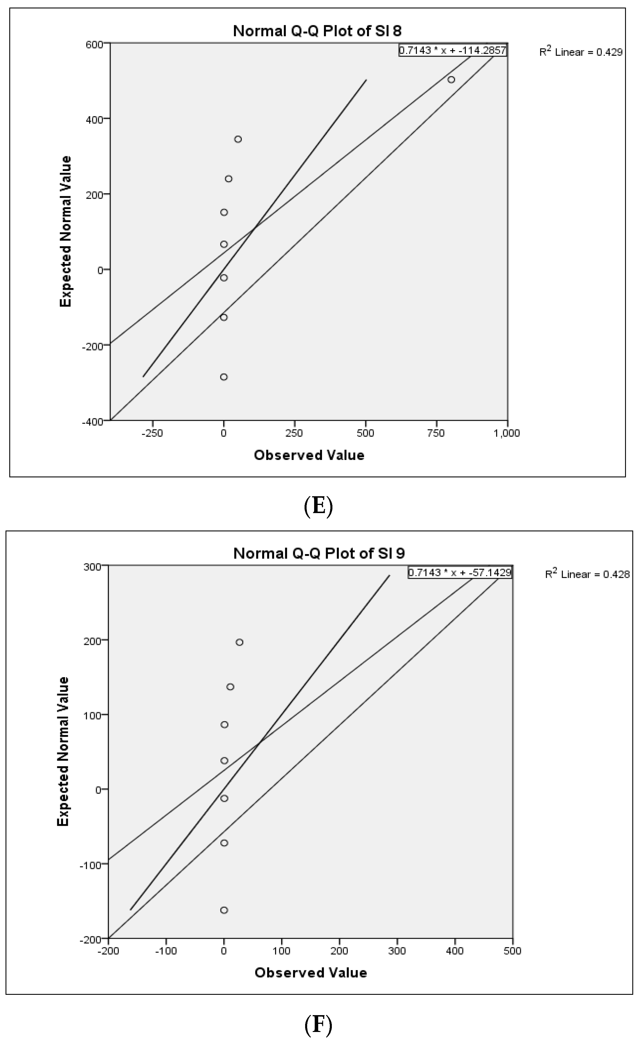
| Estimated Distribution Parameters | |||||||
|---|---|---|---|---|---|---|---|
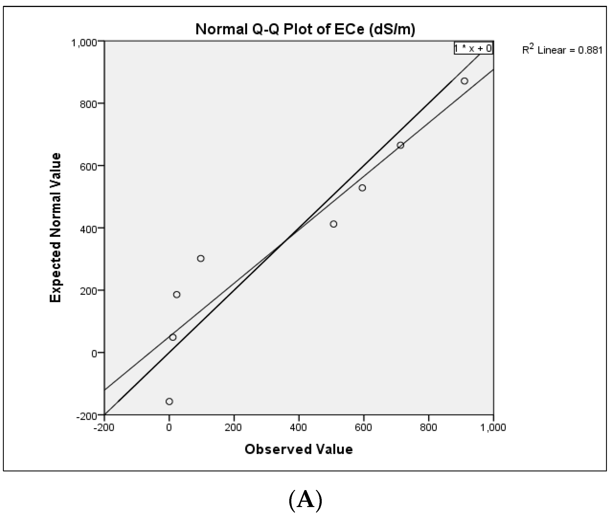
| ECe (dS m−1) | SI 1 | SI 2 | SI 7 | SI 8 | SI 9 | ||
| Normal Distribution | Observed mean | 8.123 | 8.215 | 9.443 | 2.121 | 9.502 | 11.288 |
| Expected mean | 9.735 | 1.946 | 3.040 | 1.110 | 3.246 | 4.598 | |
Disclaimer/Publisher’s Note: The statements, opinions and data contained in all publications are solely those of the individual author(s) and contributor(s) and not of MDPI and/or the editor(s). MDPI and/or the editor(s) disclaim responsibility for any injury to people or property resulting from any ideas, methods, instructions or products referred to in the content. |
© 2023 by the authors. Licensee MDPI, Basel, Switzerland. This article is an open access article distributed under the terms and conditions of the Creative Commons Attribution (CC BY) license (https://creativecommons.org/licenses/by/4.0/).
Share and Cite
Fadl, M.E.; Jalhoum, M.E.M.; AbdelRahman, M.A.E.; Ali, E.A.; Zahra, W.R.; Abuzaid, A.S.; Fiorentino, C.; D’Antonio, P.; Belal, A.A.; Scopa, A. Soil Salinity Assessing and Mapping Using Several Statistical and Distribution Techniques in Arid and Semi-Arid Ecosystems, Egypt. Agronomy 2023, 13, 583. https://doi.org/10.3390/agronomy13020583
Fadl ME, Jalhoum MEM, AbdelRahman MAE, Ali EA, Zahra WR, Abuzaid AS, Fiorentino C, D’Antonio P, Belal AA, Scopa A. Soil Salinity Assessing and Mapping Using Several Statistical and Distribution Techniques in Arid and Semi-Arid Ecosystems, Egypt. Agronomy. 2023; 13(2):583. https://doi.org/10.3390/agronomy13020583
Chicago/Turabian StyleFadl, Mohamed E., Mohamed E. M. Jalhoum, Mohamed A. E. AbdelRahman, Elsherbiny A. Ali, Wessam R. Zahra, Ahmed S. Abuzaid, Costanza Fiorentino, Paola D’Antonio, Abdelaziz A. Belal, and Antonio Scopa. 2023. "Soil Salinity Assessing and Mapping Using Several Statistical and Distribution Techniques in Arid and Semi-Arid Ecosystems, Egypt" Agronomy 13, no. 2: 583. https://doi.org/10.3390/agronomy13020583
APA StyleFadl, M. E., Jalhoum, M. E. M., AbdelRahman, M. A. E., Ali, E. A., Zahra, W. R., Abuzaid, A. S., Fiorentino, C., D’Antonio, P., Belal, A. A., & Scopa, A. (2023). Soil Salinity Assessing and Mapping Using Several Statistical and Distribution Techniques in Arid and Semi-Arid Ecosystems, Egypt. Agronomy, 13(2), 583. https://doi.org/10.3390/agronomy13020583