Abstract
“Crop-forcing” is an effective technique to delay grape maturation to a period of lower temperatures, and in this way, improve grape quality. Because of the aggressiveness of this technique (removal of leaves and fruit to reinitiate a second vegetative cycle), it may affect the level of reserves and could provoke progressive vine exhaustion. The aim of the present work is to evaluate the short- and medium-term evolution of carbohydrate reserves in different plant organs and the effect of “crop-forcing” under different irrigation regimes on seasonal biomass production and its distribution. The study was carried out over a four years period (2017–2020), applying “crop-forcing” in three consecutive years (2017–2019) to the same vines on two different dates and using two irrigation strategies. The application of “crop-forcing” did not decrease root reserve levels in either the year of application or the following year, but did modify starch and soluble sugar levels in shoots and leaves in some moments of the vegetative cycle during the years of “crop-forcing” application. Total biomass production in terms of grams per vine was lower in the “crop-forcing” treatments and continued to be so when “crop-forcing” was no longer applied. The percentage of biomass in vegetative organs increased at the expense of productive organs.
1. Introduction
The “crop-forcing” technique involves the application of a severe pruning when the vegetative period has begun, and the fruit-bearing buds of the following year are already formed. In this way, the cycle of the vines from budbreak is reinitiated with a consequent delay of the ripening cycle and transformation of the biannual reproductive cycle into an annual one. This technique was proposed by Gu et al. [1] and gave interesting results, delaying harvest to a period of more favorable temperatures. The most interesting aspect of this technique is that it is effective in improving some of the parameters that define the berries’ quality for red grape vinification, mainly those that are most affected by high temperatures or excess radiation during ripening. On the other hand, it increases production costs by introducing additional complex pruning and significantly reduces grape production. At present, it is difficult to believe that commercial vineyards are willing to adopt this technique as part of their usual practices, given the decrease in yields observed with this technique. However, the effect of climate change has sparked a growing interest in agronomic practices that can mitigate the negative consequences of rising temperatures in some of the main vineyard growing areas. This technique has been proposed as an interesting option for vineyards in warm regions, and as a strategy to combat the loss of grape quality caused by the extreme temperatures of global warming [1,2,3,4]. An aspect of undoubted practical interest that has not yet been studied is the effect of “crop-forcing” on the cumulative effect on the vines. Crop-forcing is an “aggressive” technique that modifies not only the timing of the phenology of the vine, but also the relationships between vegetative and productive organs, and therefore the source-sink relationships.
Each year, the vines have to initiate two reproductive cycles, an unfinished one that is interrupted with the forcing and one that takes place after the forcing. Non-structural carbohydrates (NSCs) are the energy source of the vine, composed of photassimilates synthesized in leaves (soluble carbohydrates) and reserves accumulated in the perennial woody organs of the previous year (starch) [5,6,7,8]. Thanks to the exchange of gases that takes place at leaf level throughout the canopy, these compounds are formed by photosynthesis through a reversible reaction, and are the source of energy required for vine growth in the moments when photosynthesis is not carried out. Glucose and fructose are the main products of photosynthesis and serve as raw material for the synthesis of sucrose and starch. Glucose and fructose synthesize sucrose in the leaves, which is transported to the rest of the plant as an energy source for growth [7]. The synthesis of starch commences when the synthesis of sucrose exceeds the amount that the vine can transport. Regulation of the formation of sucrose and starch depends on the ambient conditions and changes in the source–sink ratio [7]. Starch is the main carbohydrate stored in the vine [7], and is found in the roots and trunk [9,10,11]. This carbohydrate reserve is restored in the perennial organs through photosynthesis, which extends from flowering to leaf senescence [12,13]. Starch accumulation in the previous campaign is essential for the mobilization of reserves that act as a ‘source’ until photosynthesis commences [14,15]. After budbreak, the vine grows rapidly thanks to the energy provided by carbohydrates mobilized from the perennial organs during the beginning of spring [16,17,18,19,20], with the accumulation of carbohydrates therefore slow in the weeks following budbreak. When the leaves are sufficiently mature, the growth energy of the vine is based on photosynthesis, coinciding with the end of spring and beginning of summer, which is the period when the “crop-forcing” technique is applied. With this pruning, all leaves, inflorescences and part of the shoots are removed, as are also the reserves mobilized up to that moment from the roots and trunk to these organs. The vine has to restart the ‘forced’ budbreak under low carbohydrate availability, which explains the decrease in vigor of the campaign in course that could have a cumulative effect in following campaigns [21]. However, it has been shown in warm climates that the greatest accumulation of carbohydrates takes place in the post-harvest period [22,23]. Application of the “crop-forcing” technique might therefore modify grapevine carbohydrate accumulation as harvest is delayed in time to senescence, although very little has been studied in regards to this effect.
Agricultural practices can also modify the accumulation of reserves. Water stress reduces the rate of photosynthesis and can modify the distribution of assimilates in the vine. Differences between cultivars in their response to stress have been reported in the literature. Whereas water stress did not induce a diminution of carbohydrate reserves in ‘Garnacha’ and ‘Semillon’ [24], this was not the case in ‘Shiraz’ [25]. It can be assumed that aspects such as meteorological conditions and the moment and intensity of the water stress can also influence its impact on grapevine reserves.
According to the International Organisation of Vine and Wine (OIV) in 2021 the total vineyard area worldwide exceeded 7 million hectares, of which 13% is in Spain with more than 945,000 hectares. A large part of this area is located in semi-arid zones with high summer temperatures and low rainfall. For regions in hot areas, it is difficult to find a variety that adapts to the increase in temperature that is occurring [26]. High temperatures during the ripening period inhibit anthocyanin synthesis, reduce acidity and increase the alcohol content of wines. Predictions of maximum temperatures during the summer place different areas of Spain above 38 °C on average [27]. In Extremadura (Spain), the harvesting of ‘Tempranillo’ takes place from the end of August to the beginning of September. The application of “crop-forcing” at the pea size phenological stage has enabled grape maturation to be delayed to a time of milder temperatures and harvesting to mid-October, increasing total acidity and total polyphenol and anthocyanin content but with a fall in yield [4,28]. Use of the “crop-forcing” technique has been proposed in previous studies in combination with the application of a pre-veraison water deficit with the aim of achieving better results in terms of grape quality [29,30]; unpublished manuscript] and reducing the amount of irrigation water used. The aim of the present study is to analyze the short- and medium-term impact of “crop-forcing”, with and without the adoption of a controlled deficit irrigation strategy on the concentration of carbohydrates in the same vines over the course of the annual cycle, and for three consecutive years.
2. Materials and Methods
2.1. Location, Description of the Vineyard and Weather Conditions
The study was carried out in an experimental vineyard located at Badajoz, Extremadura, Spain (38°51′ N; 6°40′ W; 198 m) in a ‘Tempranillo’ vineyard (Vitis vinifera L.) grafted on Richter 110 rootstock, trained as bilateral cordons in a vertical trellis system with a drip irrigation system of 8 L/h per vine. The vines were 16 years old at the beginning of the study, and the cultivation practices were the usual ones in the area (besides the experimental treatments). All the vines were winter pruned to six spurs and two buds per spur. The rows are E-W oriented and row and vine spacing were 2.5 m and 1.2 m, respectively. In addition to winter pruning, the number of shoots per vine was adjusted manually in the spring (12 shoots per vine). The study was initiated in 2017, which was the year in which the first “crop-forcing” was applied, and which was repeated in 2018 and 2019. In 2020, only conventional pruning was carried out to evaluate the cumulative effect of this practice on the plants.
The soil is typical from the Guadiana River Valley, with a uniform, poorly differentiated profile. According to Soil Taxonomy (Soil Survey Staff 2006), this soil is in the order Entisol, suborder Orthent and in the great group Xerorthent. In general, these soils are slightly leached, with scarce calcium and with low sand adherence value. The upper soil has some humus content, while the lower soil is poor in it and also has a low nitrogen content. The vineyard soil was a silt-loam with 37.3% sand, 25.5% clay, 36.1% silt, and 1.1% organic matter (average depth 0.0 to 1.6 m). Volumetric water content was 0.30 m3/m3 at field capacity and 0.16 m3/m3 at the permanent wilting point.
The agrometeorological data were obtained from La Orden weather station (100 m from the vineyard) which forms part of the Agroclimatic Information System for Irrigation (SIAR by its initials in Spanish), with the characteristics described in Martí et al. [31].
2.2. Treatments and Experimental Design
The experimental design was a split plot with four replications (Table 1). The main factor was pruning with three treatments. Two of the treatments involved “crop-forcing” on different dates. In the F1 treatment, “crop-forcing” was applied three days after anthesis (18 May 2017; 29 May 2018; 20 May 2019) and in the F2 treatment 22 days after anthesis. Both treatments were compared with a treatment without forcing techniques (NF) with vines grown under conventional practices (just winter pruning). “Crop-forcing” consisted of hedging the growing shoots to seven nodes and removing all the summer laterals, leaves and clusters with scissors to force the bursting of the primary buds developed in the current season (Figure 1). The secondary factor was the irrigation strategy. Two treatments were assigned to the subplots: good water status (C), supplying water to maintain a midday stem water potential (SWP) close to −0.6 MPa (non-stressed), and a pre-veraison deficit irrigation treatment (RI) supplying water to reach a minimum SWP of −1.1 MPa and −0.8 MPa (low to moderate water stress) in post-veraison [32]. The experimental field design was kept intact for the first three years, and in 2020 only the irrigation treatments were applied.

Table 1.
Summary of the treatments applied in the study.
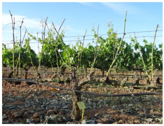
Figure 1.
‘Tempranillo’ vine subjected to “crop-forcing” in Extremadura.
Vine water requirements were calculated based on the crop evapotranspiration (ETc) using the crop coefficient (Kc) recommended by FAO for these latitudes for the NF treatments. For the F1 and F2 treatments, ETc was calculated directly on a weighing lysimeter [33] integrated in the study plot, using two F1 vines. Irrigation started when a threshold SWP value of −0.6 MPa was reached. Irrigation was applied five to six times per week, measuring the amount of water applied to each subplot with volumetric water meters and maintaining irrigation until the beginning or middle of October. The meteorological data were obtained from a weather station belonging to the Extremadura irrigation advisory network (REDAREX) which was located 100 m from the plot. The experimental unit comprised 6 rows per 18 vines. The ten central vines of the four central rows were used for sampling and harvested.
2.3. Vine Phenology and Water Status
A phenological assessment was performed weekly according to the modified E-L system [34]. A visual inspection was made of ten plants per plot, starting from mid-March (‘cotton bud’ stage), to determine the most representative growth stage (the stage shown by at least 50% of vines), as well as the most backward and the most advanced stages in the sample.
The SWP was measured at noon with a pressure chamber (Soil Moisture Corp., Model 3500, Santa Barbara, CA, USA), following the procedure described by Shackel et al. [35] using leaves on the north side of the trellis (in the shade) close to trunk level and wrapped in aluminum foil at least 2 h before data recording. Measurements were taken weekly on one leaf per vine and in two plants per subplot.
2.4. Production of Biomass
Yield dry weight vines were harvested by hand when the mean of the four replicates of each treatment reached total soluble solids (TSS) content of 23–24 °Brix (a common harvest criterion for this variety in this area). NF vines were harvested on 22 August 2017, 27 August 2018, 27 August 2019 and 5 August 2020. F1 vines were harvested on 12 September 2017, 8 October 2018, 30 September 2019 and 5 August 2020. F2 vines were harvested on 17 October 2017, 29 October 2018, 15 October 2019 and 5 August 2020. Clusters were cut, counted and weighed from a total of 10 vines per experimental plot.
Leaf dry weight/leaf area per vine was determined at harvest by multiplying the number of shoots per vine by the average leaf area of the shoot (LAS). LAS was estimated by measuring the area of all leaves of four shoots per experimental plot with a leaf area meter (LI-3100C, LI-COR Bioscience, Lincoln, NE, USA). Leaf dry weight per vine was then estimated from the leaf area to dry weight ratio (dry weight (g) = 0.0089 leaf area (cm2) − 1.651; r2 = 0.95) calculated for this variety under the same trial conditions. Leaf dry weight was estimated for 10 vines per experimental plot.
Dry weight of the pruning interventions/ten vines per experimental plot were selected, and dry weight was determined in the different interventions carried out: winter pruning, green pruning and forcing pruning only in the case of forced vines.
For all dry weight determinations, a forced ventilation stove was used to dry the samples at 65 °C until they reached a constant weight. A precision balance (Sartorius Mechatronics BP61S, Göttinger, Germany) with a sensitivity of 0.01 g was used to determine the dry weight.
2.5. Soluble Sugar Extraction and Starch Digestion
Root, shoot and leaf samples were collected from ten plants per subplot at different moments of the annual vine cycle. Root samples were collected in the 2017/2018, 2018/2019, 2019/2020 and 2020/2021 winters, and were washed with paper soaked in cold distilled water. Shoot samples were collected in the periods of winter pruning (2017, 2018 and 2019), bleeding sap (2019 and 2020), application of “crop-forcing” (2018 and 2019 only in the F1 and F2 treatments) and harvest (2018, 2019 and 2020). Leaf samples were collected in the periods of application of “crop-forcing” (2018 and 2019 only in F1 and F2 treatments), harvest (2018, 2019 and 2020) and leaf fall (2019 and 2020). A forced ventilation stove was used to dry the samples at 65 °C, and the samples were kept there until they reached a constant weight. Once dry, they were crushed to a fine powder (MF 10, Ika, Staufen, Germany). A sample of 50 mg was added to 10 mL of ethanol 80% and macerated for 10 min at 80 °C in a water bath (WNE, Memmert, Schwabach, Germany) and centrifuged for 5 min at 3000 rpm (5810, Eppendorf, Hamburg, Germany). The supernatant was separated and the resulting pellet was extracted up to three times. The supernatants (soluble sugar extracts) were then combined and stored at −20 °C.
The extraction of soluble sugars was carried out using a methodology based on a previous work [36]. A 5 mL aliquot of soluble sugar extract was dried and redissolved in 2 mL of H2Od for 5 min in an ultrasonic bath (USC-TH, VWR, Radnor, USA). The sample was macerated for 10 min at 80 °C in a water bath (WNE, Memmert, Schwabach, Germany) and centrifuged for 5 min at 3000 rpm (5810, Eppendorf, Hamburg, Germany). Determination of soluble sugar content from extracts (%Glu-Fru) was carried out using an autoanalyzer (Y15, Biosystems, Barcelona, Spain). Two extractions were performed for each sample of a given plot and sampling date.
The extraction of starch was carried out using a methodology based on a previous work [37]. Extracted sugar pellets were dried for 24 h (65 °C). 4 mL of sodium acetate (pH 4.6) was added and the mixture was macerated for 60 min at 100 °C (WNE, Memmert, Schwabach, Germany). The sample was cooled in a water-ice bath for 10 min. 1 mL of α-amylase was added and homogenized (ZX3, VELP, Monza and Brianza, Italy), macerated for 30 min at 85 °C and centrifugated for 5 min at 3000 rpm (5810, Eppendorf, Hambug, Germany). An aliquoted of 100 µL was added 500 µL of α- amyloglucosidase and homogenized (ZX3, VELP, Monza and Brianza, Italy) and macerated for 30 min at 60 °C. Determination of starch content from the extracts (%Starch) was carried out using an autoanalyzer (Y15, Biosystems, Barcelona, Spain). Two extractions were performed for each sample of a given plot and sampling date.
2.6. Statistical Data Analysis
Normality and homogeneity of variances were checked using the Shapiro-Wilk and Bartlett tests, respectively. When normality and homogeneity of variances were verified, the data were subjected to a multivariate analysis of variance (MANOVA) to investigate the effect of “crop-forcing”, “irrigation” and their interaction on each parameter evaluated, selecting p ≤ 0.001, p ≤ 0.01, and p ≤ 0.05 for significance of comparisons. The interaction between effects was evaluated by calculating the least-squares means (LS means), selecting p ≤ 0.001, p ≤ 0.01, and p ≤ 0.05 for significance of comparisons and the Tukey test as post hoc test for parametric samples. When normality and homogeneity of variance were not verified, non-parametric tests were carried out using the Kruskal–Wallis test (alternative to one-way ANOVA) and multiple comparison p values (alternative to post-hoc pairwise comparisons). Differences between means were considered statistically significant when p < 0.05. These statistical tests were performed with XLSTAT-Pro 201610 (Addinsoft, 2009, Paris, France).
The evolution data were statistically analyzed (SPSS Inc., Chicago, IL, USA) using the Shapiro–Wilks test as the test of normality, Levene’s test as the test of homogeneity of variances, with the one-factor ANOVA and the Tukey-B test and the t-Student test as parametric test, and Kruskal–Wallis’s test and multiple comparison p values and the Mann–Whitney U Test as nonparametric test. Differences between means were considered statistically significant when p < 0.05.
3. Results
3.1. Climatology, Phenology and Water Status
Figure 2 shows the seasonal evolution of maximum, minimum and mean temperature and monthly rainfall over the course of the 4 years of the study. Although the temperature pattern was similar in all years, 2018 saw the most spring and autumn rainfall of the three years in which “crop-forcing” was applied, as well as the highest temperatures in August. The year of highest rainfall was 2020.
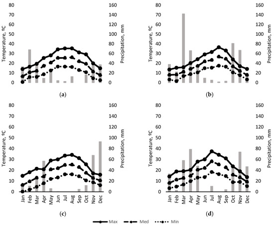
Figure 2.
Temperatures (lines), and rainfall (bars) during: (a) 2017; (b) 2018; (c) 2019 and (d) 2020.
While irrigation strategy did not modify vine phenology, “crop-forcing” did (Supplementary Table S1). The duration of the vegetative cycle reinitiated with the pruning in F1 and F2 was shortened in the three years of “crop-forcing” application, with all stages of the vegetative cycle reduced except for the veraison-to-harvest period in 2018. The shift in the growth cycle caused an increase in temperature in the initial stages of the new crop cycle, but the mean values were lower during ripening (veraison to harvest). Overall, mean, maximum and minimum temperatures from budbreak to harvest were higher in the treatments subjected to “crop-forcing” compared to those with conventional pruning (Figure 2).
Table 2 shows average SWP in each period of the growth season. In the first three years, all the “crop-forcing” treatments maintained SWP values between −0.45 and −0.73 MPa, indicating an absence of water stress before application of “crop-forcing”. Considering the entire vegetative cycle, the mean SWP values of the C treatments ranged between −0.41 and −0.82 MPa, with values for the C-F1 treatment between −0.45 and −0.89 MPa and for the C-F2 treatment between −0.42 and −0.79 MPa. The RI treatments supported a moderate water deficit in pre-veraison. The mean SWP of RI-NF was −1.00 MPa in this period, while for RI-F1 and RI-F2 the values were above −0.90 MPa in 2017 and 2018 and in 2019 did not exceed −0.80 MPa. In 2020, only very slight differences were found between the water status of the different treatments, despite maintaining the two irrigation strategies (C and RI), due to the abundant rains.
Table 2.
Average midday stem water potential (MPa) throughout the different phenological stages in 2017, 2018, 2019 and 2020. BB = Budbreak; CFP = “Crop-forcing” Pruning; F = Flowering; FS = Fruit Set; V = Veraison; H = Harvest; PostH = Postharvest.
3.2. Starch Content in Vegetative Organs
3.2.1. Roots
Figure 3 shows root starch concentration during winter dormancy in the 4 years from 2017/2018. There were significant differences between years, with the lowest concentrations in 2020/2021 and the highest in 2019/2020. However, in each year all the treatments had similar values, with no differences between pruning treatments for the same irrigation treatment (Figure 3a,b) or between irrigation treatments for the same pruning treatment.
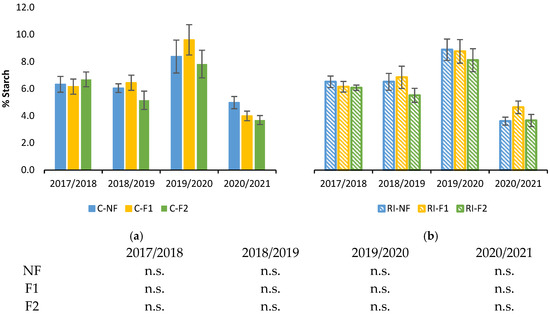
Figure 3.
Percentage of starch in relation to dry weight (%Starch) in roots during the winter dormancy period: (a) in C treatments C; (b) in RI treatments. The sample in each elementary plot corresponds to 10 plants. The figure shows the average of the 4 plots per treatment. Bars represent the standard error of the mean. Statistical analysis: ANOVA and Tukey test as parametric test and Kruskal–Wallis test as nonparametric test (both p < 0.05); n.s. indicates not significant.
3.2.2. Shoots (Winter Pruning)
Starch content in shoots pruned in winter was higher in 2019 than in the other years, as was also the case for roots (Supplementary Table S2).
Figure 4 shows the evolution of shoot starch content in different moments of the vegetative cycle from the winter pruning of 2018 to that of 2020. Starch content decreased from its highest levels in the winter pruning and after budbreak (moment of bleeding sap), with the lowest values corresponding to the samples collected in the “crop-forcing” pruning and with a subsequent recovery such that concentrations at harvest were similar to those of the winter pruning. The general pattern was similar in all treatments, although the F2 treatments had lower starch levels from the 2018 pruning to the 2019 “crop-forcing”. The NF and F1 treatments had similar concentrations throughout the samplings, except in the 2019 pruning when NF had a higher concentration. In 2020, all treatments showed similar starch concentrations (Supplementary Table S2).
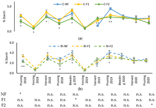
Figure 4.
Evolution of shoot starch percentage (%Starch) in: (a) C treatments; (b) RI treatments. The sample in each elementary plot corresponds to 10 plants. The figure shows the average of the 4 plots per treatment. Bars represent the standard error of the mean. The table indicates statistically significant differences between irrigation treatments for the same pruning treatment. Statistical analysis: ANOVA and the Tukey-B test and t-Student test as parametric test; Kruskal-Wallis’s test and multiple comparison p values and Mann–Whitney U test as nonparametric test. Differences between means were considered statistically significant when p < 0.05; n.s. indicates not significant; (*), significant at 5 percent level; (**), significant at 1 percent level.
Differences between the different irrigation treatments for the same pruning treatment were only observed in NF in the 2018 winter pruning, in F1 in the 2019 bleeding sap (both with higher values in C) and in F2 in the 2020 pruning (with higher values in RI).
3.2.3. Leaves
As can be seen in Figure 5, evolution of leaf starch content was similar in all treatments, although it was more stable in the case of C-NF along the different samplings. While certain seasonal variations were observed in the rest of the treatments, the same pattern was not repeated in the three years the samples were taken. In 2018 and 2020 the levels decreased at harvest, but not in 2019. In the absence of water stress, C-NF maintained high levels at all times and C-F2 the lowest levels, with intermediate values in F1. In RI, the three treatments maintained the same values, although there was a slight tendency to lower values in RI-F2. This tendency was not observed in 2020, when no “crop-forcing” was applied.
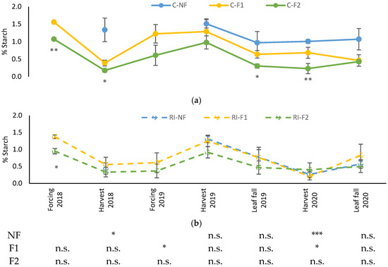
Figure 5.
Evolution of leaf starch percentage (%Starch) in: (a) C treatments; (b) RI treatments. The sample in each elementary plot corresponds to 10 plants. The figure shows the average of the 4 plots per treatment. Bars represent the standard error of the mean. The table indicates statistically significant differences between irrigation treatments for the same pruning treatment. Statistical analysis: ANOVA and the Tukey-B test and t-Student test as parametric test; Kruskal–Wallis’s test and multiple comparison p values and Mann–Whitney U test as nonparametric test. Differences between means were considered statistically significant when p < 0.05; n.s. indicates not significant; (*), significant at 5 percent level; (**), significant at 1 percent level and (***), significant at 0.1 percent level.
Differences between irrigation treatments for the same pruning treatment were observed in the 2018 harvest in NF, in the 2019 leaf fall in F1 and in the 2020 harvest in NF and F1. In all cases, the highest values were in C.
3.3. Soluble Sugar Content in Vegetative Organs
3.3.1. Roots
Figure 6 shows the percentage of soluble sugars in roots during the winter dormancy period for the four study years. As in the case of starch, no differences between forcing treatments were observed in any year, either in the C or RI treatments. As for the effect of irrigation for the same forcing treatment, statistically significant differences were only observed in the 2019/2020 winter for the NF treatments, with lower results in RI than in C (Figure 6).
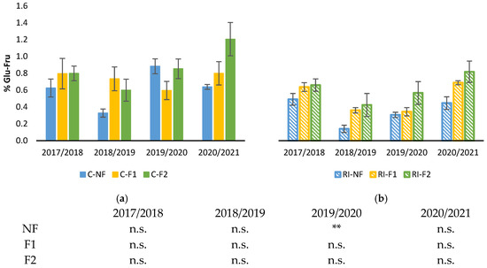
Figure 6.
Percentage of root soluble sugar content during the winter growth pause: (a) Percentage of soluble sugars (%Glu-Fru) in C treatments; (b) Percentage of soluble sugars (%Glu-Fru) in RI treatments. The sample in each elementary plot corresponds to 10 plants. The figure shows the average of the 4 plots per treatment. Bars represent the standard error of the mean. Statistical analysis: ANOVA and Tukey test as a parametric test and Kruskal–Wallis test as a nonparametric test (both p < 0.05); n.s. indicates not significant and (**) significant at 1 percent level.
3.3.2. Shoots
Shoot soluble sugar content at the time of winter pruning decreased year-on-year in all treatments. Significant interaction between irrigation and pruning was only observed in the 2019 harvest shoots. At winter pruning, differences were only observed in 2017, with higher values in RI than in C and in 2019 with higher concentrations in NF than in F1, and with intermediate values in F2. In the 2019 harvest there was interaction between the two effects, with differences in the C treatments (higher values in C-NF than in C-F1 and C-F2) but no differences in the RI treatments between RI-NF and RI-F1 and RI-F2. In 2020, the C treatments had higher soluble sugar content than the RI treatments. The effect of irrigation did not show any clear trend over the course of the study years (Supplementary Table S3).
The evolution of shoot glucose–fructose content is shown in Figure 7. The highest concentrations correspond to the winter dormancy period (winter pruning), which decreased to their minimum value in the bleeding sap stage, followed by a subsequent recovery in 2019 and 2020, but not in 2018. These evolutions in C showed no differences between pruning treatments until the 2019 harvest, when higher values were recorded for NF (Figure 7a). The trend was maintained until the 2020 bleeding sap stage, without differences between treatments from that moment onwards. Similar differences were not observed in RI. The only moment when differences between these treatments were observed was when applying “crop-forcing” in 2018 and 2019, with differences between F1 and F2, although not always in the same direction.
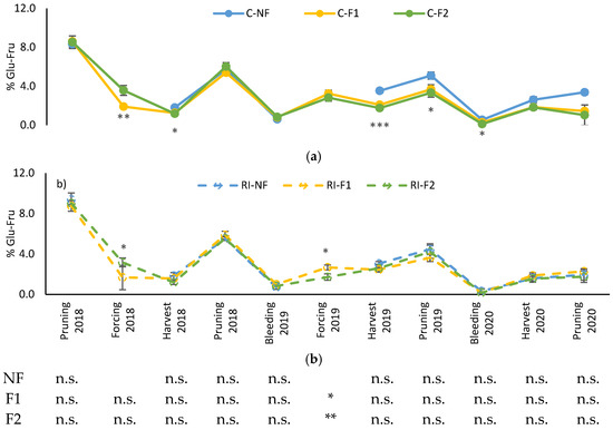
Figure 7.
Percentage of shoot soluble sugar content during the winter dormancy period: (a) Percentage of soluble sugars (%Glu-Fru) in C treatments; (b) Percentage of soluble sugars (%Glu-Fru) in RI treatments. The sample in each elementary plot corresponds to 10 plants. The figure shows the average of the 4 plots per treatment. Bars represent the standard error of the mean. The table indicates statistically significant differences between irrigation treatments for the same pruning treatment. Statistical analysis: ANOVA and the Tukey-B test and t-Student test as parametric test; Kruskal–Wallis’s test and multiple comparison p values and Mann–Whitney U test as nonparametric test. Differences between means were considered statistically significant when p < 0.05; n.s. indicates not significant; (*), significant at 5 percent level; (**), significant at 1 percent level and (***), significant at 0.1 percent level.
The only differences between irrigation treatments for the same pruning treatment were observed in the 2019 forcing in both F1 and F2, with higher values in C.
3.3.3. Leaves
Figure 8 shows the evolution of leaf glucose–fructose content. Levels were similar along the different samplings except for 2020. The evolution showed stable values, with higher accumulation found at 2020 leaf fall. In the C treatments, F2 maintained lower values of these sugars from the 2018 harvest to the 2019 harvest, followed by F1., while in 2020 the three treatments showed similar values. Differences between treatments in RI were only observed in the 2018 forcing.
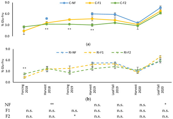
Figure 8.
Evolution of leaf soluble sugar content percentage (%Glu-Fru) in: (a) C treatments; (b) RI treatments. The sample in each elementary plot corresponds to 10 plants. The figure shows the average of the 4 plots per treatment. Bars represent the standard error of the mean. The table indicates statistically significant differences between irrigation treatments for the same pruning treatment. Statistical analysis: ANOVA and the Tukey-B test and t-Student test as parametric test; Kruskal–Wallis’s test and multiple comparison p values and Mann–Whitney U test as nonparametric test. Differences between means were considered statistically significant when p < 0.05; n.s. indicates not significant; (*), significant at 5 percent level; (**), significant at 1 percent level.
Differences between irrigation treatments for the same pruning treatment were only observed in the 2018 harvest in NF, in the 2019 forcing in F2, and in the 2020 leaf fall in NF. Again, the highest values were in C.
3.4. Biomass
Figure 9 shows total dry biomass produced by the vines of each treatment obtained as the sum of dry matter of yield, leaves and pruning interventions (winter pruning, green pruning and forcing pruning). During the forcing years (2017 to 2019) in the treatments with no water limitations C-NF obtained the highest biomass of the study, while in C-F2 the biomass was lower than in C-F1 in 2018 and 2019. In 2020, no differences were observed between C-NF and C-F1, but C-F2 had lower values. Additionally in 2020, C-NF obtained its lowest biomass, with weights lower than 2500 g/vine showing a notable interannual variability that was not observed in C-F1 and C-F2. In all the analyzed years, RI had lower total biomass production than C. Differences between pruning treatments were also lower than those observed in C.
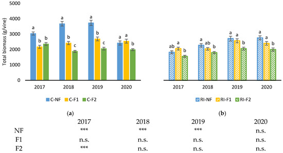
Figure 9.
Total biomass (g/vine) in: (a) C treatments; (b) RI treatments. The sample in each elementary plot corresponds to 10 plants. The figure shows the average of the 4 plots per treatment. Bars represent the standard error of the mean. The table indicates statistically significant differences between irrigation treatments for the same pruning treatment. Statistical analysis: ANOVA and the Tukey-B test and t-Student test as parametric test; Kruskal–Wallis’s test and multiple comparison p values and Mann–Whitney U test as nonparametric test. Differences between means were considered statistically significant when p < 0.05. Different letters indicate the existence of statistically significant differences between treatments; n.s., not significant; (***), significant at 0.1 percent level.
Among the non-forcing treatments, C-NF obtained higher values than RI-NF in 2017, 2018 and 2019, while in the forcing treatments C-F2 had higher values than RI-F2 only in 2017.
Figure 10 shows the percentage distribution of biomass (leaves, yield and pruning interventions). Biomass distribution for the same treatment was similar over the first three years. Generally, “crop-forcing” in both C and RI increased the proportion of pruning biomass at the expense of a reduction in biomass percentage (%) in yield and leaves in the case of F2.
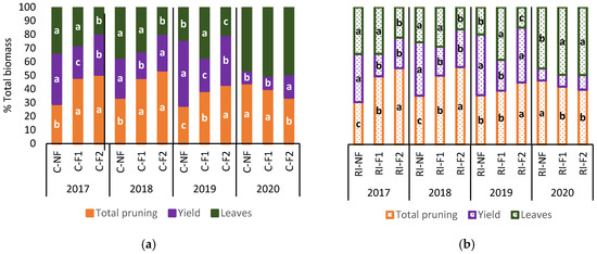
Figure 10.
Total biomass content (%) in leaves, yield and pruning interventions in: (a) C treatments; (b) RI treatments. The sample in each elementary plot corresponds to 10 plants. The figure shows the average of the 4 plots per treatment. Statistical analysis: ANOVA and Tukey test as a parametric test and Kruskal-Wallis test as a nonparametric test (both p < 0.05). Different letters indicate the existence of statistically significant differences between treatments.
F2 had a lower leaf biomass % in 2017, 2018 and 2019, while NF and F1 had similar leaf biomass % values in 2017 and 2018, with F1 increasing leaf biomass % compared to NF in 2019. In 2020, when no “crop-forcing” was applied, the deficit irrigation treatments of RI-F1 and RI-F2 saw a higher leaf biomass % than RI-NF. However, this effect was not observed between treatments with no water limitations (C-NF, C-F1 and C-F2). During 2017, 2018 and 2019 the lowest biomass % in yield was observed in C-F1, and in RI-F1 in 2020. Irrespective of irrigation treatment, F2 showed a lower yield biomass % than NF, except for C-F2 in 2018 and RI-F2 in 2019. In 2020, C-F2 had the highest yield biomass %, while no differences between treatments were observed in RI.
In 2020, the percentage distribution of biomass showed a similar trend in all treatments, with a significant decrease in yield biomass %, although with slight differences in C with the C-F2 treatment and in RI with the RI-NF treatment which do no not seem to be related to the pattern of the previous years.
Table 3 shows the biomass extracted in the different interventions. In the first three years, the highest yield biomass productions were observed in the NF treatments, especially in the C-NF treatment. The lowest were observed in F1 and F2 in 2017, 2018 and 2019. Application of RI decreased yield biomass significantly, except in 2018. Of the two forcing dates, F1 had lower yield biomass, although the differences were only statistically significant in RI in 2019. In 2018, 2019 and 2020, the amount of biomass produced as winter pruning in C-NF was higher than in the other treatments, followed by C-F1, RI-NF and RI-F1, while C-F2 and RI-F2 had the lowest values. In 2017, there was higher winter pruning biomass in C-NF, C-F1 and RI-F1 than in the other treatments. The biomass from the forcing pruning was higher in F2 than in F1 and only in 2017 were there differences between irrigation treatments, with more biomass extracted in C-F2 than in RI-F2. In the first three years, C-NF had the highest leaf biomass and F2 the lowest, with the differences being statistically significant. F1 had intermediate values compared to the other two pruning treatments (NF and F2), in both C and RI. The RI-NF and RI-F1 treatments had the same leaf biomass weights in 2017 and 2018.
Table 3.
Biomass in different organs during the years of “crop-forcing” application (2017, 2018, 2019) and the year of recovery (2020).
The green pruning data are shown in Table 3. This pruning was not carried out in 2017 in the F2 treatments. Interaction between the two effects was observed in 2017 and in 2018, while in 2019 differences were observed due to the effect of forcing and irrigation without interaction between the two. In 2017, a higher amount of matter removed in green pruning was observed in RI-F1 than in RI-NF, but these differences were not observed in C. In 2018, C-F2 had the lowest extracted material, with significant differences with respect to C-F1, RI-NF and RI-F1. In 2019, in the NF treatments the amount of removed material in the green pruning was lower than in F1 and F2. This value was also affected by the irrigation regime, with higher values in RI than in C.
Table 4 shows the ratio between dry weight and leaf area at harvest and between leaf area and leaf dry weight. Yield per leaf area unit of C-F2 was similar to that of C-NF in 2017 and 2018, and in 2018 and 2019 the RI-F2 values were similar to those of RI-NF. In the first three years, the F1 treatments had the lowest canopy yield in both C and RI. All treatments had similar values in 2020, although some differences were detected but with generally very low values due to the low grape yield as a result of damage caused by cryptogamic diseases. The most notable values observed in the leaf area to dry weight ratio (Table 4) were the high F2 values, principally for RI, with RI-F2 obtaining a better ratio than C-NF, RI-NF and RI-F1 in 2017 and than RI-NF in 2018. In 2019, C-F2 and RI-F2 had higher values than the rest of the treatments. In 2020, no differences were found between treatments.
Table 4.
Ratio between vine dry weight (Yield) and leaf area (LA) and ratio between leaf area and leaf dry weight (Leaves) during the years of “crop-forcing” application (2017, 2018, 2019) and during the year of recovery (2020).
4. Discussion
“Crop-forcing” is a severe pruning technique that modifies not only the phenology of the grapevine, but also the distribution of biomass among the vegetative and productive organs and hence the source–sink ratios. This work aims to provide information about how use of this technique can affect biomass distribution and vine reserve levels and, in this way, determine whether the technique may lead to premature vine exhaustion. This information is of particular importance for the establishment of systematic criteria for the application of this technique, should a commercial vineyard consider its benefits to be of interest in the achievement of its goals.
Carbohydrate reserves in roots, trunks and shoots play a vital role in the annual cycle of the grapevine and are determining factors for the vegetative and productive growth of the campaign in course, as well as those following given the biannual nature of the reproductive development of the grapevine. Low levels of reserves during the induction phase of the fruit-bearing buds that will bear fruit in the following campaign can reduce the potential number of inflorescences [38]. Budbreak and growth of shoots in their initial phase depend on the reserves accumulated at the end of the growth season of the previous year [39]. Additionally, this coincides with the phases of initiation and differentiation of inflorescences, when flower fertility of the campaign in course is determined and hence the number of berries per cluster. Through application of “crop-forcing”, with the removal of the recently formed photosynthetic cover (part of the shoots and all the leaves), the new budbreak takes place at the expense of some reserves partially consumed by the ‘natural’ budbreak. As can be seen in Figure 4, at the moment when the forcing pruning is performed, the shoots have lower starch, glucose and fructose content than at the moment of ‘natural’ budbreak, indicating a lower availability of carbohydrates to tackle bud regrowth. Similar results were found by Oliver-Manera et al. [40], who observed a lower total NSC concentration in the trunk at forcing date. However, the meteorological conditions of late spring, with its high temperatures, favored rapid shoot development and the development and expansion of photosynthetically active new leaves as well as canopy recovery, especially in F1 (data not shown). This allowed recovery of carbohydrates accumulated at harvest to levels similar to those observed in the previous winter pruning, as also observed by Oliver-Manera et al. [40] in a similar study in ‘Tempranillo’. Under our study conditions, the application of RI did not entail differences to those observed between F1 and F2 with respect to NF in the C treatments at any moment during the cycle, indicating that the application of RI together with forcing did not result in a greater exhaustion of reserves (Figure 3, Figure 4, Figure 5, Figure 6, Figure 7 and Figure 8). In addition, we found no evidence of a decrease in the grape’s sugar accumulation capacity on the dates studied; all treatments reached 24 °Brix (harvest criterion).
“Crop-forcing” shifts the vegetative cycle of the vine to a period of milder temperatures during grape maturation [1,2,3,4]. In warm climates, the greatest accumulation of carbohydrates in reserve organs takes place from post-harvest to leaf fall [22,23], and so the duration of this period can affect the synthesis of these compounds. Application of “crop-forcing” delayed harvest by up to two months, while the initiation of leaf fall took place on the same date for all treatments, reducing the post-harvest period in the “crop-forcing” treatments. In F1 and F2, leaf retention time on the vine was lower than in NF (Table S1), which was reflected in lower shoot starch concentrations during the winter dormancy period (Table S2) in both C and RI. However, this decrease was not observed in the roots (Figure 3), the main reserve organ of the grapevine [7,9,10,11].
With respect to root reserve levels, the characteristics of the year were more important than the pruning treatments applied. In view of the results of this work, it seems that importance should be given to the role of shoot reserve levels with respect to budbreak, as in F2, with similar root reserve levels, delays to budbreak were produced in 2018 and 2019, and in F1 in 2019, when shoot starch content was lower than in the NF treatments. In 2020, budbreak took place on the same date in all treatments, coinciding with the highest reserve levels being obtained in 2019. The break from dormancy is a complex and poorly understood process which, in addition to the influence of the carbohydrate reserves, it is believed may be associated with an increase in the production of hydrogen peroxide and the development of oxidative stress associated with low levels of catalase [38]. However, it is not unreasonable to acknowledge the possibility that budbreak delay was caused by lower accessibility to reserves.
The concentration of carbohydrates in leaves was more sensitive to application of the “crop-forcing” technique than the other organs which were analyzed, with the lower levels in F2 and the higher levels in NF being the most noteworthy results. It is probable that dominance of other sinks decreased leaf carbohydrate accumulation as they rapidly mobilized after photosynthetic assimilation. It should be noted that the leaves are perennial organs that cease to constitute a reserve for the vine with autumn leaf fall.
Water stress can accentuate the fall in vine reserve levels. Starch is the main reserve carbohydrate accumulated in grapevines [7,9,10]. Different studies have been conducted on the effect of the application of deficit irrigation strategies on starch accumulation. In ‘Garnacha’ and ‘Semillon’, water deficit resulted in decreased starch accumulation [24], but not in ‘Shiraz’ [25]. The results of the present work show that the application of water limitations in ‘Tempranillo’ did not, in general terms, result in a decrease in the starch or soluble sugars content in shoots or roots (Figure 3, Figure 4, Figure 5, Figure 6, Figure 7 and Figure 8 and Supplementary Tables S2 and S3), including when water limitations were applied to vines subjected to forcing.
As with the application of deficit irrigation, the forcing technique decreased the total biomass production of biomass. The biomass data show that delaying the forcing date resulted, in F2, in a higher proportion of biomass in vegetative organs that were removed with the pruning applications (Table 3), modifying the annual distribution of biomass (Figure 9). Due to this larger amount of removed dry matter, the F2 treatments always obtained the lowest leaf and pruned wood percentages (Figure 10), without exceeding NF either in yield percentage. This was not the case in F1 which, although it obtained lower yield and pruned wood percentages, had, in general lines, an increase in leaf percentage compared to the other two treatments (NF and F2).
In F2, leaf proportion was generally lower than in NF, but with leaves of lower density that could capture more solar radiation per gram of leaf, with the result that yield per leaf area unit was similar in F2 and NF. In F1, yield per leaf area unit was lower, as there was a greater proportional decrease in yield biomass than in leaf area. The F2 treatment was able to form clusters with mature berries that improved total acidity and anthocyanin content compared to the NF and F1 berries (articles in press).
It should be noted that, despite the decrease in total biomass as a result of “crop-forcing”, the values remained more or less stable over the course of the study in both the F1 and F2 treatments (Figure 9a,b), whereas in 2020 (when “crop-forcing” was not applied), a drastic reduction was observed in the NF treatments. This effect was due to the dramatic decrease in yield observed in 2020 caused by environmental conditions which favored cryptogamic diseases. Thus, the biomass distribution in 2020 was concentrated among pruned organs and leaves (Figure 10a,b), and differences were only observed with F2 in total biomass production. This result suggests that it is yield biomass that gives rise to the differences between the different pruning types, and that the rest of the organs are not as affected by “crop-forcing”, especially with F1. The source–sink balance favors biomass recovery and allows restoration of carbohydrate levels at the end of the season in the forcing treatments. Similar conclusions have been reported by Oliver-Manera et al. [40], with net carbon exchange rates per harvest unit around 2.5 times higher than in the non-forcing control treatment.
The results obtained in the present work show that the “crop-forcing” technique modifies NSC concentrations, principally in shoots and leaves, and that this is more evident in the case of the later forcing date. The differences established between F2 and the treatments with conventional winter pruning were maintained over the different years of the study, with no increase in the differences as the study progressed. In F1, as yield was reduced, photosynthetic assimilation was sufficient to maintain similar levels of reserves in the vine to NF. In F2, the lower canopy size and the short post-harvest period lowered reserves.
It does not therefore seem to be the case that “crop-forcing” results in progressive exhaustion, or that the deficit irrigation strategy causes cumulative exhaustion with “crop-forcing”. However, in 2020, when all the treatments were subjected to the same pruning, F2 had a lower number of clusters (17.4 clusters/vine in F2 against 22.3 and 22.5 in F1 and NF, respectively). This may be related to the lower carbohydrate content between budbreak and flowering, when induction of the following year’s flower buds takes place and the number of clusters is determined. As 2020 progressed the carbohydrate levels in all treatments tended towards similar values, and therefore a rapid recovery is expected in subsequent campaigns.
At the present time, it is difficult to believe, in view of the decline in yields observed with this technique, that commercial vineyards are willing to adopt it as a standard practice. The most interesting aspect is that it is effective in improving some of the parameters that define berry quality for winemaking, and therefore the value of the grape. Although it is evident that the practice of crop-forcing increases production costs, the mechanization of this practice could reduce the impact on the economic balance of the vineyard, which requires further development. Crop-forcing can also be an interesting technique to stagger the entry of grapes into the winery, combined with other techniques that cause shorter delays in harvest (late pruning, increased loads, etc.), as well as to “recover” vineyards that suffer biotic or abiotic damage in the initial stages after bud break.
5. Conclusions
In the three years in which the pruning treatments and irrigation strategies were applied, no clear symptoms were observed of progressive grapevine decline caused by the application of “crop-forcing”, water stress, or a combination of the two.
The date on which “crop-forcing” was applied was important in terms of shoot and leaf carbohydrate levels, which were lower throughout the season in the forcing treatment applied at a later date, compared to the treatment with conventional pruning and the earlier applied forcing treatment. With the forcing treatment applied at a later date, slight phenological deviations were observed. This could be related to the availability of carbohydrates over the course of the vegetative cycle, and in the recovery year the lower number of clusters per vine may be a first symptom of vine exhaustion.
Application of the “crop-forcing” technique decreased the seasonal production of biomass and modified its distribution among the different aerial organs. The deficit irrigation strategy, which induced water stress during pre-veraison, decreased biomass production, but did not result in modification of either biomass distribution among the different aerial parts of the vine or reserve levels of carbohydrates.
Supplementary Materials
The following supporting information can be downloaded at: https://www.mdpi.com/article/10.3390/agronomy13020395/s1, Table S1: Day of year of the different phenological states from budbreak to leaf fall in the different pruning treatments. Each pruning treatment represents the two irrigation treatments as no differences were found between them; Table S2: Shoot starch percentage during winter pruning and at harvest; Table S3: Percentage of shoot soluble sugar content during winter pruning and at harvest.
Author Contributions
Conceptualization, N.L., M.H.P. and D.U.; Data curation, N.L., M.H.P., D.U. and L.A.M.; Formal analysis, N.L., M.H.P., L.A.M. and D.U.; Funding acquisition, M.H.P.; Investigation, N.L., M.H.P., L.A.M., D.U. and M.E.V.; Methodology, N.L., M.H.P., D.U., L.A.M., M.E.V. and D.M.; Project administration, M.H.P.; Resources, M.H.P. and D.U.; Software, N.L. and D.U.; Supervision, N.L., M.H.P., D.U. and M.E.V.; Writing original draft, N.L., M.H.P. and D.U.; Writing, review & editing, N.L., M.H.P. and D.U. All authors have read and agreed to the published version of the manuscript.
Funding
This research was supported by funds from INIA Project RTA-2015-00089-C02-01, the ERDF, Junta de Extremadura, AGA001 (GR21196) and AGROS2022. N. Lavado was supported by FPI-INIA CPD2016-0081.
Institutional Review Board Statement
Not applicable.
Informed Consent Statement
Not applicable.
Data Availability Statement
All data supporting these results have been included in this manuscript.
Acknowledgments
The authors would like to thank Eva María Sereno for technical support.
Conflicts of Interest
The authors declare no conflict of interest.
References
- Gu, S.; Jacobs, S.D.; McCarthy, B.S.; Gohil, H.L. Forcing vine regrowth and shifting fruit ripening in a warm region to enhance fruit quality in “Cabernet Sauvignon” grapevine (Vitis vinifera L.). J. Hortic. Sci. Biotechnol. 2012, 87, 287–292. [Google Scholar] [CrossRef]
- Kishimoto, M.; Yamamoto, T.; Kobayashi, Y. Effects of Lateral or Secondary Induced Shoot Use on Number of Bunches and Fruit Quality in Forcing Cultivation by Current Shoot Cutting and Flower Cluster Removal to Shift Grape Ripening to a Cooler Season. Hortic. J. 2022, 91, 169–175. [Google Scholar] [CrossRef]
- Martínez-Moreno, A.; Sanz, F.; Yeves, A.; Gil-Muñoz, R.; Martínez, V.; Intrigliolo, D.S.; Buesa, I. Forcing bud growth by double-pruning as a technique to improve grape composition of Vitis vinifera L. cv. Tempranillo in a semi-arid Mediterranean climate. Sci. Hortic. 2019, 256, 108614. [Google Scholar] [CrossRef]
- Martinez De Toda, F.; Garcia, J.; Balda, P. Preliminary results on forcing vine regrowth to delay ripening to a cooler period. Vitis J. Grapevine Res. 2019, 58, 17–22. [Google Scholar]
- Lebon, G.; Wojnarowiez, G.; Holzapfel, B.; Fontaine, F.; Vaillant-Gaveau, N.; Clément, C. Sugars and flowering in the grapevine (Vitis vinifera L.). J. Exp. Bot. 2008, 59, 2565–2578. [Google Scholar] [CrossRef]
- Loescher, W.H.; Mccamant, T.; Keller, J.D. Carbohydrate Reserves, Translocation, and Storage in Woody Plant Roots. HortSci. 1990, 25, 274–281. [Google Scholar] [CrossRef]
- Mullins, M.G.; Bouquet, A.; Williams, L.E. Biology of the Grapevine; Cambridge University Press: London, UK, 1992; p. 239. [Google Scholar]
- Zapata, C.; Magne, C.; Deléens, E.; Brun, O.; Audran, J.C.; Chaillou, S. Grapevine culture in trenches: Root growth and dry matter partitioning. Aust. J. Grape Wine Res. 2001, 7, 127–131. [Google Scholar] [CrossRef]
- Köse, B.; Ateş, S. Saisonale Veränderungen von Kohlenhydratgehalten im Spross und Wachstumseigenschaften bei der Rebsorte ‘Trakya İlkeren’ (Vitis vinifera L.). Erwerbs Obstbau. 2017, 59, 61–70. [Google Scholar] [CrossRef]
- Pellegrino, A.; Clingeleffer, P.; Cooley, N.; Walker, R. Management practices impact vine carbohydrate status to a greater extent than vine productivity. Front. Plant Sci. 2014, 5, 1–13. [Google Scholar] [CrossRef]
- Zapata, C.; Deléens, E.; Chaillou, S.; Magné, C. Mobilisation and distribution of starch and total N in two grapevine cultivars differing in their susceptibility to shedding. Funct. Plant Biol. 2004, 31, 1127–1135. [Google Scholar] [CrossRef]
- Candolfi-Vasconcelos, M.C.; Candolfi, M.P.; Kohlet, W. Retranslocation of carbon reserves from the woody storage tissues into the fruit as a response to defoliation stress during the ripening period in Vitis vinifera L. Planta 1994, 192, 567–573. [Google Scholar] [CrossRef]
- Chaumont, M.; Foyer, C.H. Seasonal and diurnal changes in photosynthesis and carbon partitioning in Vitis vinifera leaves in vines with and without fruit. J. Exp. Bot. 1994, 45, 1235–1243. [Google Scholar] [CrossRef]
- Smith, J.P.; Holzapfel, B.P. Cumulative responses of semillon grapevines to late season perturbation of carbohydrate reserve status. Am. J. Enol. Vitic. 2009, 60, 461–470. [Google Scholar] [CrossRef]
- Zapata, C.; Deléens, E.; Chaillou, S.; Magné, C. Partitioning and mobilization of starch and N reserves in grapevine (Vitis vinifera L.). J. Plant Physiol. 2004, 161, 1031–1040. [Google Scholar] [CrossRef]
- Conradie, W.J. Seasonal Uptake of Nutrients by Chenin Blanc in Sand Culture: II. Phosphorus, Potassium, Calcium and Magnesium. S. Afr. J. Enol. Vitic. 1980, 2, 1978–1981. [Google Scholar] [CrossRef]
- Hale, C.R.; Weaver, R.J. The effect of developmental stage on direction of translocation of photosynthate in Vitis vinifera. Hilgardia 1962, 33, 89–131. [Google Scholar] [CrossRef]
- Kriedemann, P.E.; Kuewer, W.M. Leaf age and photosynthesis in Vitis vinifera L. Irrig. Insights 1970, 104, 97–104. [Google Scholar]
- Scholefield, P.; Neales, T.; May, P. Carbon Balance of the Sultana Vine (Vitis vinifera L.) And the Effects of Autumn Defoliation by Harvest-Pruning. Funct. Plant Biol. 1978, 5, 561. [Google Scholar] [CrossRef]
- Weyand, K.M.; Schultz, H.R. Long-term dynamics of nitrogen and carbohydrate reserves in woody parts of minimally and severely pruned Riesling vines in a cool climate. Am. J. Enol. Vitic. 2006, 57, 172–182. [Google Scholar] [CrossRef]
- Poni, S.; Gatti, M.; Tombesi, S.; Squeri, C.; Sabbatini, P.; Lavado Rodas, N.; Frioni, T. Double cropping in vitis vinifera l. pinot noir: Myth or reality? Agronomy 2020, 10, 799. [Google Scholar] [CrossRef]
- Bennett, J.; Jarvis, P.; Creasy, G.; Trought, M. Influence of Defoliation on Overwintering Carbohydrate Reserves, Return Bloom, and Yield of Mature Chardonnay Grapevines. Am. J. Enol. Vitic. 2005, 56, 386–393. [Google Scholar] [CrossRef]
- Vaillant-Gaveau, N.; Wojnarowiez, G.; Petit, A.N.; Jacquens, L.; Panigai, L.; Clément, C.; Fontaine, F. Relationships between carbohydrates and reproductive development in chardonnay grapevine: Impact of defoliation and fruit removal treatments during four successive growing seasons. J. Int. Sci. Vigne Vin. 2014, 48, 219–229. [Google Scholar] [CrossRef]
- Rogiers, S.Y.; Holzapfel, B.P.; Smith, J.P. Sugar accumulation in roots of two grape varieties with contrasting response to water stress. Ann. Appl. Biol. 2011, 159, 399–413. [Google Scholar] [CrossRef]
- Holzapfel, B.P.; Smith, J.P.; Field, S.K.; James Hardie, W. Dynamics of Carbohydrate Reserves in Cultivated Grapevines. Hortic. Rev. 2010, 37, 143–211. [Google Scholar]
- Jones, G.V. Climate and terroir: Impacts of climate variability and change on wine. In Fine Wine and Terroir—The Geoscience Perspective; Geoscience Canada Reprint; Macqueen, R.W., Meinerts, L.D., Eds.; Geological Association of Canada: St. John’s, NL, Canada, 2006; p. 247. [Google Scholar]
- Transición Ministerio para la Transición Ecológica y el reto Demográfico. Plataforma sobre Adaptación al Cambio Climático en España. Available online: http://escenarios.adaptecca.es/#&model=EURO-CORDEX (accessed on 24 January 2022).
- Lavado, N.; Uriarte, D.; Mancha, L.A.; Moreno, D.; Valdés, E.; Prieto, M.H. Effect of forcing vine regrowth on ’Tempranillo’ (Vitis vinifera L.) berry development and quality in Extremadura. Vitis 2019, 58, 135–142. [Google Scholar]
- Lavado, N.; Uriarte, D.; Mancha, L.A.; Moreno, D.; Valdés, M.E.; Prieto, M.H. Assessment of the crop forcing technique and irrigation strategy on the ripening of Tempranillo grapes in a semi-arid climate. 2023; Under Review. [Google Scholar]
- Lavado, N.; Prieto, M.H.; Mancha, L.A.; Moreno, D.; Valdés, M.E.; Uriarte, D. Combined effect of crop forcing and reduced irrigation as techniques to delay the ripening and improve the quality of ’Tempranillo’ (Vitis vinifera L.) berries in semi-arid climate conditions. 2023; Under Review. [Google Scholar]
- Martí, P.; González-Altozano, P.; López-Urrea, R.; Mancha, L.A.; Shiri, J. Modeling reference evapotranspiration with calculated targets. Assessment and implications. Agric. Water Manag. 2015, 149, 81–90. [Google Scholar] [CrossRef]
- van Leeuwen, C.; Tregoat, O.; Choné, X.; Bois, B.; Pernet, D.; Gaudillére, J.P. Vine water status is a key factor in grape ripening and vintage quality for red bordeaux wine. How can it be assessed for vineyard management purposes? J. Int. Sci. Vigne Vin. 2009, 43, 121–134. [Google Scholar] [CrossRef]
- Picón-Toro, J.; González-Dugo, V.; Uriarte, D.; Mancha, L.A.; Testi, L. Effects of canopy size and water stress over the crop coefficient of a “Tempranillo” vineyard in south-western Spain. Irrig. Sci. 2012, 30, 419–432. [Google Scholar] [CrossRef]
- Coombe, B.G. Growth Stages of the Grapevine: Adoption of a system for identifying grapevine growth stages. Aust. J. Grape Wine Res. 1995, 1, 104–110. [Google Scholar] [CrossRef]
- Shackel, K.A.; Ahmadi, H.; Biasi, W.; Buchner, R.; Goldhamer, D.; Gurusinghe, S.; Hasey, J.; Kester, D.; Krueger, B.; Lampinen, B.; et al. Plant Water Status as an Index of Irrigation Need in Deciduous Fruit Trees. HortTechnology 1997, 7, 23–29. [Google Scholar] [CrossRef]
- Landhäusser, S.M.; Chow, P.S.; Turin Dickman, L.; Furze, M.E.; Kuhlman, I.; Schmid, S.; Wiesenbauer, J.; Wild, B.; Gleixner, G.; Hartmann, H.; et al. Standardized protocols and procedures can precisely and accurately quantify non-structural carbohydrates. Tree Physiol. 2018, 38, 1764–1778. [Google Scholar] [CrossRef] [PubMed]
- Quentin, A.G.; Pinkard, E.A.; Ryan, M.G.; Tissue, D.T.; Baggett, L.S.; Adams, H.D.; Maillard, P.; Marchand, J.; Landhäusser, S.M.; Lacointe, A.; et al. Non-structural carbohydrates in woody plants compared among laboratories. Tree Physiol. 2015, 35, 1146–1165. [Google Scholar] [CrossRef] [PubMed]
- Jackson, R. Wine Science: Principles and Applications; Academic Press: San Diego, CA, USA, 2008; p. 749. [Google Scholar]
- May, P. The Grapevine as a Perennial Plastic and Productive Plant; Lee, T., Ed.; Australian Industrial Publishers: Adelaide, Australia, 1987; pp. 40–49. [Google Scholar]
- Oliver-Manera, J.; Anić, M.; García-Tejera, O.; Girona, J. Evaluation of carbon balance and carbohydrate reserves from forced (Vitis vinifera L.) cv. Tempranillo vines. Front. Plant Sci. 2022, 13, 998910. [Google Scholar]


Disclaimer/Publisher’s Note: The statements, opinions and data contained in all publications are solely those of the individual author(s) and contributor(s) and not of MDPI and/or the editor(s). MDPI and/or the editor(s) disclaim responsibility for any injury to people or property resulting from any ideas, methods, instructions or products referred to in the content. |
© 2023 by the authors. Licensee MDPI, Basel, Switzerland. This article is an open access article distributed under the terms and conditions of the Creative Commons Attribution (CC BY) license (https://creativecommons.org/licenses/by/4.0/).