
Multiscale Inversion of Leaf Area Index in Citrus Tree by Merging UAV LiDAR with Multispectral Remote Sensing Data

Abstract
:1. Introduction
2. Materials and Methods
2.1. Research Area and Technical Route
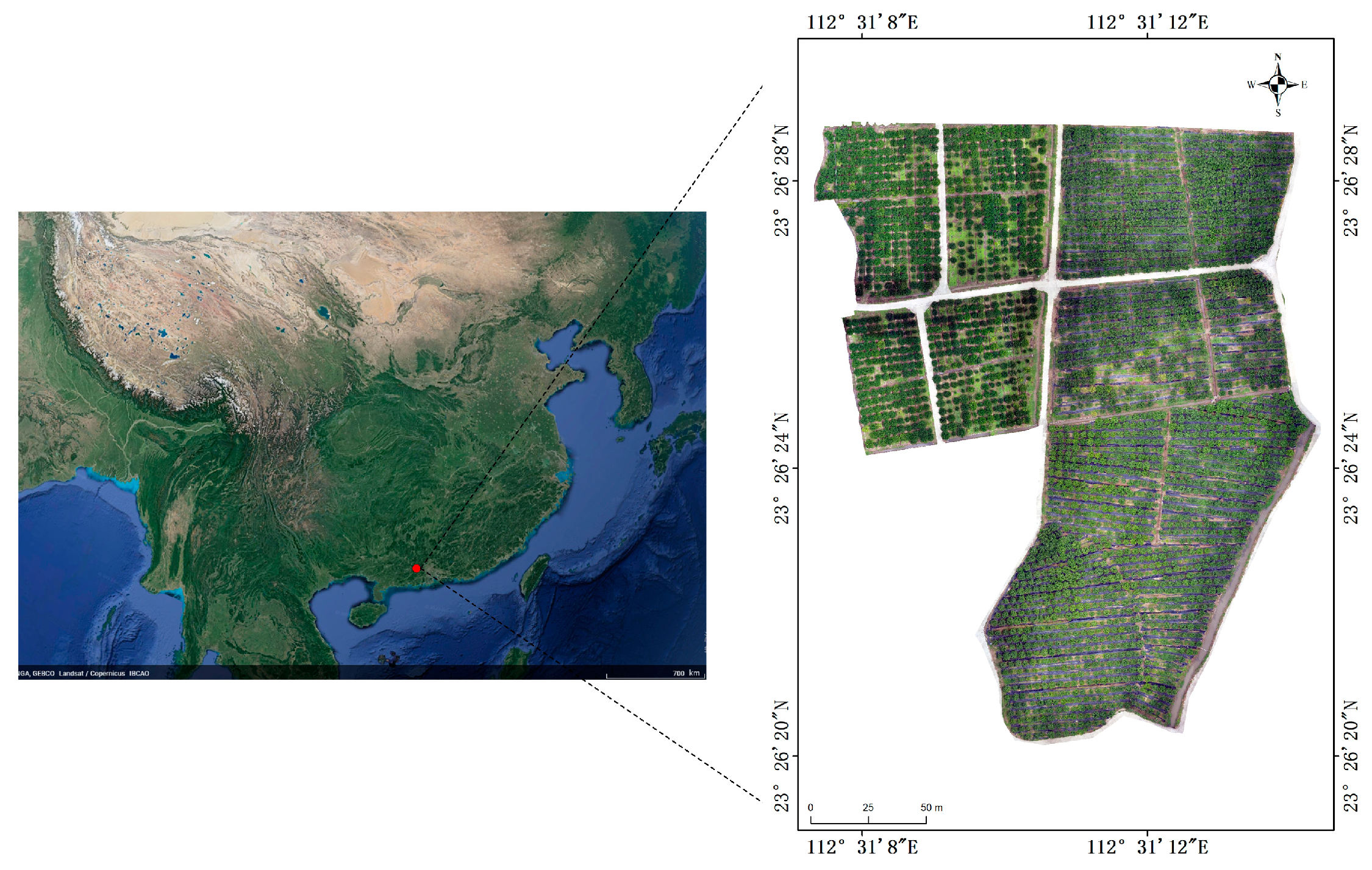
2.1.1. Research Area
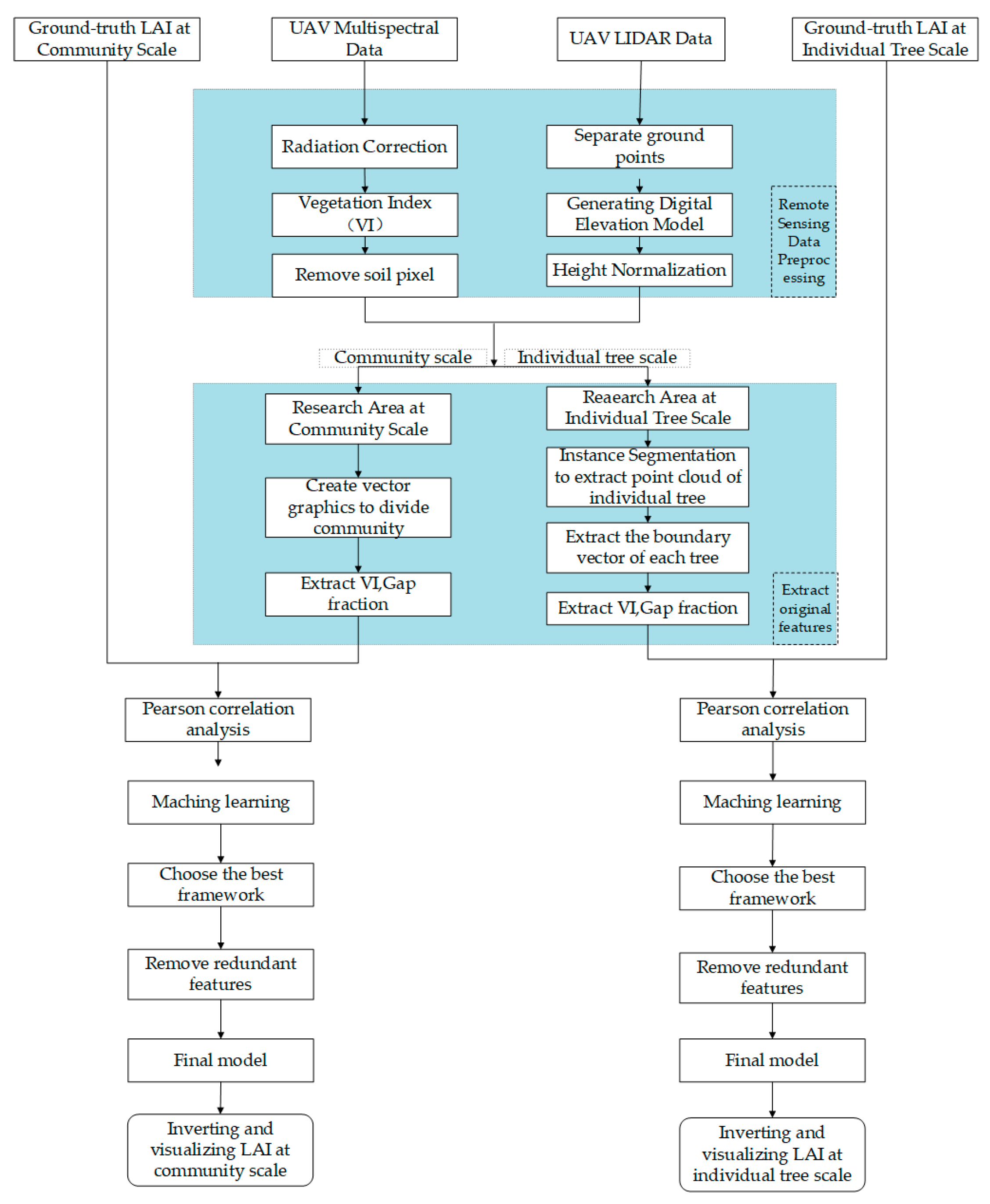
2.1.2. Technical Route
2.2. Data Acquisition
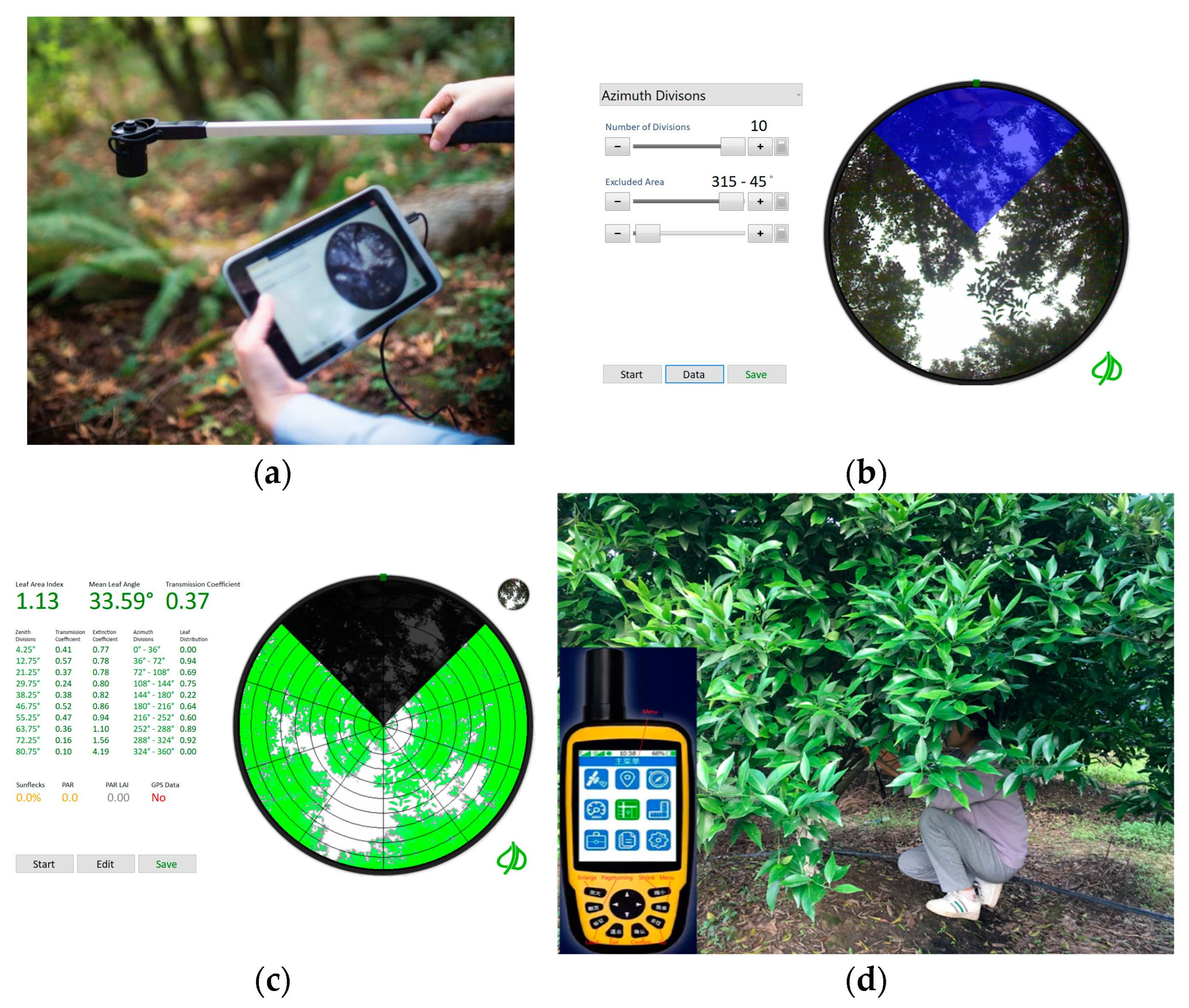
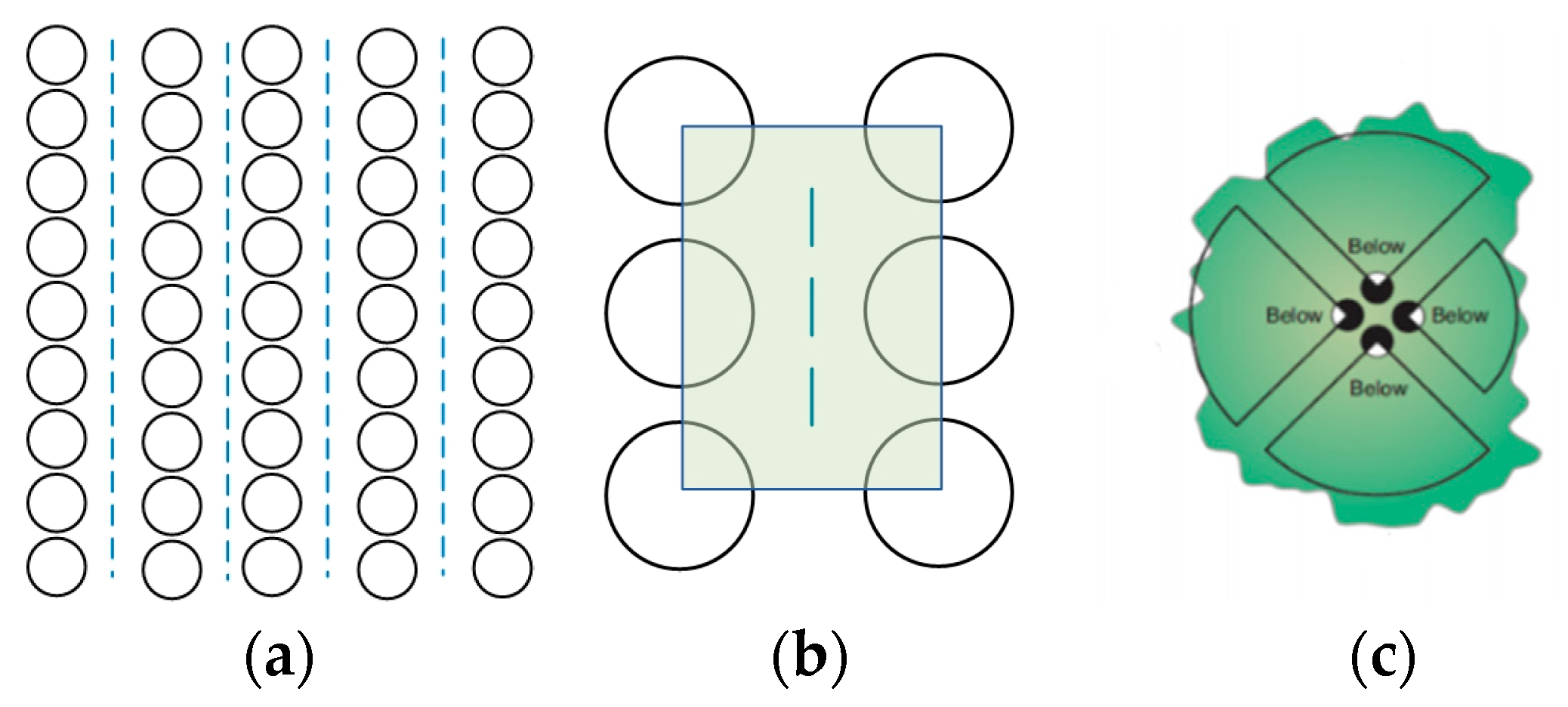
2.2.1. Ground-Truth LAI Acquisition
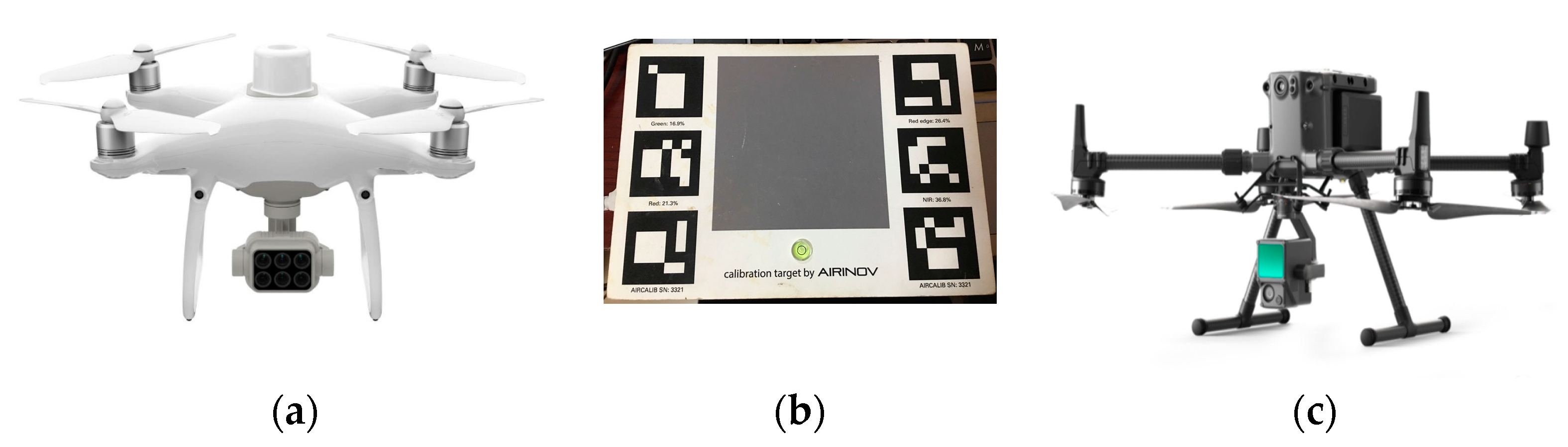
2.2.2. Remote Sensing Data Collection
2.3. Remote Sensing Data Preprocessing
2.3.1. Multispectral Data Preprocessing
Vegetation Index
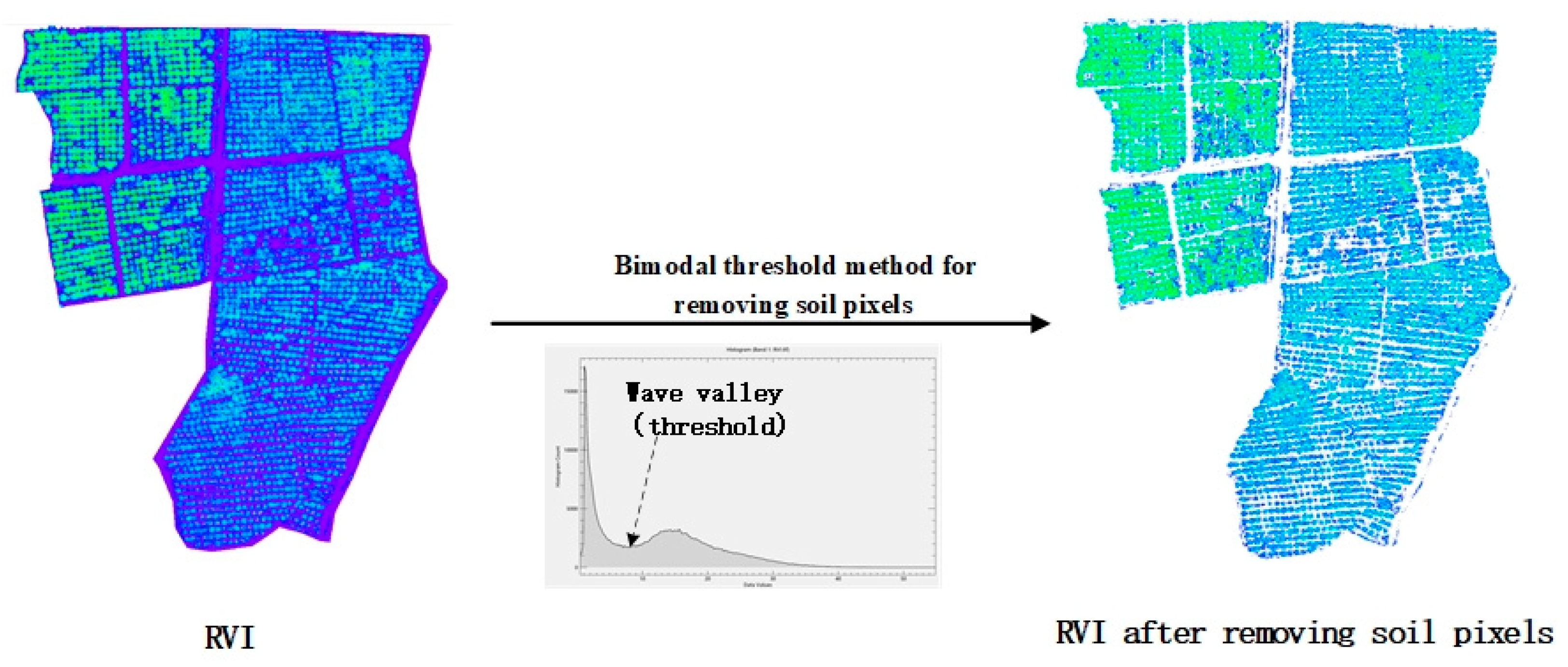
Removing Soil Background
2.3.2. LiDAR Data Preprocessing
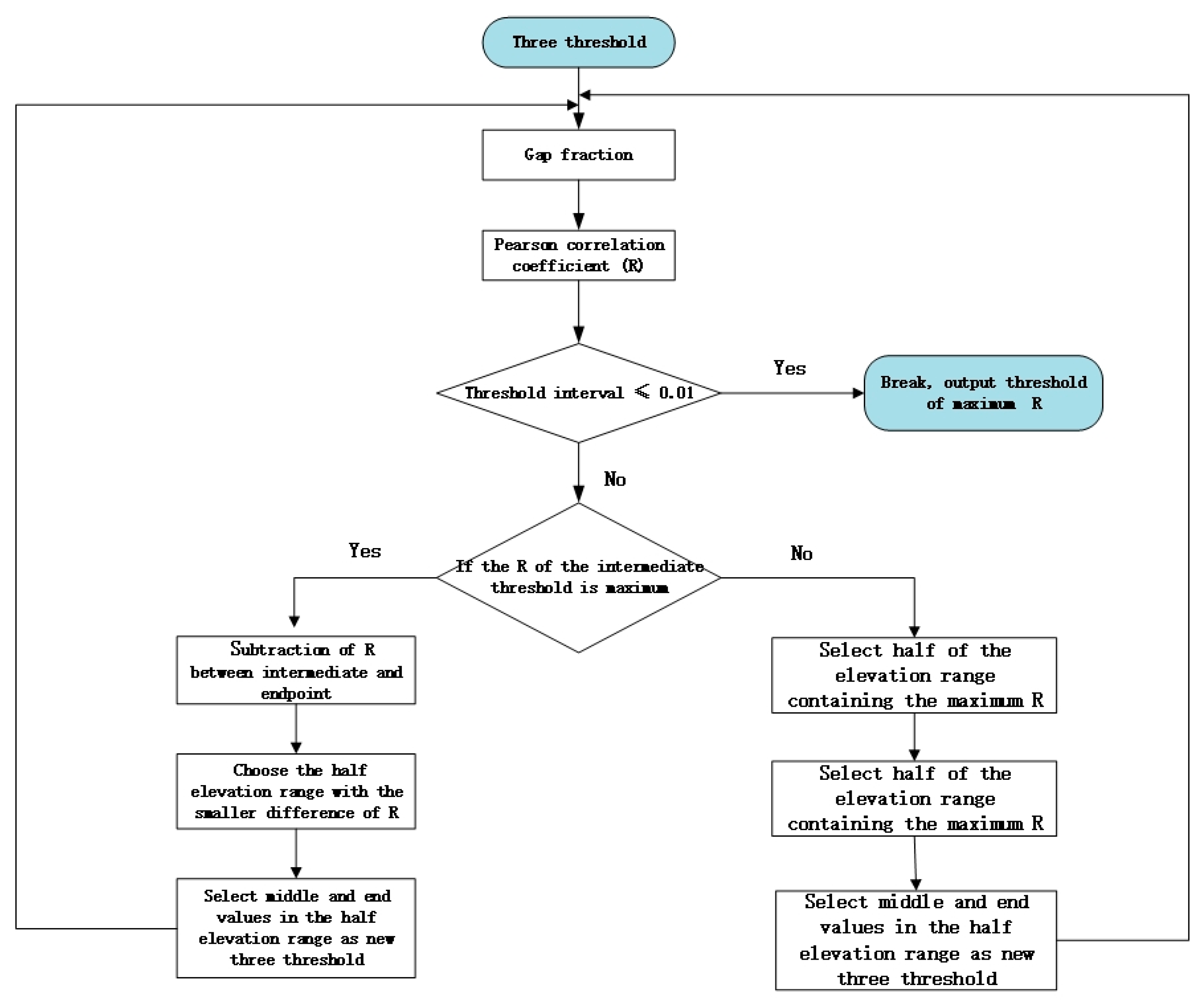
Gap Fraction
Height Normalization
2.4. Extract Features
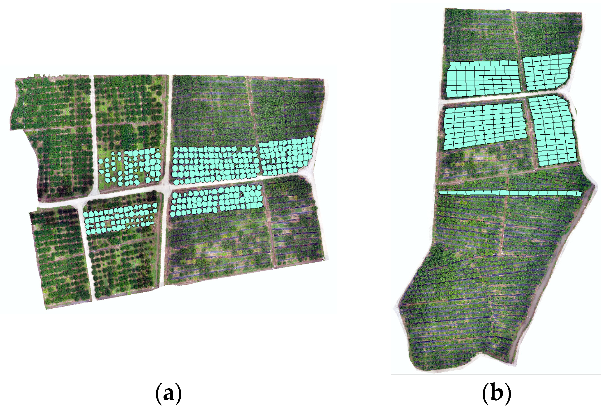
2.4.1. Community Scale
Vegetation Indices in Each ROI
Gap Fraction in Each ROI
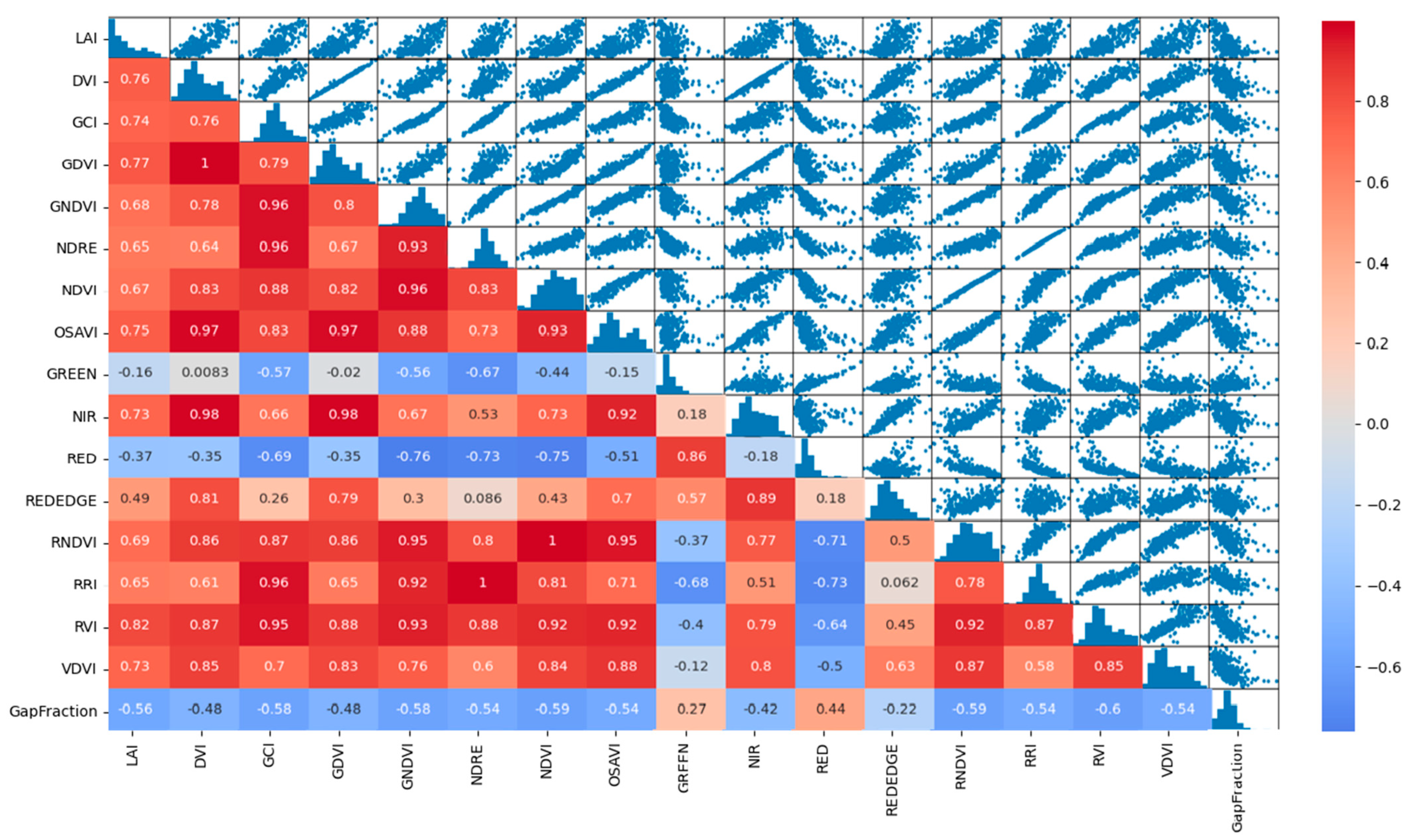
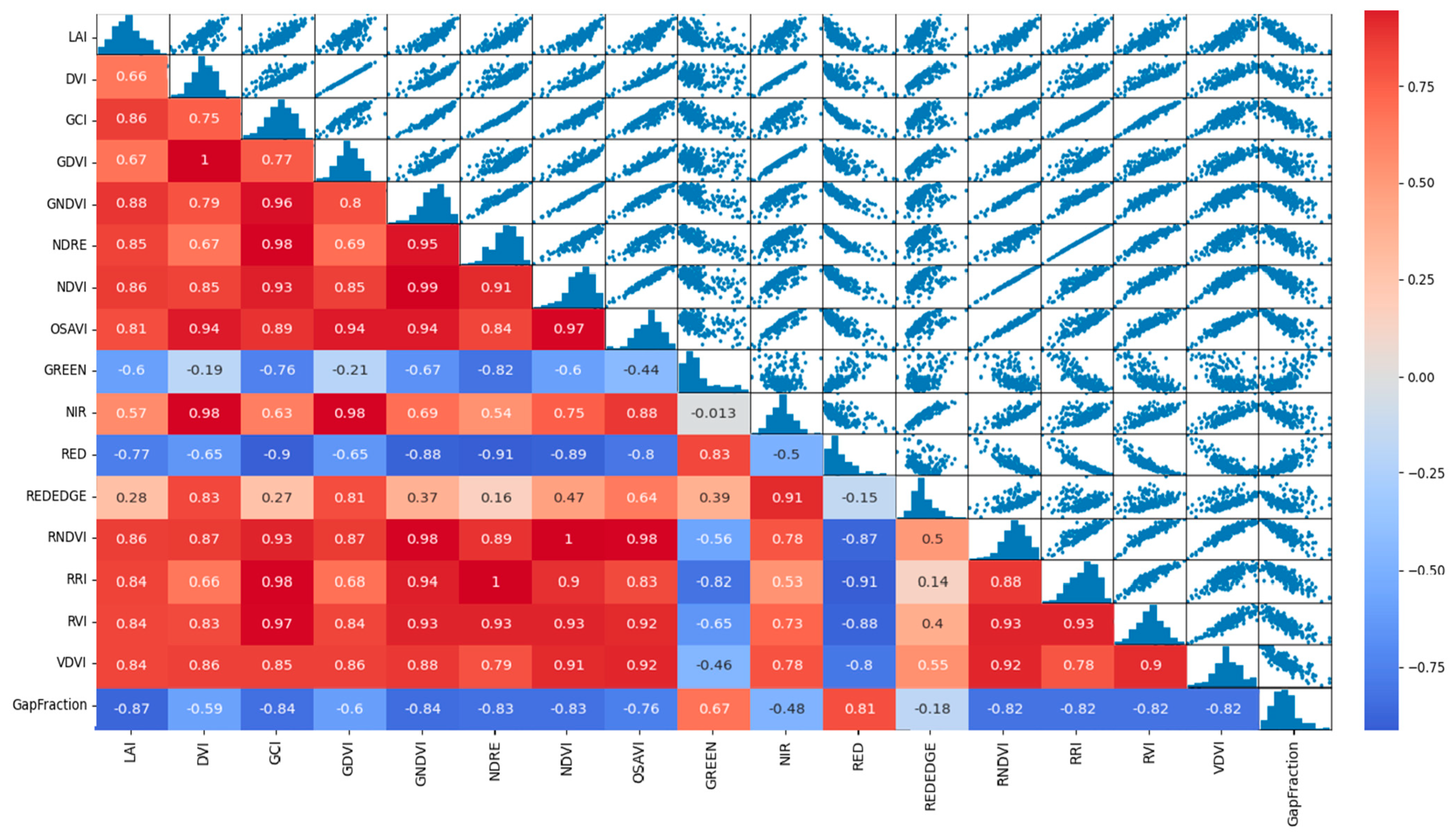
Pearson Correlation Coefficient and Scatter Plot
2.4.2. Individual Tree Scale
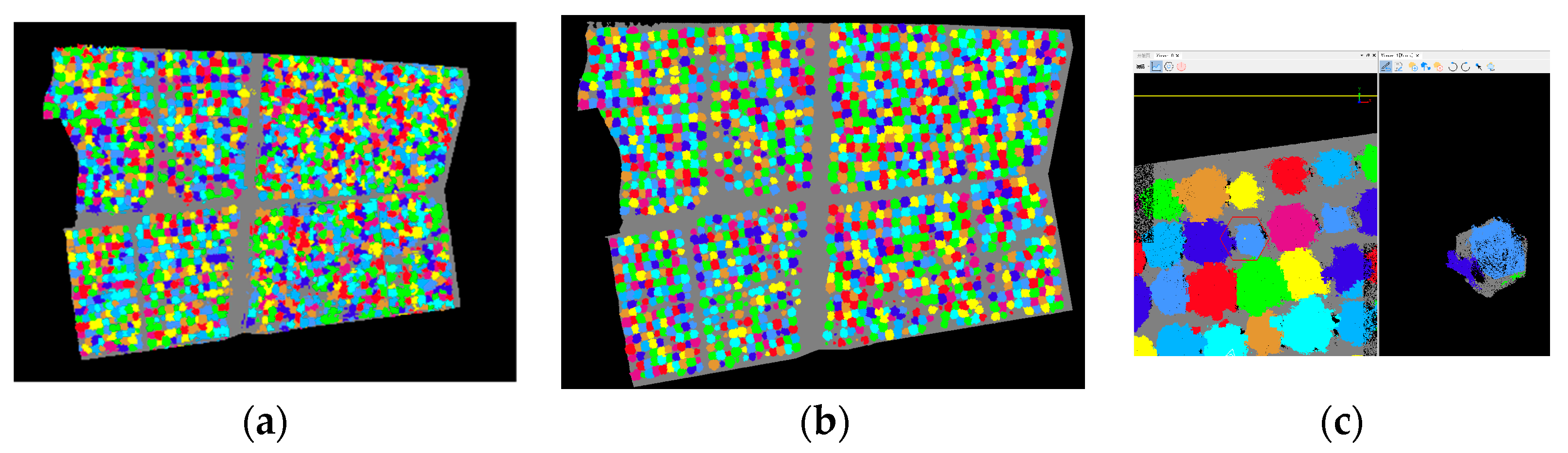
Instance Segmentation
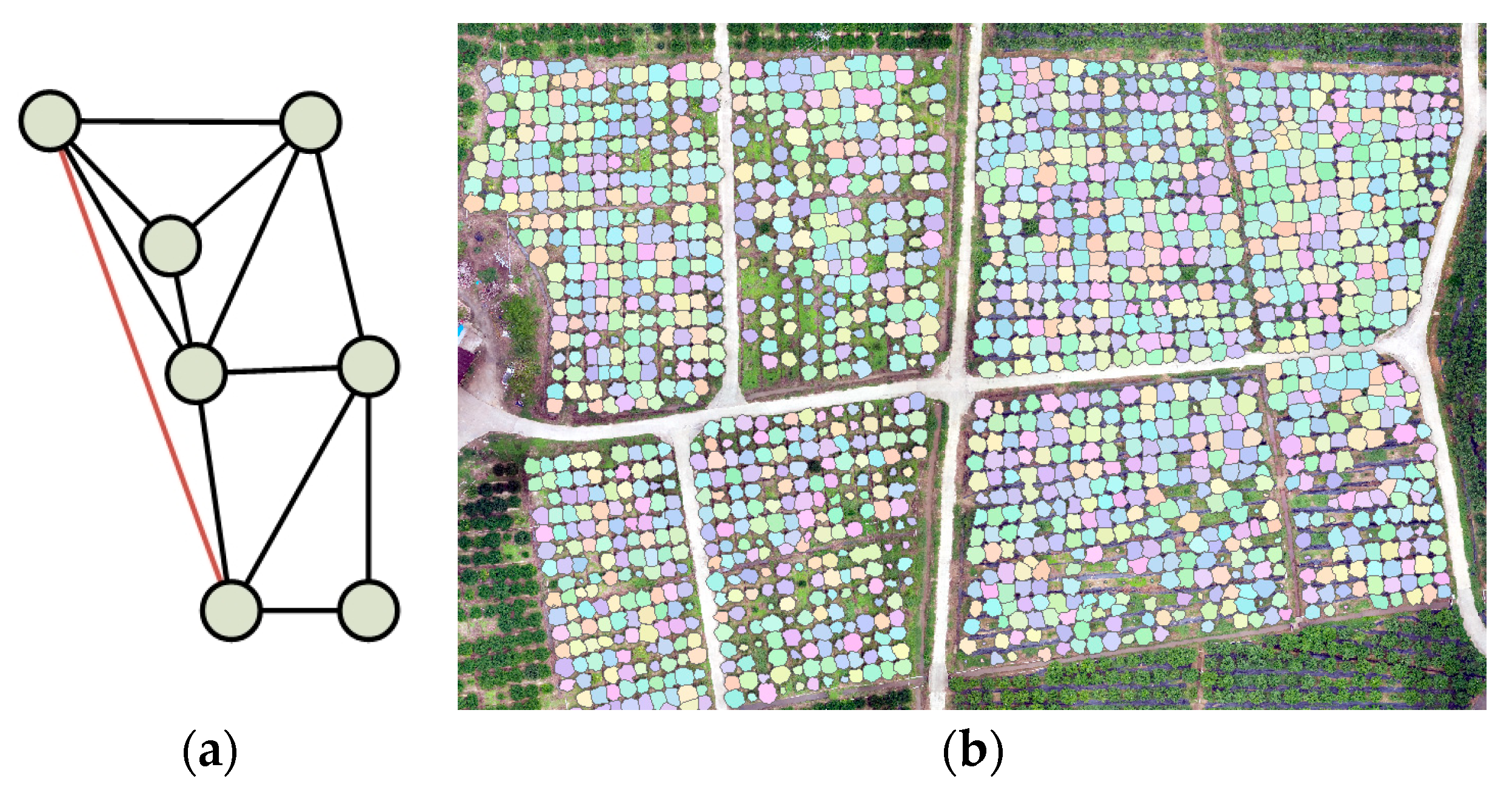
Extracting Boundary of Individual Tree
Pearson Correlation Coefficient and Scatter Plot
2.5. Regression Model
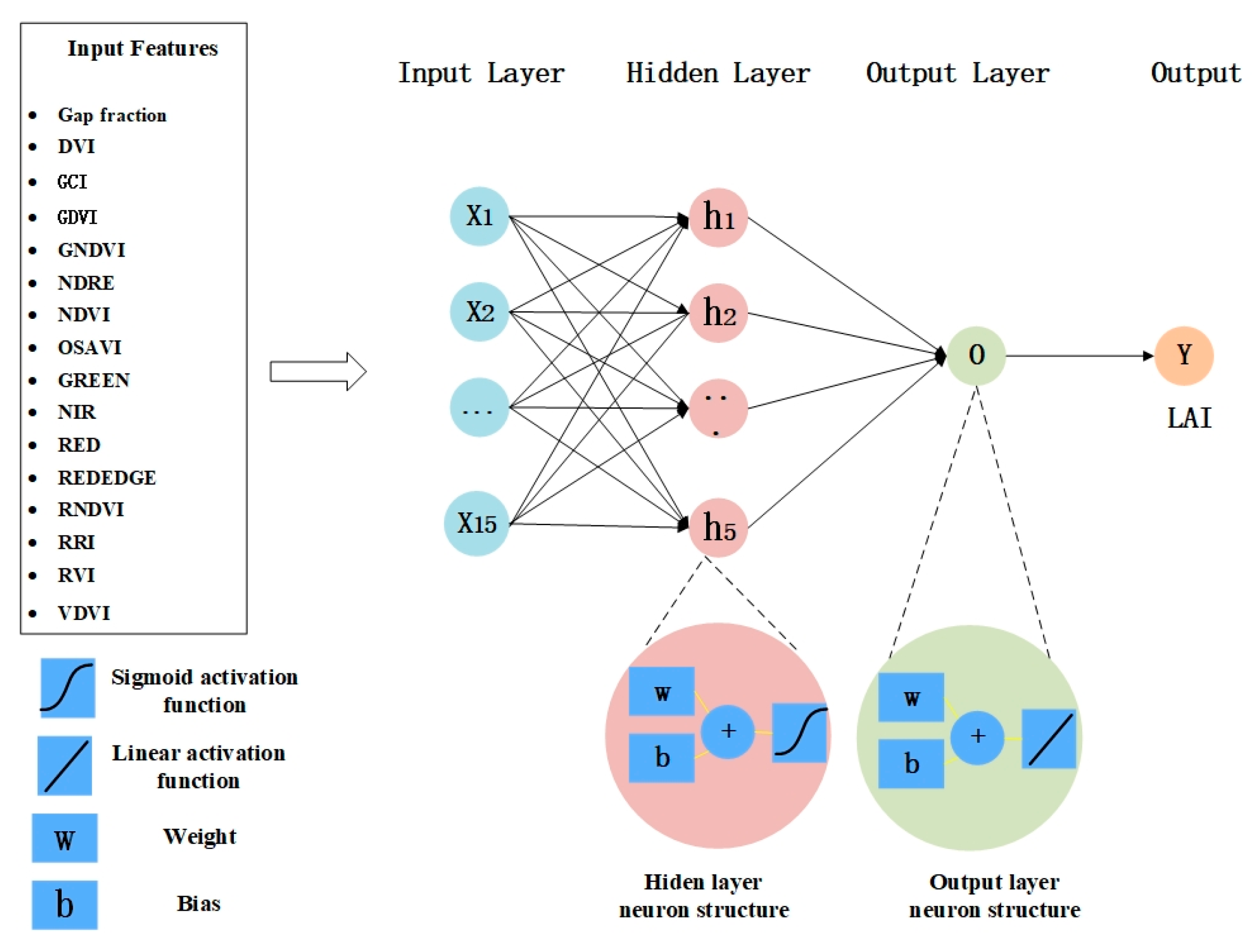
2.5.1. BP Neural Network Model
2.5.2. Other Models
3. Results
3.1. Model Comparison
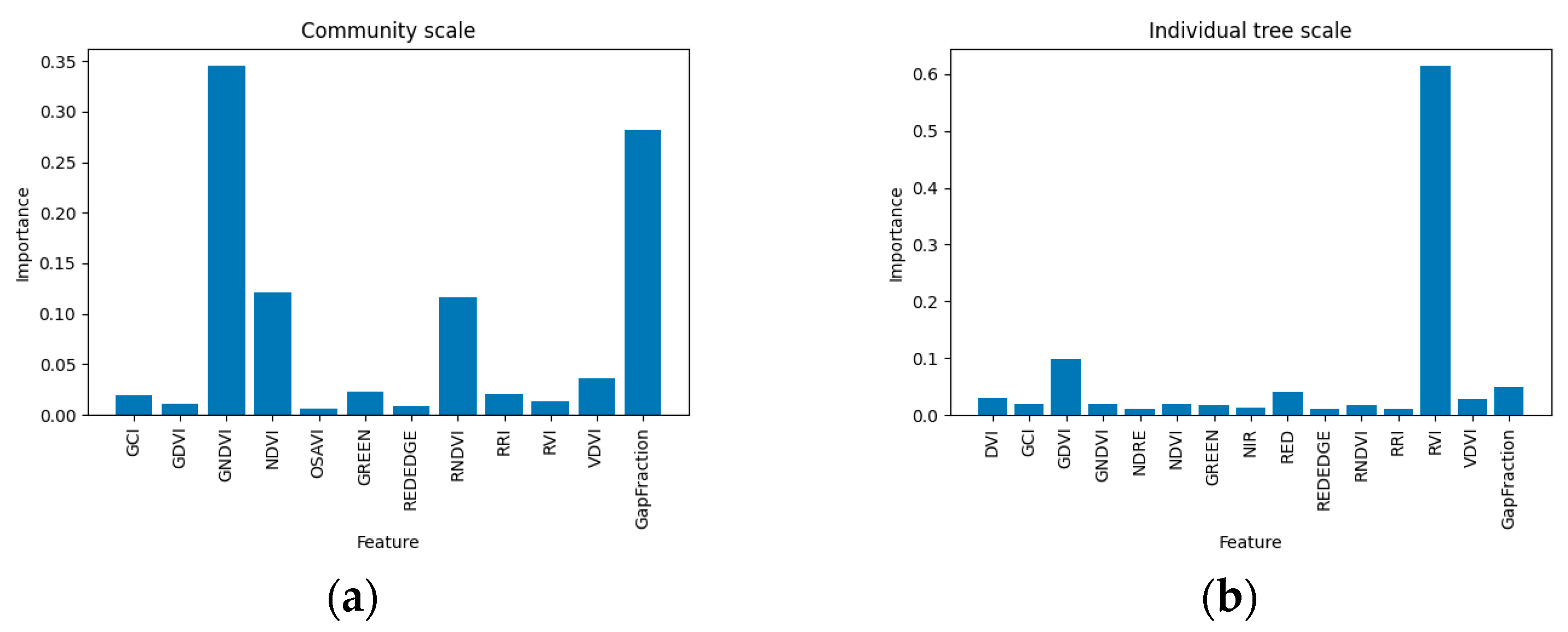
3.2. Remove Redundant Features
3.3. The Effect of Gap Fraction on Results
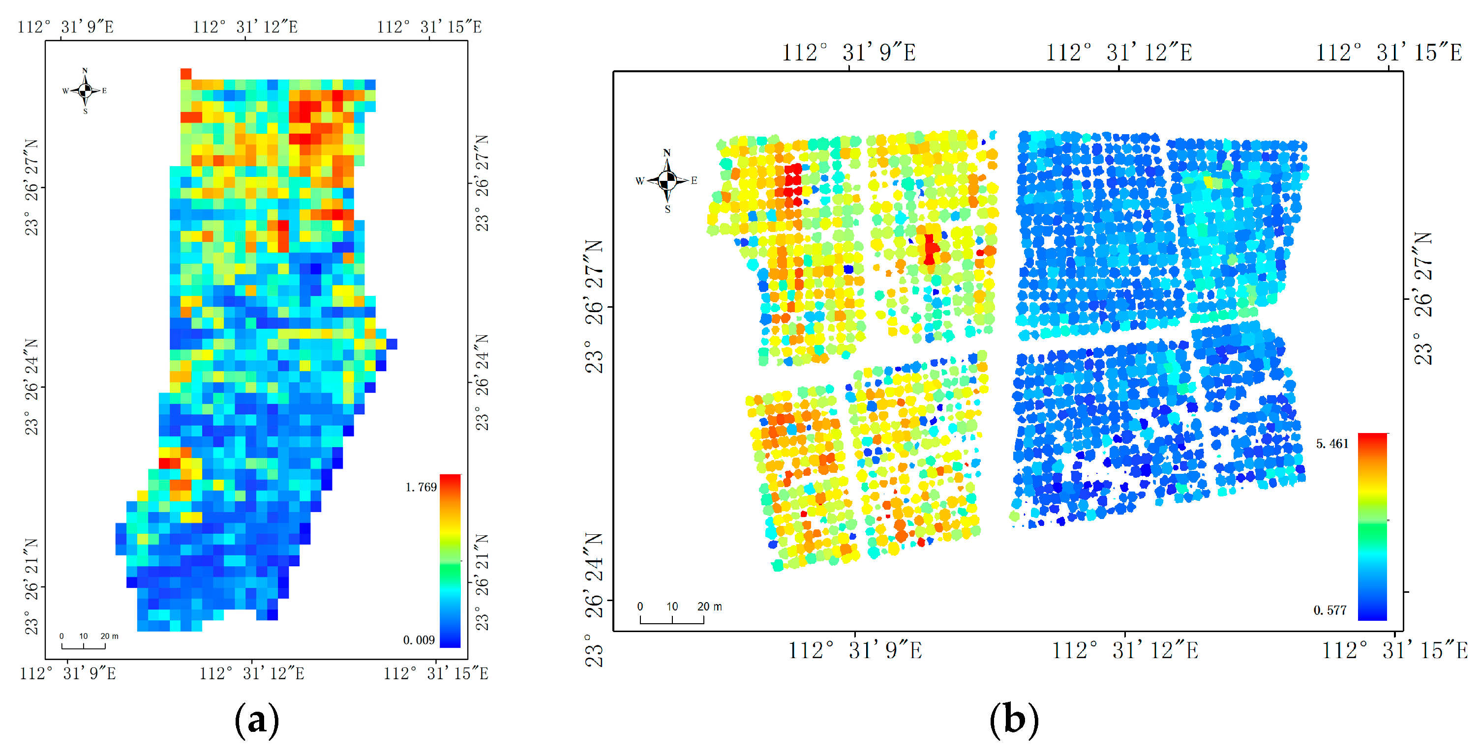
3.4. Model Application
4. Discussion
5. Conclusions
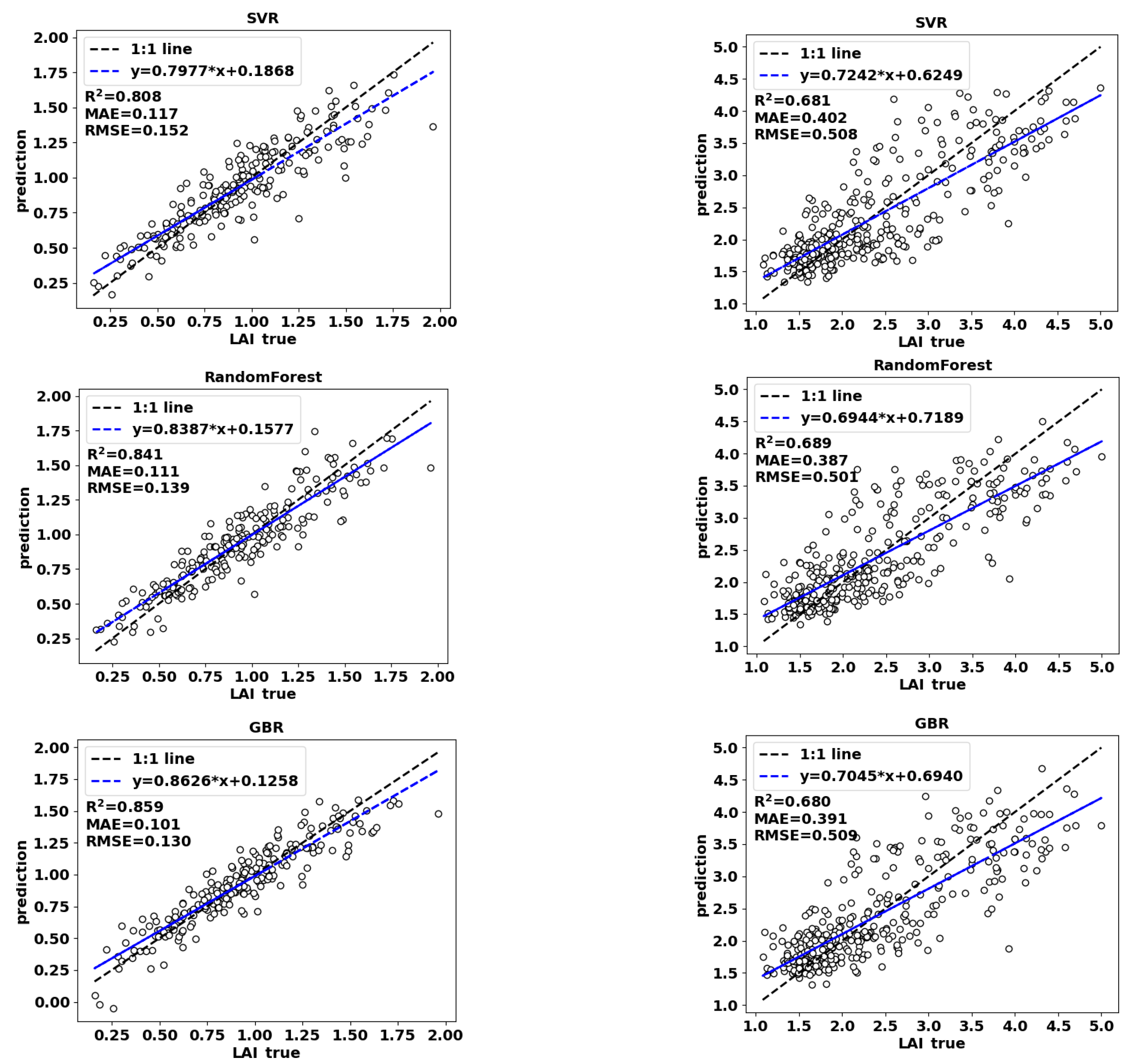
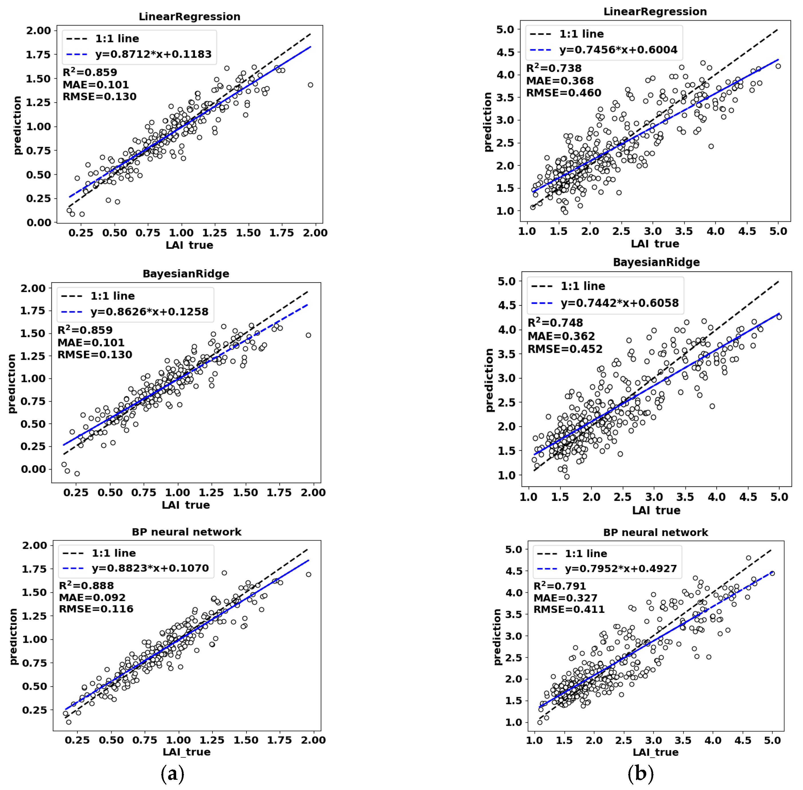
- (1)
- The R2 values of the six models at both the community scale and individual scale, before removing redundant features, were as follows: 0.808 (SVR), 0.841 (GBR), 0.859 (LR), 0.859 (RF), 0.859 (Bayesian), and 0.888 (BP) for the community scale; and 0.681 (SVR), 0.680 (GBR), 0.738 (LR), 0.689 (RF), 0.748 (Bayesian), and 0.791 (BP) for the individual scale. The BP neural network demonstrated the best performance among the models at both scales.
- (2)
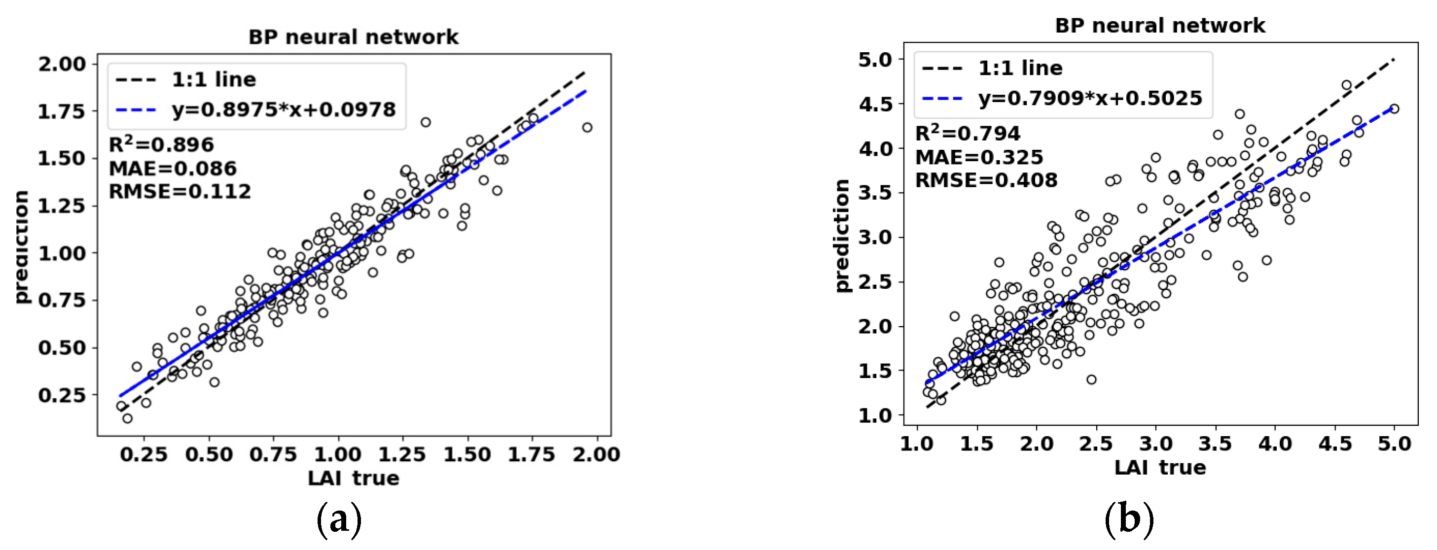
- The R2 values of the BP neural network model, after removing redundant features, were found to be 0.896 at the community scale and 0.794 at the individual scale. It was observed that the model achieved higher accuracy at the community scale compared to the individual scale.
- (3)
- By integrating LiDAR data with multispectral data, we observed a substantial improvement in the R2 values. Specifically, at the community scale, there was a notable increase of 4.43%, while at the individual scale, the improvement reached an impressive 7.29%. These results strongly suggest that the fusion approach, which combines the two-dimensional multispectral information with the three-dimensional spatial information, outperforms the conventional two-dimensional multispectral methods.
Author Contributions
Funding
Data Availability Statement
Conflicts of Interest
References
- Wang, Y.; Leuning, R. A two-leaf model for canopy conductance, photosynthesis and partitioning of available energy I.: Model description and comparison with a multi-layered model. Agric. Forest Meteorol. 1998, 91, 89–111. [Google Scholar] [CrossRef]
- Calvet, J.; Noilhan, J.; Roujean, J.; Bessemoulin, P.; Cabelguenne, M.; Olioso, A.; Wigneron, J. An interactive vegetation SVAT model tested against data from six contrasting sites. Agric. Forest Meteorol. 1998, 92, 73–95. [Google Scholar] [CrossRef]
- Asner, G.P.; Scurlock, J.M.; Hicke, J.A. Global synthesis of leaf area index observations: Implications for ecological and remote sensing studies. Glob. Ecol. Biogeogr. 2003, 12, 191–205. [Google Scholar] [CrossRef]
- Sellers, P.J.; Dickinson, R.E.; Randall, D.A.; Betts, A.K.; Hall, F.G.; Berry, J.A.; Collatz, G.J.; Denning, A.S.; Mooney, H.A.; Nobre, C.A. Modeling the exchanges of energy, water, and carbon between continents and the atmosphere. Science 1997, 275, 502–509. [Google Scholar] [CrossRef]
- Watson, D.J. Comparative physiological studies on the growth of field crops: II. The effect of varying nutrient supply on net assimilation rate and leaf area. Ann. Bot. London 1947, 11, 375–407. [Google Scholar] [CrossRef]
- Verrelst, J.; Rivera, J.P.; Veroustraete, F.; Muñoz-Marí, J.; Clevers, J.G.; Camps-Valls, G.; Moreno, J. Experimental Sentinel-2 LAI estimation using parametric, non-parametric and physical retrieval methods—A comparison. ISPRS J. Photogramm. 2015, 108, 260–272. [Google Scholar] [CrossRef]
- Zhai, C.; Zhao, C.; Ning, W.; Long, J.; Wang, X.; Weckler, P.; Zhang, H. Research progress on precision control methods of air-assisted spraying in orchards. Trans. Chin. Soc. Agric. Eng. 2018, 34, 1–15. [Google Scholar]
- Liao, J.; Zang, Y.; Luo, X.; Zhou, Z.; Zang, Y.; Wang, P.; Hewitt, A.J. The relations of leaf area index with the spray quality and efficacy of cotton defoliant spraying using unmanned aerial systems (UASs). Comput. Electron. Agric. 2020, 169, 105228. [Google Scholar] [CrossRef]
- Qi, H.; Zhu, B.; Wu, Z.; Liang, Y.; Li, J.; Wang, L.; Chen, T.; Lan, Y.; Zhang, L. Estimation of peanut leaf area index from unmanned aerial vehicle multispectral images. Sensors 2020, 20, 6732. [Google Scholar] [CrossRef]
- Bréda, N.J. Ground-based measurements of leaf area index: A review of methods, instruments and current controversies. J. Exp. Bot. 2003, 54, 2403–2417. [Google Scholar] [CrossRef]
- Zheng, G.; Moskal, L.M. Retrieving leaf area index (LAI) using remote sensing: Theories, methods and sensors. Sensors 2009, 9, 2719–2745. [Google Scholar] [CrossRef] [PubMed]
- Jonckheere, I.; Fleck, S.; Nackaerts, K.; Muys, B.; Coppin, P.; Weiss, M.; Baret, F. Review of methods for in situ leaf area index determination: Part I. Theories, sensors and hemispherical photography. Agric. Forest Meteorol. 2004, 121, 19–35. [Google Scholar] [CrossRef]
- Klingler, A.; Schaumberger, A.; Vuolo, F.; Kalmár, L.B.; Pötsch, E.M. Comparison of direct and indirect determination of leaf area index in permanent grassland. PFG—J. Photogramm. Remote Sens. Geoinf. Sci. 2020, 88, 369–378. [Google Scholar] [CrossRef]
- Schraik, D.; Varvia, P.; Korhonen, L.; Rautiainen, M. Bayesian inversion of a forest reflectance model using sentinel-2 and landsat 8 satellite images. J. Quant. Spectrosc. Radiat. Transfer. 2019, 233, 1–12. [Google Scholar] [CrossRef]
- Lee, J.; Kang, Y.; Son, B.; Im, J.; Jang, K. Estimation of Leaf Area Index Based on Machine Learning/PROSAIL Using Optical Satellite Imagery. Korean J. Remote Sens. 2021, 37, 1719–1729. [Google Scholar]
- Kang, Y.; Gao, F.; Anderson, M.; Kustas, W.; Nieto, H.; Knipper, K.; Yang, Y.; White, W.; Alfieri, J.; Torres-Rua, A. Evaluation of satellite Leaf Area Index in California vineyards for improving water use estimation. Irrig. Sci. 2022, 40, 531–551. [Google Scholar] [CrossRef]
- Weiss, M.; Jacob, F.; Duveiller, G. Remote sensing for agricultural applications: A meta-review. Remote Sens. Environ. 2020, 236, 111402. [Google Scholar] [CrossRef]
- Wang, Y.; Fang, H. Estimation of LAI with the LiDAR technology: A review. Remote Sens. 2020, 12, 3457. [Google Scholar] [CrossRef]
- Ali, A.; Imran, M. Evaluating the potential of red edge position (REP) of hyperspectral remote sensing data for real time estimation of LAI & chlorophyll content of kinnow mandarin (Citrus reticulata) fruit orchards. Sci. Hortic. 2020, 267, 109326. [Google Scholar]
- Ma, J.; Wang, L.; Chen, P. Comparing different methods for wheat LAI inversion based on hyperspectral data. Agriculture 2022, 12, 1353. [Google Scholar] [CrossRef]
- Pagliai, A.; Ammoniaci, M.; Sarri, D.; Lisci, R.; Perria, R.; Vieri, M.; D’Arcangelo, M.E.M.; Storchi, P.; Kartsiotis, S. Comparison of Aerial and Ground 3D Point Clouds for Canopy Size Assessment in Precision Viticulture. Remote Sens. 2022, 14, 1145. [Google Scholar] [CrossRef]
- Colaço, A.F.; Trevisan, R.G.; Molin, J.P.; Rosell-Polo, J.R.; Escolà, A. A method to obtain orange crop geometry information using a mobile terrestrial laser scanner and 3D modeling. Remote Sens. 2017, 9, 763. [Google Scholar] [CrossRef]
- Li, Q.; Xue, Y. Total leaf area estimation based on the total grid area measured using mobile laser scanning. Comput. Electron. Agric. 2023, 204, 107503. [Google Scholar] [CrossRef]
- Luo, S.; Chen, J.M.; Wang, C.; Gonsamo, A.; Xi, X.; Lin, Y.; Qian, M.; Peng, D.; Nie, S.; Qin, H. Comparative performances of airborne LiDAR height and intensity data for leaf area index estimation. IEEE J. Sel. Top. Appl. Earth Obs. Remote Sens. 2017, 11, 300–310. [Google Scholar] [CrossRef]
- Tang, H.; Brolly, M.; Zhao, F.; Strahler, A.H.; Schaaf, C.L.; Ganguly, S.; Zhang, G.; Dubayah, R. Deriving and validating Leaf Area Index (LAI) at multiple spatial scales through lidar remote sensing: A case study in Sierra National Forest, CA. Remote Sens. Environ. 2014, 143, 131–141. [Google Scholar] [CrossRef]
- Lang, A.; Yueqin, X. Estimation of leaf area index from transmission of direct sunlight in discontinuous canopies. Agric. Forest Meteorol. 1986, 37, 229–243. [Google Scholar] [CrossRef]
- Tunca, E.; Köksal, E.S.; Çetin, S.; Ekiz, N.M.; Balde, H. Yield and leaf area index estimations for sunflower plants using unmanned aerial vehicle images. Environ. Monit. Assess. 2018, 190, 1–12. [Google Scholar] [CrossRef]
- López-Calderón, M.J.; Estrada-Ávalos, J.; Rodríguez-Moreno, V.M.; Mauricio-Ruvalcaba, J.E.; Martínez-Sifuentes, A.R.; Delgado-Ramírez, G.; Miguel-Valle, E. Estimation of total nitrogen content in forage maize (Zea mays L.) Using Spectral Indices: Analysis by Random Forest. Agriculture 2020, 10, 451. [Google Scholar] [CrossRef]
- Shen, B.; Ding, L.; Ma, L.; Li, Z.; Pulatov, A.; Kulenbekov, Z.; Chen, J.; Mambetova, S.; Hou, L.; Xu, D. Modeling the Leaf Area Index of Inner Mongolia Grassland Based on Machine Learning Regression Algorithms Incorporating Empirical Knowledge. Remote Sens. 2022, 14, 4196. [Google Scholar] [CrossRef]
- Zhang, Z.; Masjedi, A.; Zhao, J.; Crawford, M.M. Prediction of sorghum biomass based on image based features derived from time series of UAV images. In Proceedings of the 2017 IEEE International Geoscience and Remote Sensing Symposium (IGARSS), Fort Worth, TX, USA, 23–28 July 2017; pp. 6154–6417. [Google Scholar]
- Mansaray, L.R.; Kabba, V.T.; Yang, L. Rice biophysical parameter retrieval with optical satellite imagery: A comparative assessment of parametric and non-parametric models. Geocarto Int. 2022, 37, 13561–13578. [Google Scholar] [CrossRef]
- Zhu, X.; Li, J.; Liu, Q.; Yu, W.; Li, S.; Zhao, J.; Dong, Y.; Zhang, Z.; Zhang, H.; Lin, S. Use of a BP Neural Network and Meteorological Data for Generating Spatiotemporally Continuous LAI Time Series. IEEE Trans. Geosci. Remote Sens. 2021, 60, 1–14. [Google Scholar] [CrossRef]
- Li, S.; Yuan, F.; Ata-UI-Karim, S.T.; Zheng, H.; Cheng, T.; Liu, X.; Tian, Y.; Zhu, Y.; Cao, W.; Cao, Q. Combining color indices and textures of UAV-based digital imagery for rice LAI estimation. Remote Sens. 2019, 11, 1763. [Google Scholar] [CrossRef]
- Yan, P.; Han, Q.; Feng, Y.; Kang, S. Estimating lai for cotton using multisource uav data and a modified universal model. Remote Sens. 2022, 14, 4272. [Google Scholar] [CrossRef]
- Hasan, U.; Sawut, M.; Chen, S. Estimating the leaf area index of winter wheat based on unmanned aerial vehicle RGB-image parameters. Sustainability 2019, 11, 6829. [Google Scholar] [CrossRef]
- Sun, X.; Yang, Z.; Su, P.; Wei, K.; Wang, Z.; Yang, C.; Wang, C.; Qin, M.; Xiao, L.; Yang, W. Non-destructive monitoring of maize LAI by fusing UAV spectral and textural features. Front. Plant Sci. 2023, 14, 1158837. [Google Scholar] [CrossRef] [PubMed]
- Černý, J.; Pokorný, R.; Haninec, P.; Bednář, P. Leaf area index estimation using three distinct methods in pure deciduous stands. J. Vis. Exp. 2019, 150, e59757. [Google Scholar]
- Zhang, X.; Zhang, K.; Wu, S.; Shi, H.; Sun, Y.; Zhao, Y.; Fu, E.; Chen, S.; Bian, C.; Ban, W. An investigation of winter wheat leaf area index fitting model using spectral and canopy height model data from unmanned aerial vehicle imagery. Remote Sens. 2022, 14, 5087. [Google Scholar] [CrossRef]
- Gitelson, A.A.; Merzlyak, M.N. Remote sensing of chlorophyll concentration in higher plant leaves. Adv. Space Res. 1998, 22, 689–692. [Google Scholar] [CrossRef]
- Peñuelas, J.; Isla, R.; Filella, I.; Araus, J.L. Visible and near-infrared reflectance assessment of salinity effects on barley. Crop Sci. 1997, 37, 198–202. [Google Scholar] [CrossRef]
- Gitelson, A.; Merzlyak, M.N. Spectral reflectance changes associated with autumn senescence of Aesculus hippocastanum L. and Acer platanoides L. leaves. Spectral features and relation to chlorophyll estimation. J. Plant Physiol. 1994, 143, 286–292. [Google Scholar] [CrossRef]
- Rondeaux, G.; Steven, M.; Baret, F. Optimization of soil-adjusted vegetation indices. Remote Sens. Environ. 1996, 55, 95–107. [Google Scholar] [CrossRef]
- Jordan, C.F. Derivation of leaf-area index from quality of light on the forest floor. Ecology 1969, 50, 663–666. [Google Scholar] [CrossRef]
- Wu, W. The generalized difference vegetation index (GDVI) for dryland characterization. Remote Sens. 2014, 6, 1211–1233. [Google Scholar] [CrossRef]
- Becker, F.; Choudhury, B.J. Relative sensitivity of normalized difference vegetation index (NDVI) and microwave polarization difference index (MDPI) for vegetation and desertification monitoring. Remote Sens. Environ. 1988, 24, 297–311. [Google Scholar] [CrossRef]
- Xiao, H.; Chen, X.; Yang, Z.; Li, H.; Zhu, H. Vegetation index estimation by chlorophyll content of grassland based on spectral analysis. Spectrosc. Spect. Anal. 2014, 34, 3075–3078. [Google Scholar]
- Cao, Q.; Miao, Y.; Gao, X.; Liu, B.; Feng, G.; Yue, S. Estimating the nitrogen nutrition index of winter wheat using an active canopy sensor in the North China Plain. In Proceedings of the 2012 First International Conference on Agro-Geoinformatics (Agro-Geoinformatics), Shanghai, China, 2–4 August 2012; pp. 1–5. [Google Scholar]
- Xiaoqin, W.; Miaomiao, W.; Shaoqiang, W.; Yundong, W. Extraction of vegetation information from visible unmanned aerial vehicle images. Trans. Chin. Soc. Agric. Eng. 2015, 31, 152–159. [Google Scholar]
- Wu, H.; Jiang, J.J.; Zhang, H.L.; Zhang, L.; Zhou, J. Application of ratio resident-area index to retrieve urban residential areas based on landsat TM data. J. Nanjing Norm. Univ. Nat. Sci. 2006, 3, 118–121. [Google Scholar]
- Zhao, X.; Guo, Q.; Su, Y.; Xue, B. Improved progressive TIN densification filtering algorithm for airborne LiDAR data in forested areas. ISPRS J. Photogramm. 2016, 117, 79–91. [Google Scholar] [CrossRef]
- Chen, Q.; Baldocchi, D.; Gong, P.; Kelly, M. Isolating individual trees in a savanna woodland using small footprint lidar data. Photogramm. Eng. Remote Sens. 2006, 72, 923–932. [Google Scholar] [CrossRef]
- Ma, K.; Chen, Z.; Fu, L.; Tian, W.; Jiang, F.; Yi, J.; Du, Z.; Sun, H. Performance and sensitivity of individual tree segmentation methods for UAV-LiDAR in multiple forest types. Remote Sens. 2022, 14, 298. [Google Scholar] [CrossRef]
- Rumelhart, D.E.; Hinton, G.E.; Williams, R.J. Learning representations by back-propagating errors. Nature 1986, 323, 533–536. [Google Scholar] [CrossRef]
- Rigatti, S.J. Random forest. J. Insur. Med. 2017, 47, 31–39. [Google Scholar] [CrossRef] [PubMed]
- Friedman, J.H. Greedy function approximation: A gradient boosting machine. Ann. Stat. 2001, 29, 1189–1232. [Google Scholar] [CrossRef]
- Awad, M.; Khanna, R.; Awad, M.; Khanna, R. Support vector regression. In Efficient Learning Machines: Theories, Concepts, and Applications for Engineers and System Designers; Springer Nature: New York, NY, USA, 2015; pp. 67–80. [Google Scholar]
- Su, X.; Yan, X.; Tsai, C.L. Linear regression. Wiley Interdiscip. Rev. Comput. Stat. 2012, 4, 275–294. [Google Scholar] [CrossRef]
- Shi, Q.; Abdel-Aty, M.; Lee, J. A Bayesian ridge regression analysis of congestion’s impact on urban expressway safety. Accid. Anal. Prev. 2016, 88, 124–137. [Google Scholar] [CrossRef] [PubMed]
- Di Gennaro, S.F.; Matese, A. Evaluation of novel precision viticulture tool for canopy biomass estimation and missing plant detection based on 2.5D and 3D approaches using RGB images acquired by UAV platform. Plant Methods 2020, 16, 1–12. [Google Scholar] [CrossRef]
- Ouyang, J.; De Bei, R.; Collins, C. Assessment of canopy size using UAV-based point cloud analysis to detect the severity and spatial distribution of canopy decline. Oeno One 2021, 55, 253–266. [Google Scholar] [CrossRef]
- López-Granados, F.; Torres-Sánchez, J.; Jiménez-Brenes, F.M.; Oneka, O.; Marín, D.; Loidi, M.; de Castro, A.I.; Santesteban, L.G. Monitoring vineyard canopy management operations using UAV-acquired photogrammetric point clouds. Remote Sens. 2020, 12, 2331. [Google Scholar] [CrossRef]
- Liu, Z.; Guo, P.; Liu, H.; Fan, P.; Zeng, P.; Liu, X.; Feng, C.; Wang, W.; Yang, F. Gradient boosting estimation of the leaf area index of apple orchards in uav remote sensing. Remote Sens. 2021, 13, 3263. [Google Scholar] [CrossRef]
- Yao, X.; Wang, N.; Liu, Y.; Cheng, T.; Tian, Y.; Chen, Q.; Zhu, Y. Estimation of wheat LAI at middle to high levels using unmanned aerial vehicle narrowband multispectral imagery. Remote Sens. 2017, 9, 1304. [Google Scholar] [CrossRef]
- He, L.; Ren, X.; Wang, Y.; Liu, B.; Zhang, H.; Liu, W.; Feng, W.; Guo, T. Comparing methods for estimating leaf area index by multi-angular remote sensing in winter wheat. Sci. Rep. 2020, 10, 13943. [Google Scholar] [CrossRef] [PubMed]


| Scale | Number of Samples | Max | Min | Mean | Standard Deviation |
|---|---|---|---|---|---|
| Community | 220 | 1.963 | 0.160 | 0.927 | 0.348 |
| Individual | 341 | 5.00 | 1.080 | 2.372 | 0.901 |
| Parameter Name | Value |
|---|---|
| CMOS pixel | 1600 × 1300 |
| Flight altitude | 35 m |
| Course overlap | 75% |
| Lateral overlap | 75% |
| Speed of flight | 3 m/s |
| Photography mode | Equidistant photography |
| Pan tilt angle | −90° |
| Band | Blue (450 nm ± 16 nm) Green (560 nm ± 16 nm) Red (650 nm ± 16 nm) Red edge (730 nm ± 16 nm) Near infrared (840 nm ± 26 nm) |
| Parameter Name | Value |
|---|---|
| Point cloud density | 4041 points/m2 |
| Flight altitude | 35 m |
| Scan mode | Repeat scan |
| Lateral overlap | 20% |
| Speed of flight | 1 m/s |
| Vegetation Index | Full Name | Formula | Reference |
|---|---|---|---|
| GNDVI | Green Normalized Difference Vegetation Index | [39] | |
| NDVI | Normalized Difference Vegetation Index | [40] | |
| NDRE | Normalized Difference Red Edge | [41] | |
| OSAVI | Optimized Soil Adjusted Vegetation Index | [42] | |
| RVI | Ratio Vegetation Index | [43] | |
| GDVI | Green Difference Vegetation Index | [44] | |
| DVI | Difference Vegetation Index | [45] | |
| GCI | Green Chlorophyll Index | − 1 | [46] |
| RNDVI | Red Normalized Difference Vegetation Index | [47] | |
| VDVI | Visible Difference Vegetation Index | [48] | |
| RRI | Red Ratio Index | [49] |
| 921 | 330 | 468 | 0.736 | 0.663 | 0.698 |
| Feature Removed | R2 (Community Scale) | R2 (Individual Tree Scale) | Whether Redundant (Community Scale, Individual Scale) |
|---|---|---|---|
| Gap fraction | 0.855 | 0.738 | ×, × |
| DVI | 0.890 | 0.780 | √, × |
| GCI | 0.886 | 0.765 | ×, × |
| GDVI | 0.883 | 0.764 | ×, × |
| GNDVI | 0.877 | 0.757 | ×, × |
| NDRE | 0.889 | 0.785 | √, × |
| NDVI | 0.872 | 0.770 | ×, × |
| OSAVI | 0.885 | 0.794 | ×, √ |
| GREEN | 0.879 | 0.789 | ×, × |
| NIR | 0.889 | 0.788 | √, × |
| RED | 0.892 | 0.784 | √, × |
| REDEDGE | 0.882 | 0.751 | ×, × |
| RNDVI | 0.887 | 0.778 | ×, × |
| RRI | 0.882 | 0.789 | ×, × |
| RVI | 0.882 | 0.758 | ×, × |
| VDVI | 0.879 | 0.784 | ×, × |
Disclaimer/Publisher’s Note: The statements, opinions and data contained in all publications are solely those of the individual author(s) and contributor(s) and not of MDPI and/or the editor(s). MDPI and/or the editor(s) disclaim responsibility for any injury to people or property resulting from any ideas, methods, instructions or products referred to in the content. |
© 2023 by the authors. Licensee MDPI, Basel, Switzerland. This article is an open access article distributed under the terms and conditions of the Creative Commons Attribution (CC BY) license (https://creativecommons.org/licenses/by/4.0/).
Share and Cite
Xu, W.; Yang, F.; Ma, G.; Wu, J.; Wu, J.; Lan, Y. Multiscale Inversion of Leaf Area Index in Citrus Tree by Merging UAV LiDAR with Multispectral Remote Sensing Data. Agronomy 2023, 13, 2747. https://doi.org/10.3390/agronomy13112747
Xu W, Yang F, Ma G, Wu J, Wu J, Lan Y. Multiscale Inversion of Leaf Area Index in Citrus Tree by Merging UAV LiDAR with Multispectral Remote Sensing Data. Agronomy. 2023; 13(11):2747. https://doi.org/10.3390/agronomy13112747
Chicago/Turabian StyleXu, Weicheng, Feifan Yang, Guangchao Ma, Jinhao Wu, Jiapei Wu, and Yubin Lan. 2023. "Multiscale Inversion of Leaf Area Index in Citrus Tree by Merging UAV LiDAR with Multispectral Remote Sensing Data" Agronomy 13, no. 11: 2747. https://doi.org/10.3390/agronomy13112747
APA StyleXu, W., Yang, F., Ma, G., Wu, J., Wu, J., & Lan, Y. (2023). Multiscale Inversion of Leaf Area Index in Citrus Tree by Merging UAV LiDAR with Multispectral Remote Sensing Data. Agronomy, 13(11), 2747. https://doi.org/10.3390/agronomy13112747