Article

Evaluation of Coffee Plants Transplanted to an Area with Surface and Deep Liming Based on Multispectral Indices Acquired Using Unmanned Aerial Vehicles

by
Rafael Alexandre Pena Barata
1,
Gabriel Araújo e Silva Ferraz
1,*,
Nicole Lopes Bento
1,
Daniel Veiga Soares
1,
Lucas Santos Santana
1,
Diego Bedin Marin
2,
Drucylla Guerra Mattos
3,
Felipe Schwerz
1,
Giuseppe Rossi
4,
Leonardo Conti
4 and
Gianluca Bambi
4
1
Agricultural Engineering Department, Federal University of Lavras, Lavras 37203-202, Brazil
2
Agricultural Research Company of Minas Gerais (EPAMIG), Viçosa 36571-000, Brazil
3
Agricultural Department, Federal University of Lavras, Lavras 37203-202, Brazil
4
Department of Agriculture, Food, Environment and Forestry, University of Florence, 50145 Florence, Italy
*
Author to whom correspondence should be addressed.
Agronomy 2023, 13(10), 2623; https://doi.org/10.3390/agronomy13102623
Submission received: 5 September 2023 / Revised: 9 October 2023 / Accepted: 12 October 2023 / Published: 17 October 2023
(This article belongs to the Special Issue New Trends in Agricultural UAV Application)

Abstract

:
The use of new technologies to monitor and evaluate the management of coffee crops allowed for a significant increase in productivity. Precision coffee farming has leveraged the development of this commodity by using remote sensing and Unmanned Aerial Vehicles (UAVs). However, the success of coffee farming in the country also resulted from management practices, including liming management in the soils. This study aimed to evaluate the response of coffee seedlings transplanted to areas subjected to deep liming in comparison to conventional (surface) liming, using vegetation indices (VIs) generated by multispectral images acquired using UAVs. The study area was overflown bimonthly by UAVs to measure the plant height, crown diameter, and chlorophyll content in the field. The VIs were generated and compared with the data measured in the field using linear time graphs and a correlation analysis. Linear regression was performed to predict the biophysical parameters as a function of the VIs. A significant difference was found only in the chlorophyll content. Most indices were correlated with the biophysical parameters, particularly the green chlorophyll index (GCI) and the canopy area calculated via vectorization. Therefore, UAVs proved to be effective coffee monitoring tools and can be recommended for coffee producers.

1. Introduction

The coffee crop has a great impact on the general scope of Brazilian exportation and has a great influence on the national agricultural chain. Despite recent advances in agriculture, the rate of increase in the crop yield has slowed down so that progress in specific areas has become insufficient to meet the challenges of the increasing demands for food, energy, and environmental resources. In this context, applications from different areas must be integrated into a multidisciplinary approach to obtain the most appropriate solutions to meet ecological and economic needs for coffee crop management [1,2]. Considering this, the generation of information through the use of images obtained with Unmanned Aerial Vehicles has become a fundamental tool in the monitoring and evaluation of coffee crops. In this context, precision coffee farming, defined in [3] as a set of techniques and technologies that help coffee growers manage their crops by considering the spatial soil parameters and individual plant characteristics, has been crucial. In addition, constant management practices and the farmers’ knowledge over the years have been essential for the success of coffee farming in the country.
In farming management, liming is a highly important soil preparation practice for coffee growing. Limestone contains calcium and magnesium. The former plays a key role in deepening the root system and increasing plant sustainability and resistance to drought, in addition to helping leaf retention, fruit ripening, and budding. The latter is a chlorophyll component and is therefore necessary for photosynthesis. Thus, a deficiency in these nutrients may compromise plant development and even lead to plant death [4,5,6].
In addition to providing nutrients, liming can increase the cation exchange capacity (CTC) and the soil pH, thereby neutralizing its acidity, which is a recurring problem in most Brazilian soils. However, calcium has limited mobility in soils. Consequently, the effect of conventional liming is restricted to the topsoil layer, that is, from 0 to 20 cm. For this reason, the root system only benefits from liming in this depth range [7,8]. Several studies have tested gypsum as an alternative to neutralize aluminum and transport calcium to deeper soil layers [9], but gypsum consists of a neutral salt and therefore is not a soil corrective [10]. Furthermore, the presence of sulfate ions may leach nutrients and the bases Ca2+, Mg2+, and K+, rendering them inaccessible to the roots [9,11]. Accordingly, liming deeper soil layers may be a good alternative to correct the soil pH and, consequently, increase the CTC and nutrient availability along the root system of the coffee tree, in addition to neutralizing the aluminum content.
Studies have assessed different liming depths for crops such as corn [12,13], sugarcane [14], and olive trees [15], generally finding good results for both soil pH correction and aluminum neutralization, or even for physical attributes of the soil. However, little research has been conducted on coffee growing at greater depths.
In recent years, remote sensing has been widely used in monitoring crops and decision making for better management practices. Spectral remote sensing allows for the early, efficient, objective, and non-destructive assessment of plant responses to environmental stress factors [16]. Plants react to biotic and abiotic stresses through biophysical and biochemical changes, such as reductions in the biomass and chlorophyll content and changes in the internal structures of the leaves, which can be easily detected through differences in the energy reflected in the visible spectral regions and near-infrared regions [17]. However, coffee culture still has some gaps in coffee farming because this perennial crop is highly complex. Furthermore, the emergence of Unmanned Aerial Vehicles (UAVs), which can be equipped with multispectral cameras, opens up even more possibilities since their images are superior to satellite images in spatial and temporal resolution [18].
Remote sensing has been addressed in coffee studies for disease monitoring, water stress, and the correlation of other biotic factors with abiotic factors through vegetation indices (VIs) from satellite images [19,20,21,22,23]. Recently, some studies have been conducted with UAVs equipped with multispectral cameras for crop monitoring, monitoring errors of planting, and the evaluation of fruit ripening, planting failures, and correlations between field measurements and images [24,25,26,27,28,29,30]. However, few studies have used remote sensing and UAVs to monitor agricultural practices, including the response of transplanted seedlings in areas with surface and deep liming.
Considering the above, the aim of this study was to evaluate the response of coffee plants transplanted to an area with surface and deep liming based on multispectral indices acquired using UAVs. For this purpose, a comparative study was performed between indices derived from aerial images and field data, such as the plant height, crown diameter, the leaf area index (LAI) derived from these measurements, and the chlorophyll content, obtained via temporal and correlation analyses.

2. Materials and Methods
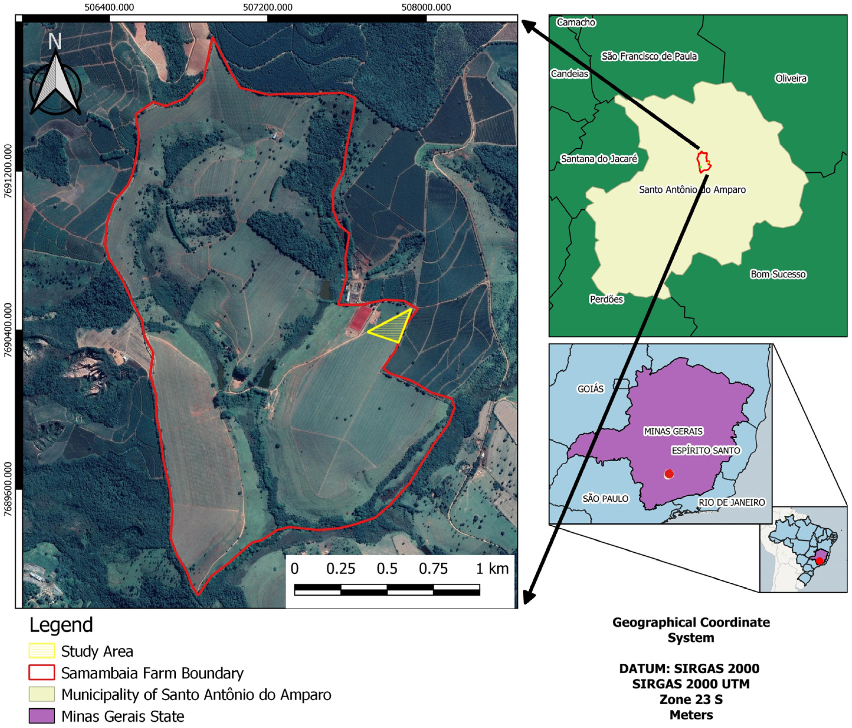
2.1. Study Area

The experiment was conducted at Samambaia Farm, located in the municipality of Santo Antônio do Amparo in the region of Campos das Vertentes, southeastern Minas Gerais [31]. The regional climate, according to the Köppen climate classification modified in [32], is Cwb, subtropical humid, with dry winters and temperate summers, mean temperatures ranging from 18 °C to 22 °C, and a mean annual rainfall of 1650 mm. The dry season stretches from May to September, and the rainy season normally lasts until late March or early April.
The study area (Figure 1) has 0.31 ha and an average altitude of 1026 m (a.s.l.), and it is located at the geographic coordinates 507,868.215 W and 7,690,442 S (longitude and latitude in meters) in the UTM zone, 23S projection and SIRGAS 2000 geodetic reference. Coffee seedlings of the cultivar Catucaí 2SL, species Coffea arabica L., were transplanted to this area. The soil of the region is red-yellow latosol [33].

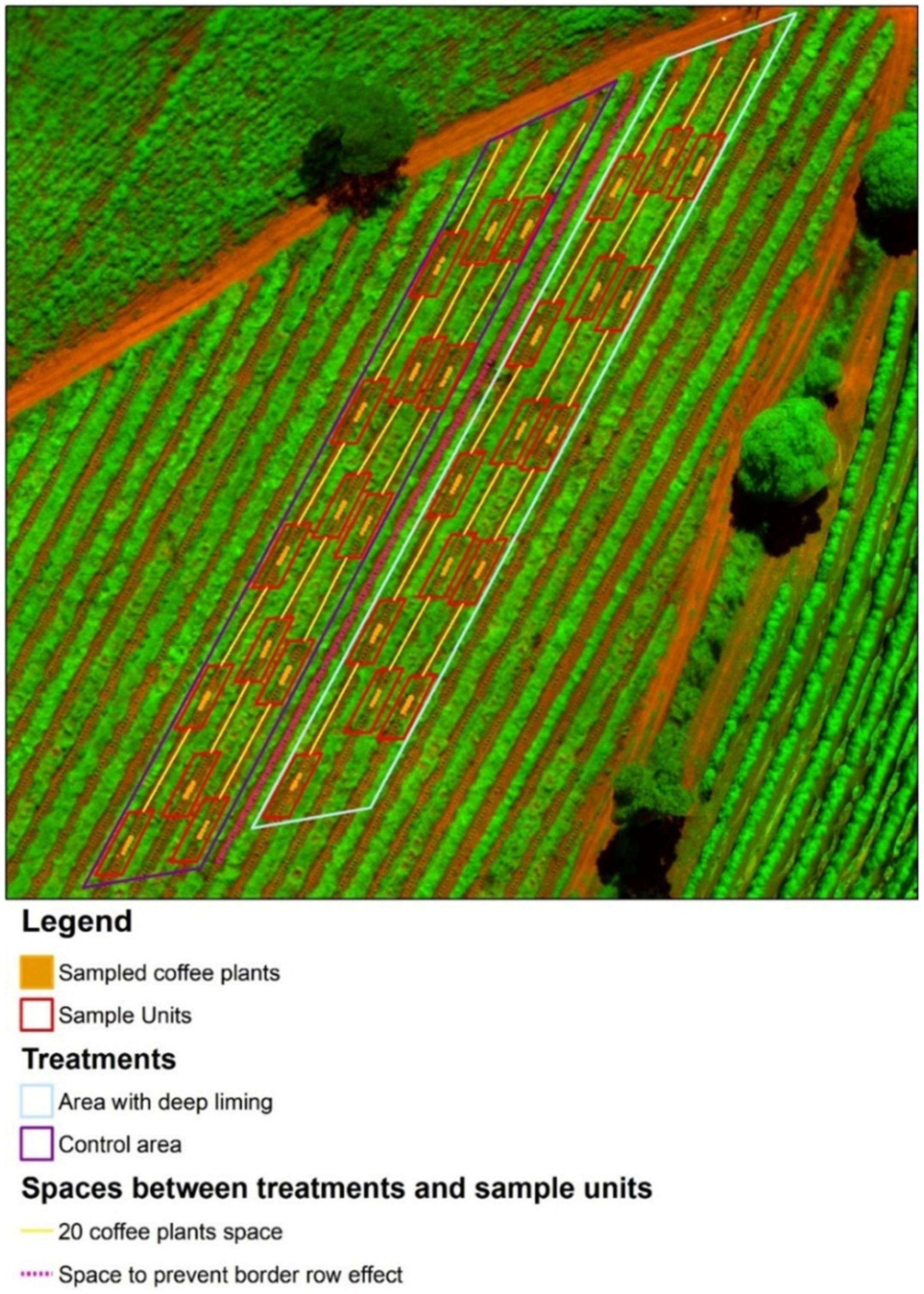
2.2. Crop Treatments and Transplanting

For coffee pre-planting, initially, a dose of 4 tons of dolomitic limestone per hectare was applied to the soil surface throughout the study area. This limestone was incorporated via disc harrowing, first with a heavy-duty disc harrow and then a lighter secondary disc harrow. Then, subsoiling was performed using a subsoiler type (Ikeda company, Marília, Brazil) with a 60 cm deep rod.
Subsequently, 35 cm deep furrows were opened, with 3.8 m spacing between rows, which were treated with gypsum, limestone, and magnesite doses (150 g/m, 600 g/m, and 100 g/m, respectively). Furrowing was repeated to incorporate the aforementioned inputs and to apply phosphate fertilizer (monoammonium phosphate (MAP)—200 g/m) and chicken manure (2000 g/m). Then, the furrows were closed using a 3-shank ripper, which also broke up the remaining clods. Last, 400 g/m dolomitic limestone was applied to the soil at depths ranging from 0.60 to 0.80 m using the implement inter-row weeder, leaving 3 rows without management, adopted as controls, to monitor this experiment.
Seedlings, previously grown in a nursery with 0.50 m × 3.8 m spacing (between plants and between rows, respectively), in perforated bags, were transplanted in November and December 2018 using a Mafes transplanter (Gralha model). Ground control points (GCPs) were used to mark the sample units to more easily identify them in the UAV images.

2.3. UAV, Flight Plans, and Multispectral Sensor

Aerial images were acquired with a UAV DJI Matrice 100, a quadcopter drone with rotating propellers, Wi-Fi connection to the base station, autonomous operation from 22 to 28 min, a 5 km range, and a 17 m/s maximum speed in Global Positioning System (GPS) mode [34].
The Precision Flight software (Version 1.3.2, Precision Hawk, Raleigh, NC, USA) [35] was used to plan the flight missions, in which the flight directions (across the rows), image overlay (80 × 80%), velocity (8 m/s), and height (50 m) were configured.
The images were acquired using the Parrot Sequoia sensor, which has an RGB sensor with a resolution of 16 megapixels (4608 × 3456) and four extra sensors with a resolution of 1.5 megapixels (1280 × 960) in the spectral bands of green (550 nm, BP 40), red (660 nm, BP 40), red-edge (735 nm, BP 10), and near-infrared (790 nm, BP 40). The camera was equipped with a solar radiation sensor coupled to a global navigation satellite system (GNSS) and a radiometric calibration panel to calibrate EMR and to standardize the data in reflectance values. The spatial resolution of the mosaics and the reflectance maps was 4.85 cm pixels.

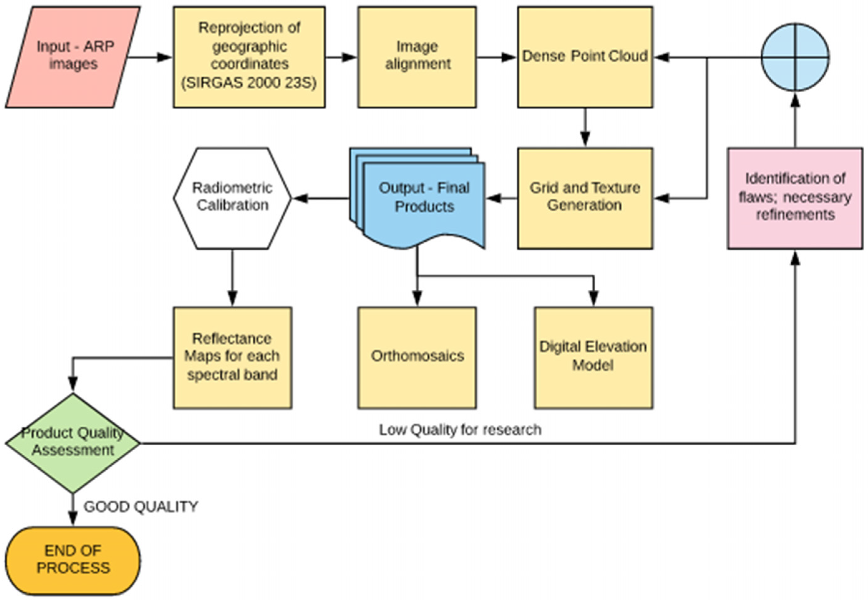
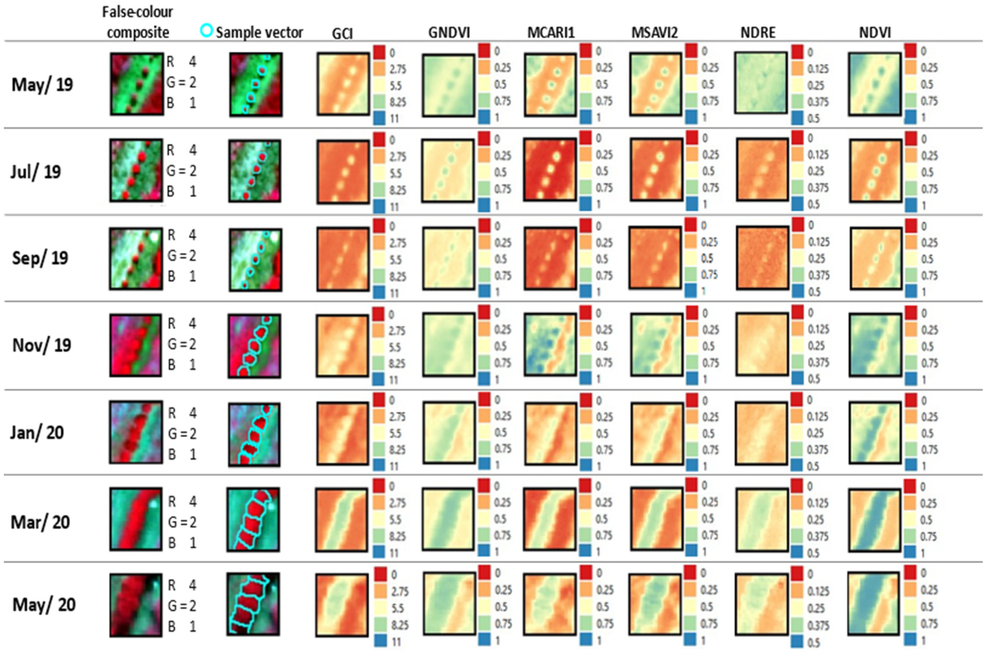
2.4. Image Processing and Spectral Data

The images were processed in the PIX4D Mapper software, version 4.4.10 [36], according to the process flow diagram shown in Figure 2. The QGIS 3.4.14 Madeira software [37] and eCognition Developer 9.0 [38] were used to generate Vis and segment images and produce and store geospatial vector data (shapefiles) on the coffee plant samples. The values of the parameters measured in the field—the height, crown diameter, and chlorophyll—were entered into the tables outlining the attributes of the vector data.
The parameters adopted in each image processing step are outlined in Table 1.

2.5. Vegetation Indices
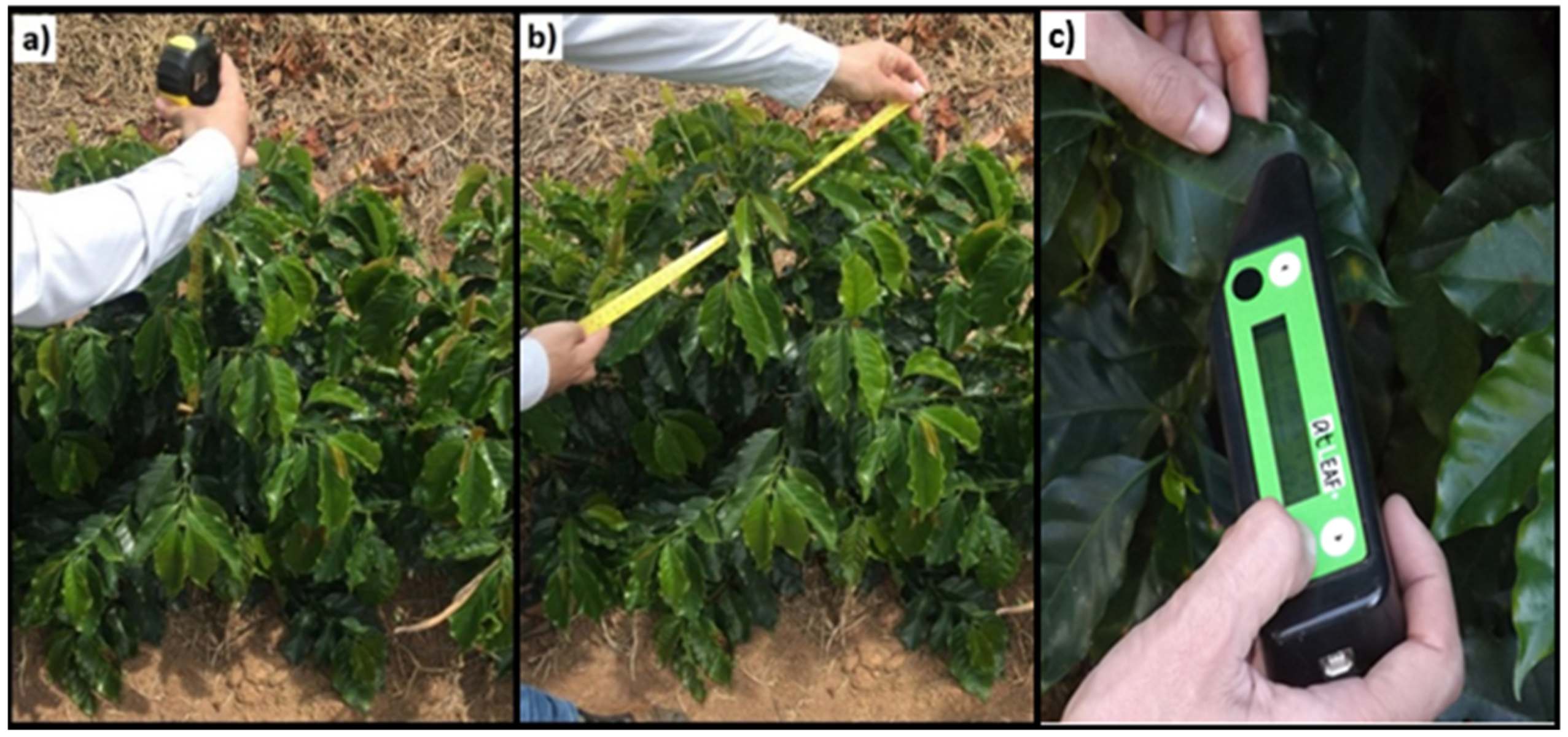
The following VIs were calculated to study the spectral responses of coffee plants subjected to different treatments: normalized difference vegetation index (NDVI), green NDVI (GNDVI), normalized difference red edge (NDRE), modified soil-adjusted vegetation index 2 (MSAVI2), modified chlorophyll absorption in reflectance index 1 (MCARI1), and green chlorophyll index (GCI) (Equations (1)–(6), respectively). These selected spectral indicators are commonly used to assess productivity based on the chlorophyll content, water stress, nitrogen, and vigor, among other factors [39,40,41,42,43].
NDVI = ρ nir ρ red ρ nir + ρ red
GNDVI = ρ nir ρ green ρ nir + ρ green
NDRE = ρ nir ρ red - edge ρ nir + ρ red - edge
MSAVI 2 = 0.5 × ( 2 ρ nir + 1 ) ( 2 ρ nir + 1 ) × 2 - 8 × ( ρ nir ρ red )
MCARI 1 = 1.5 × 2.5 ( 2 ρ nir ρ red ) - 1.3 ( 2 ρ nir ρ red )
CIg = ρ nir ρ green -   1
where: ρgreen—the reflectance in the green spectral range; ρred—the reflectance in the red spectral range; ρ(red-edge)—the reflectance in the red-edge spectral range; ρnir—the reflectance in the near-infrared spectral range.
The indices were calculated in QGIS using the “Raster Calculator” tool and extracted using the “Zonal Statistics” tool. The vectors were generated in the eCognition Developer software (version 9.0.1) using a process tree, according to [44], with the following sequence of tasks: image segmentation including “multi-resolution segmentation” and “spectral difference segmentation”; coffee plant sampling including “sample selection”; training and classification including “support vector machine” (parameters: brightness, shape, compactness, spectral bands, and VIs); and export of vectors in shapefile format.

2.6. Field Sampling

The plant height and crown diameter (average values in cm) measurements were taken with a graduated measuring tape, and the chlorophyll content was measured with a chlorophyll sensor (Figure 3) every two months on the same day of the flights.
The chlorophyll content was assessed using an atLEAF+ Chl meter (FT Green LLC, Wilmington, DE, USA), which returns dimensionless values. These values were converted into chlorophyll a and b contents using Equations (7) and (8), respectively [45].
Chl a = - 5.774   +   0.430   × atLEAF   +   0.0045   ×   atLEAF 2
Chl b = 0 . 040   ×   atLEAF 1.57
where atLEAF is the chlorophyll content recorded using the chlorophyll meter (dimensionless), C h l a is chlorophyll content a (μg/cm2), and C h l b is chlorophyll content b (μg/cm2).
The LAI was calculated according to the method in [46], using the plant height and crown diameter to relate the leaf area to the crop area (surface area occupied by the crop) according to Equation (9).
LAI = 0.0134 + 0.7276 × D 2 × h
where D is the plant diameter (m) and h is the plant height (m).
Samples were collected as shown in Figure 4. To evaluate the response of the coffee plants in an area with deep liming, in the treatment area, 3 rows were marked by dividing each row into 5 sampling units, each of which consisted of 5 sampled plants, on average, spaced apart by 20 plants, totaling 15 samples. In the control area, that is, with surface liming, the same procedure was followed with one row of spacing from the previously sampled area to prevent border row effects.

2.7. Meteorological Variables

Monthly cumulative rainfall and monthly mean temperature data were retrieved from the National Aeronautics and Space Administration (NASA) initiative, Prediction Of Worldwide Energy Resources (POWER) [47], to assess the effects of meteorological conditions on coffee growth.

2.8. Statistical Analysis

Data collected in the field and extracted from images were tabulated in the Microsoft Excel software (2013) [48], where graphs were also plotted to evaluate variations in coffee plants over time.
The Shapiro–Wilk test [49] was performed in the SISVAR software to assess data normality, resulting in non-parametric values. The data were submitted to the Mann–Whitney test [50], which is recommended for non-parametric variables, in the software environment R, with a significance level ρ = 0.05.
Spearman’s rank order correlation [51] ( ρ ^ s ) was calculated to evaluate the correlation levels between the parameters measured in the field and those extracted from the UAV images. Based on the most relevant correlations, a linear regression analysis was performed to predict the physical variables sampled in the field based on digital measurements from the UAV images. The models were developed in the software environment R [52].

3. Results and Discussion

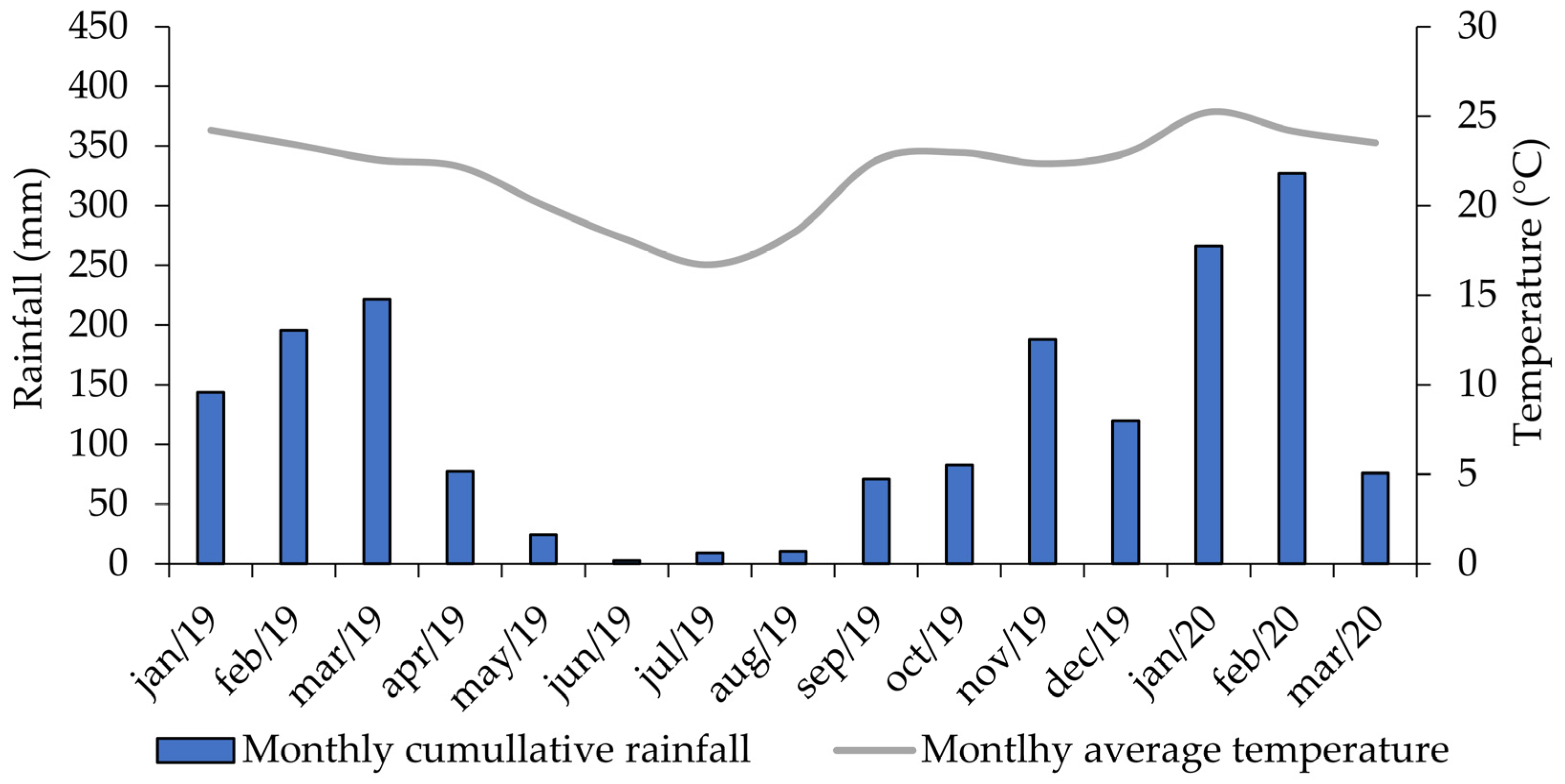
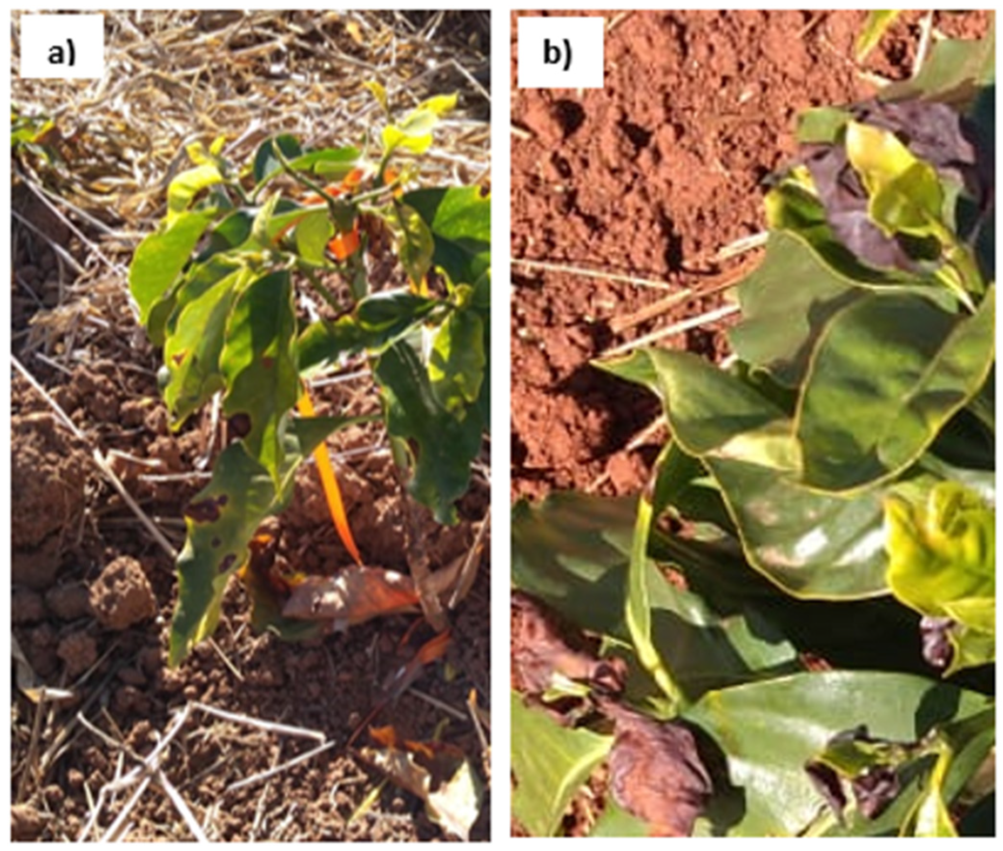
3.1. Temporal Analysis of Meteorological Conditions and Coffee Growth Response

A temporal analysis of the meteorological conditions during the coffee cycle can be seen in Figure 5. It is possible to observe variations in the cumulative rainfall and mean air temperature during the experiment. The highest accumulation of rain was observed in the summer, and the air temperature remained constant. On the other hand, in the winter, the volume of rain and the air temperature were reduced. Climatic conditions are of great importance in the period of establishment of seedlings in the field. According to the results presented, it is possible to highlight that the meteorological conditions were favorable for the establishment and growth of the coffee plants.
For a clearer understanding of the coffee plants’ temporal dynamics, images of the same plot of coffee plants during the study months can be seen in Figure 6, showing the VIs evaluated in this study and the false-color composite RGB 4, 2, and 1 (near infrared, red, and green, respectively), which were widely used to evaluate the leaf response in terms of vegetation.
The coffee growth variables and vegetation indices’ responses for the areas with deep liming and the areas with surface liming can be seen in Table 2. The results show the temporal variation in the studied variables, including the parameters measured via remote sensing, such as the VIs and canopy area calculated via vectorization, and the growth variables, such as the LAI and chlorophyll content, based on field sampling.
According to the results, after establishing the seedlings in the field, it was possible to observe linear increases in the values of the growth variables of height, crown diameter, LAI, and canopy area for the treatments with limestone on the surface and in depth. It was not possible to observe differences in the growth response between the studied treatments. This response may be associated with the effect of limestone on the soil, since the interaction and effect occur gradually and slowly, resulting in a more evident response throughout the crop cycle.
Figure 7 shows the damage on the plants caused by unfavorable conditions during dry and cool months. Since the photographs were recorded in July, the plants’ conditions can be associated with precipitation/temperature (Figure 5) and the spectral response (Table 2) over the sampled months, considering that plants normally take 30 to 60 days to respond to rainfall effects [53]. Therefore, in this study, with bimonthly measurements, the coffee crop year was divided into the dry season, from May to September, and the rainy season, from November to March.
In general, the physical measurements increased bimonthly, as shown by the variation in the LAI (derived from height and diameter), the canopy area calculated via vectorization, chlorophyll contents, and VIs. In September, the values of the LAI and canopy area calculated via vectorization stagnated, possibly due to winter defoliation. The LAI findings corroborate those of [46], which assessed a mean of 0.27 for the coffee plants after 15 months of planting, and [54], which showed a variation in the LAI over time similar to that found in the present study when studying evapotranspiration in young coffee plants.
The graphs also show that, in July and January, which are critical winter and summer months, the chlorophyll values were the highest and lowest, respectively. This response is related to the fact that under water stress, chloroplasts act to increase CO2 uptake to maintain the physiological activities of plants, thereby increasing the concentration of photosynthetic pigments whilst decreasing the leaf water content, which results in higher values in chlorophyll meter readings.
The VIs decreased during the dry season (from May to September) and increased again during the rainy season. The dry season is also when coffee plants grow the least because most of this period overlaps with winter, which is a period of stress during which photoassimilates were used to grow and maintain the root system to the detriment of vegetative growth, which also explains the drop in the VI values. In addition, the drop in temperature may damage the leaves, as shown in Figure 7, which is ultimately reflected in the values of the VIs. These occurrences corroborate the studies of [55,56,57], which also reported lower VI values in the satellite images of coffee plants during the dry season, especially in the winter, and in the monitoring of coffee trees that were recently transplanted via UAVs, as evidenced in [30].
During the rainy season, the values of the VIs increased again. Some of them, such as MCARI1 and MSAVI2, were higher in November than in January. This finding suggests that these indices were more sensitive to flowering in this experimental area. Flowering usually occurs between September and November, and despite its minimum intensity in new plants, such as the coffee seedlings sampled in this study (1 year after transplanting), it can affect the responses of the coffee plants, as shown in [58], which observed an increase in the VI values in colza crops, and in [59], which reported that the NDVI and enhanced vegetation index (EVI) of Coffea arabica peaked during flowering.
In general, the variation in the values of the VIs evaluated in this study is similar to the dynamics found in [59]. The author used the moderate resolution imaging spectroradiometer (MODIS) NDVI to propose an agrometeorological–spectral monitoring model based on the responses of coffee seedlings and mature and pruned coffee plants over time. Other studies reported a similar temporal variation when evaluating the VIs of coffee plants [55,56,60]. Therefore, although this experiment involves young coffee plants, this pattern can be associated with the phenological phases of the coffee tree reported in [61]. Nevertheless, the values of this VI are lower in young coffee plants than in adult coffee plants, primarily due to the lower biomass concentration [59,62].
In the evaluation of the difference between coffee plants subjected to different treatments, that is, deep and surface liming, in Table 2, no clear differences in variations over time are identified in most variables. The lack of differences related to growth and the LAI may be explained by the failure of the seedlings’ roots to reach depths of 70 to 80 cm (liming horizon) during the study period and thus benefit from the input. Only the chlorophyll parameter showed higher values in May and January, especially in the former, in the plantation treated with deep liming than in the plantation treated without deep liming.
The VIs of GCI, NDVI, and GNDVI, which are frequently associated with plant vigor and chlorophyll a, are slightly higher in the plantation with deep liming in the dry season. The ability to maintain plant vigor in periods of stress indicates limestone action. Liming decreases soil acidity, which increases nutrient availability, thereby providing nutrition to coffee plants during critical periods. Furthermore, the inter-row weeder, an implement used during liming, may have increased the soil porosity, favoring water infiltration and storage [9,63] whilst ensuring longevity and reducing losses.

3.2. Statistical Analysis for Coffee Growth Variables

To assess the differences between the transplanted coffee seedling growth of the treatments evaluated in this study, that is, deep liming vs. surface liming, the Mann–Whitney U test was performed at a significance level of p = 0.05.
Table 3 shows no significant differences between the treatments evaluated in this study, except for the chlorophyll parameter. The plantation with deep liming shows a higher chlorophyll concentration than that without deep liming. Therefore, although the other variables do not show any clear differences between managements, the chlorophyll meter can be an effective tool in identifying these differences in this type of evaluation. The U value (Mann–Whitney sum of ranks) of the plantation treated with deep liming is 8893.50 in contrast to 7396.50 in the plantation without deep liming, with a mean total chlorophyll (a + b) content of 86.04 μg/cm2 versus 83.87 μg/cm, respectively.
Few studies on deep liming in coffee plantations were found in the literature, especially long-term studies or research relating deep liming to VIs, thus requiring comparisons to other cultures. According to the authors of [15], who evaluated deep liming in olive trees, which is a perennial crop, as well as in coffee trees, the use of European soil, which has naturally lower pH values, is a requirement for the success of these plants. The authors observed an improvement in the soil’s physical–chemical attributes, but the only parameter with a positive and limiting correlation with productivity was the concentration of boron; that is, applying lime did not result in any significant differences compared to conventional planting. The authors [64] observed a 66% increase in root growth up to the 60 cm horizon by increasing the limestone dose in this profile and observed a 140% increase in production.
The authors of [65] evaluated different subsurface limestone doses for the Catuaí and Icatu varieties (up to 34 cm below the surface) in soils with a high aluminum content and observed increases in the total root length/root dry matter values (cm/g) and in the total root surface/root dry matter (cm2/g), in addition to a decrease in the aluminum content at the treatment site, mainly in the Catuaí cultivar. However, biophysical parameters such as the leaf area, stem length, and shoot dry matter production remained unaffected by management.
In [66], the authors evaluated coffee plants for one year after transplanting them to a cambisol subjected to furrowing or subsoiling and to different deep liming doses at 40, 60, and 80 cm and compared the results to those of coffee seedlings transplanted to soil without these preparations. All of the treatments resulted in physical and water improvements up to the 20 cm layer. The authors observed a better distribution of water and pore volume up to 40 cm in depth. The 80 cm deep liming stood out for its good water availability in this horizon, thus proving to be an alternative for mitigating possible damage caused by water deficits during the winter. The height and NDVI measurements were performed using a Green Seeker sensor, and the readings correlated well with the physical parameters measured in the field.
The study conducted in [66] showed that adopting treatments was effective, although no significant differences were found between the treatments regarding residual amounts of calcium and magnesium. These findings may therefore be associated with the soil factor because this natural cambisol had a high clay content, mainly below 20 cm of depth, in contrast to the latosol of the present study. Thus, the management adopted in comparison to the control represented a significant increase in the soil physical attributes rather than a chemical improvement related to liming.

3.3. Spearman’s Rank Correlation

To determine the degree of correlation between the physical variables measured in the field and those derived from the UAV images in this experiment, a Spearman’s rank correlation ( ρ ^ s ) analysis was performed, and the results are presented in Table 4.
All of the variables are positively correlated, except for chlorophyll, which has low or negative values across all correlated pairs. Some parameters stand out, such as the Vis of GCI, GNDVI, and NDVI. The latter has a 0.7627 correlation with the height of coffee plants growing in soil treated with deep liming, thus corroborating the findings of the authors of [66], who, when studying deep liming in coffee plantations, found that the Greenseeker NDVI was best correlated with height for liming at 60 cm of depth. The first two indices stand out, with correlation values close to 1 for parameters such as height, diameter, and LAI, which also have a correlation of 0.99 with the canopy area estimated in the software for both managements. The results indicate that these variables are good parameters for estimating or modeling some physical variables. Indices that use the green band have been applied in studies to estimate the biomass and other biophysical parameters in different crops [67,68]. The authors of [43] highlighted that the GNDVI, for example, is more sensitive to the chlorophyll concentration than the NDVI.
Other VIs do not obtain such promising correlation values, such as the MSAVI2, with moderate values (below 0.60), and the MCARI1 and NDRE, with low correlations ( ρ ^ s ) between 0.30 and 0.40, indicating that they are not good indices for monitoring coffee plants during development.
Following the non-parametric tests performed in the previous section, no major differences were found in the correlations between the study treatments, except for chlorophyll. Although low, the correlation between chlorophyll and extra-field parameters is more positive in the plantation with deep liming than in that without deep liming. The VI of NDRE has the highest value of correlation with this parameter ( ρ ^ s = 0.1705). The low correlations, even negative, with most of the VIs calculated in this study, may be related to the leaf sampling, which was performed randomly. According to [4], even in the same coffee tree, more exposed leaves (the outer section of plagiotropic branches or leaves located in the crown) are more susceptible to burning and chlorosis during periods of lower temperatures or may suffer more during intense summers. Conversely, the more internal leaves are more protected from these factors or may receive less solar radiation, and these factors affect the response of photosynthetic pigments.
The correlation values between the VIs and chlorophyll range from 0.55 to 0.78 in wheat [69]. For coffee plants, the authors of [20] developed models for predicting chlorophyll using Sentinel-2 images. The model developed by these authors explained 77% of the chlorophyll variation by using the 10 m bands of the sensor, unlike this study. The authors reported that mature coffee plants, older than 4 years, improved the model considerably compared to younger coffee plants because the near-infrared band of adult coffee plants is more reflective, and thus, the canopy area is more representative in the images. Young coffee plants, such as those sampled in this study, reduced the performance of the entire data set when modeling the total chlorophyll. Furthermore, the authors used, in addition to an SPAD chlorophyll meter, leaf samples of chlorophyll from the laboratory, which increased the accuracy of the readings.
Considering the VIs, UAV geometric measurements, and field measurements, both treatments performed similarly in this experiment. This result may be associated with the shallow root system of growing coffee plants, which therefore cannot benefit from deep liming. In turn, the positive correlation between most of the variables measured using UAVs—such as the VIs and geometric measurements—and the field measurements highlights the potential of using UAVs to estimate biophysical parameters, which shows the potential of this technology for monitoring coffee trees.
The authors suggest that further studies be carried out under conditions in which monitoring is carried out during the coffee plant’s adult stage, since the effect of deep liming treatment could be visible after a few seasons, which would require further monitoring. Also, deep liming could have a greater impact on coffee productivity instead of directly affecting the growth variables.

4. Conclusions

The results presented in this study contribute to Brazilian and world coffee growing. The use of remote sensing is widely used in agriculture. However, for coffee production areas, some gaps exist regarding the effectiveness of remote sensing in the evaluation of agricultural practices and the plant response after their establishment in the field. With our results, it is possible to observe that the use of VIs generated via multispectral images acquired using UAVs enabled the precise monitoring of the coffee crops after the seedlings were transplanted in the field. Also, the relationship between the evaluations performed in the field and the Vis’ results was satisfactory. Even when not observing the differences between the treatments studied—that is, liming application on the soil surface and in depth—this study showed a great applicability of remote sensing in the evaluation and monitoring of coffee crops.
Most of the variables determined using UAVs were highly correlated with the parameters measured in the field, except for chlorophyll, whose correlations were generally low or negative. The vegetation indices, particularly GCI, GNDVI, and NDVI, showed correlation values above 0.70 with the LAI and with the canopy area calculated via vectorization, whose correlation values with the LAI, crown diameter, and height were close to 1 in both treatments.

Author Contributions

Conceptualization, R.A.P.B. and G.A.e.S.F.; methodology and formal analysis, N.L.B., L.S.S., D.V.S. and D.G.M.; data curation, R.A.P.B., D.B.M. and L.S.S.; writing—original draft preparation, R.A.P.B.; writing—review and editing, L.C., G.B., G.R. and F.S.; visualization, D.B.M., D.G.M. and N.L.B.; supervision, G.A.e.S.F., L.C., G.B., G.R. and F.S.; project administration, R.A.P.B. All authors have read and agreed to the published version of the manuscript.

Funding

This study was funded by Embrapa Café-Consórcio Pesquisa Café (project 10.18.20.041.00.00), the National Council for Scientific and Technological Development (CNPq) (project 305953/2020-6) and the Minas Gerais Research Support Foundation (FAPEMIG) (projects PPE-00118-22 and BPD-00040-22).

Data Availability Statement

The data presented in this study are available upon request from the corresponding authors. The data are not publicly available.

Acknowledgments

We would like to thank the Federal University of Lavras (UFLA) and the Postgraduate Program in Agricultural Engineering (PPGEA), Embrapa Café-Consórcio Pesquisa Café, the National Council for Scientific and Technological Development (CNPq), the Minas Gerais Research Support Foundation (FAPEMIG), the Coordination of Improvement of Higher Education Personnel (CAPES), and University of Firenze for support this research development.

Conflicts of Interest

The authors declare no conflict of interest.

References

  1. Latini, A.O.; Silva, D.P.; Souza, F.M.L.; Ferreira, M.C.; Moura, M.S.; Suarez, N.F. Reconciling coffee productivity and natural vegetation conservation in an agroecosystem landscape in Brazil. J. Nat. Conserv. 2020, 57, 125902. [Google Scholar] [CrossRef]
  2. Méndez Rodríguez, C.; Salazar Benítez, J.; Rengifo Rodas, C.F.; Corrales, J.C.; Figueroa Casas, A. A multidisciplinary approach integrating emergy analysis and process modeling for agricultural systems sustainable management—Coffee farm validation. Sustainability 2022, 14, 8931. [Google Scholar] [CrossRef]
  3. Ferraz, G.A.S.; Silva, F.M.; Costa, P.A.N.; Silva, A.C.; Carvalho, F.D.M. Precision agriculture to study soil chemical properties and the yield of a coffee field. Coffee Sci. 2012, 7, 59–67. [Google Scholar]
  4. Mesquita, C.M.D.; Rezende, J.D.; Carvalho, J.S.; Fabri Júnior, M.A.; Moraes, N.C.; Dias, P.T.; Araújo, W.D. Manual do Café: Manejo de Cafezais em Produção; Emater-MG: Belo Horizonte, Brazil, 2016; pp. 1–52. [Google Scholar]
  5. Nora, D.D.; Amado, T.J.C. Improvement in chemical attributes of Oxisol subsoil and crop yields under no-till. Agron. J. 2013, 105, 1393–1403. [Google Scholar] [CrossRef]
  6. Raij, B. Gesso na Agricultura. Campinas; Instituto Agronômico: Belo Horizonte, Brazil, 2008; 233p. [Google Scholar]
  7. Rheinheimer, D.D.; Santos, E.J.S.; Kaminski, J.; Bortoluzzi, E.C.; Gatiboni, L.C. Alterações de atributos do solo pela calagem superficial e incorporada a partir de pastagem natural. Rev. Bras. Cienc. Solo 2000, 24, 797–805. [Google Scholar] [CrossRef]
  8. Amaral, A.S.; Anghinoni, I. Alteração de parâmetros químicos do solo pela reaplicação superficial de calcário no sistema plantio direto. Pesqui. Agropecu. Bras. 2001, 36, 695–702. [Google Scholar] [CrossRef]
  9. Serafim, M.E.; Lima, J.M.D.; Lima, V.M.P.; Zeviani, W.M.; Pessoni, P.T. Alterações físico-químicas e movimentação de íons em Latossolo gibbsítico sob doses de gesso. Bragantia 2012, 71, 75–81. [Google Scholar] [CrossRef]
  10. Vitti, G.C.; Luz, P.H.D.C.; Malavolta, E.; Dias, A.S.; Serrano, C.G.D.E. Uso do Gesso em Sistemas de Produção Agrícola; GAPE: Piracicaba, Brazil, 2008; 104p. [Google Scholar]
  11. Pereira, F.S. Gesso de Minério Associado a Fontes de Fósforo na Cultura do Milho em Sistema Plantio Direto no Estado de Alagoas; Universidade Estadual Paulista “Júlio de Mesquita Filho”: Botucatu, Brazil, 2007; 67p. [Google Scholar]
  12. Prado, R.M.; Natale, W. Uso da grade aradora superpesada, pesada e arado de discos na incorporação de calcário em profundidade e na produção de milho. Eng. Agríc. 2004, 24, 167–176. [Google Scholar] [CrossRef]
  13. Ferreira, D.F. Sisvar: A computer statistical analysis system. Ciênc. Agrotec. 2011, 35, 1039–1042. [Google Scholar] [CrossRef]
  14. Garcia, C.P. Efeitos do Preparo Profundo do Solo e da Calagem na Compactação do Solo e na Produtividade da Cana-de-Açúcar; Universidade Estadual Paulista “Julio de Mesquita Filho”: Botucatu, Brazil, 2018; 96p. [Google Scholar]
  15. Bender, D.D.B.B.; Weber, M.A.; Vieira, F.C.B. Necessidade de ajustes no sistema de recomendação de calagem e adubação de oliveiras (Olea europaea L.) no sul do Brasil. Rev. Ecol. Nutr. Florest. 2018, 6, 17–32. [Google Scholar] [CrossRef]
  16. Li, G.; Wan, S.; Zhou, J.; Yang, Z.; Qin, P. Leaf chlorophyll fluorescence, hyperspectral reflectance, pigments content, malondialdehyde and proline accumulation responses of castor bean (Ricinus communis L.) seedlings to salt stress levels. Ind. Crops Prod. 2010, 31, 13–19. [Google Scholar] [CrossRef]
  17. Mahajan, G.R.; Sahoo, R.N.; Pandey, R.N.; Gupta, V.K.; Kumar, D. Using hyperspectral remote sensing techniques to monitor nitrogen, phosphorus, sulphur and potassium in wheat (Triticum aestivum L.). Precis. Agric. 2014, 15, 499–522. [Google Scholar] [CrossRef]
  18. Nebiker, S.; Annen, A.; Scherrer, M.; Oesch, D. A light-weight multispectral sensor for micro UAV—Opportunities for very high resolution airborne remote sensing. ISPRS Arch. 2008, 37, 1193–1199. [Google Scholar]
  19. Chemura, A.; Mutanga, O.; Dube, T. Remote sensing leaf water stress in coffee (Coffea arabica) using secondary effects of water absorption and random forests. Phys. Chem. Earth 2017, 100, 317–324. [Google Scholar] [CrossRef]
  20. Chemura, A.; Mutanga, O.; Dube, T. Integrating age in the detection and mapping of incongruous patches in coffee (Coffea arabica) plantations using multi-temporal Landsat 8 NDVI anomalies. Int. J. Appl. Earth Obs. Geoinf. 2017, 57, 1–13. [Google Scholar] [CrossRef]
  21. Katsuhama, N.; Imai, M.; Naruse, N.; Takahashi, Y. Discrimination of areas infected with coffee leaf rust using a vegetation index. Remote Sens. Lett. 2018, 9, 1186–1194. [Google Scholar] [CrossRef]
  22. Marin, D.B.; Carvalho Alves, M.; Pozza, E.A.; Belan, L.L.; Oliveira Freitas, M.L. Multispectral radiometric monitoring of bacterial blight of coffee. Precis. Agric. 2019, 20, 959–982. [Google Scholar] [CrossRef]
  23. Marin, D.B.; Alves, M.D.C.; Pozza, E.A.; Gandia, R.M.; Cortez, M.L.J.; Mattioli, M.C. Sensoriamento remoto multiespectral na identificação e mapeamento das variáveis bióticas e abióticas do cafeeiro. Rev. Ceres 2019, 66, 142–153. [Google Scholar] [CrossRef]
  24. Carrijo, G.L.; Oliveira, D.E.; Assis, G.A.; Carneiro, M.G.; Guizilini, V.C.; Souza, J.R. Automatic detection of fruits in coffee crops from aerial images. In Proceedings of the Latin American Robotics Symposium (LARS) and 2017 Brazilian Symposium on Robotics (SBR), Curitiba, Brazil, 8–11 November 2017; pp. 1–6. [Google Scholar]
  25. Oliveira, H.C.; Guizilini, V.C.; Nunes, I.P.; Souza, J.R. Failure Detection in Row Crops from UAV Images Using Morphological Operators. IEEE Geosci. Remote Sens. Lett. 2018, 7, 991–995. [Google Scholar] [CrossRef]
  26. Santos, L.M.; Souza Barbosa, B.D.; Diotto, A.V.; Andrade, M.T.; Conti, L.; Rossi, G. Determining the leaf area index and percentage of area covered by coffee crops using UAV RGB images. IEEE J. Sel. Top. Appl. Earth Obs. Remote Sens. 2020, 13, 6401–6409. [Google Scholar] [CrossRef]
  27. Marin, D.B.; Ferraz, G.A.E.S.; Guimaraes, P.H.S.; Schwerz, F.; Santana, L.S.; Barbosa, B.D.S.; Rossi, G. Remotely Piloted Aircraft and Random Forest in the evaluation of the spatial variability of foliar nitrogen in coffee crop. Remote Sens. 2021, 13, 1471. [Google Scholar] [CrossRef]
  28. Marin, D.B.; Ferraz, G.A.E.S.; Schwerz, F.; Barata, R.A.P.; Oliveira, F.R.; Dias, J.E.L. Unmanned aerial vehicle to evaluate frost damage in coffee plants. Precis. Agric. 2021, 22, 1845–1860. [Google Scholar] [CrossRef]
  29. Santana, L.S.; Ferraz, G.A.E.S.; Cunha, J.P.B.; Santana, M.S.; Faria, R.D.O.; Marin, D.B.; Sarri, D. Monitoring Errors of Semi-Mechanized Coffee Planting by Remotely Piloted Aircraft. Agronomy 2021, 11, 1224. [Google Scholar] [CrossRef]
  30. Bento, N.L.; Ferraz, G.A.E.S.; Barata, R.A.P.; Soares, D.V.; Santos, L.M.D.; Santana, L.S.; Palchetti, E. Characterization of Recently Planted Coffee Cultivars from Vegetation Indices Obtained by a Remotely Piloted Aircraft System. Sustainability 2022, 14, 1446. [Google Scholar] [CrossRef]
  31. Baruqui, A.M.A.; Naime, U.J.; Motta, P.E.F.; Carvalho Filho, A.D. Levantamento de Reconhecimento de Média Intensidade dos Solos da Zona Campos das Vertentes-MG; Boletim de Pesquisa e Desenvolvimento; Embrapa Solos: Rio de Janeiro, Brazil, 2006; 134p. [Google Scholar]
  32. Alvares, C.A.; Stape, J.L.; Sentelhas, P.C.; Gonçalves, J.D.M.; Sparovek, G. Köppen’s climate classification map for Brazil. Meteorol. Zeitschrift. 2013, 22, 711–728. [Google Scholar] [CrossRef]
  33. EMBRAPA—Empresa Brasileira de Pesquisa Agropecuária. Sistema Brasileiro de Classificação de Solos; Embrapa-SPI: Rio de Janeiro, Brazil, 2006; 412p. [Google Scholar]
  34. DJI. DJI MATRICE 100—User Manual. 2016. Available online: https://dl.djicdn.com/downloads/m100/M100_User_Manual_EN.pdf (accessed on 10 May 2022).
  35. Precisionhawk. Precision Flight Free—Turn Your Drone into an Advanced Remote Sensing Tool—Features. 2017. Available online: https://www.precisionhawk.com/precisionflight (accessed on 11 March 2022).
  36. PIX4D SA. Pix4D Mapper 4.4.10. 2019. Available online: https://www.pix4d.com/product/pix4dmapper-photogrammetry-software (accessed on 25 March 2022).
  37. Qgis Development Team. QGIS Geographic Information System; Open Source Geospatial Foundation Project: Beaverton, OR, USA, 2019. [Google Scholar]
  38. Trimble. Ecognition Developer 9.0 User Guide; Trimble Germany GmbH: Munich, Germany, 2014. [Google Scholar]
  39. DaMatta, F.M.; Godoy, A.G.; Menezes-Silva, P.E.; Martins, S.C.; Sanglard, L.M.; Morais, L.E.; Ghini, R. Sustained enhancement of photosynthesis in coffee trees grown under free-air CO2 enrichment conditions: Disentangling the contributions of stomatal, mesophyll, and biochemical limitations. J. Exp. Bot. 2016, 67, 341–352. [Google Scholar] [CrossRef]
  40. Haboudane, D.; Miller, J.R.; Pattey, E.; Zarco-Tejada, P.J.; Strachan, I.B. Hyperspectral vegetation indices and novel algorithms for predicting green LAI of crop canopies: Modeling and validation in the context of precision agriculture. Remote Sens. Environ. 2004, 90, 337–352. [Google Scholar] [CrossRef]
  41. Gitelson, A.A.; Gritz, Y.; Merzlyak, M.N. Relationships between leaf chlorophyll content and spectral reflectance and algorithms for non-destructive chlorophyll assessment in higher plant leaves. J. Plant Physiol. 2003, 160, 271–282. [Google Scholar] [CrossRef]
  42. Barnes, E.M.; Clarke, T.R.; Richards, S.E.; Colaizzi, P.D.; Haberland, J.; Kostrzewski, M.; Moran, M.S. Coincident detection of crop water stress, nitrogen status and canopy density using ground based multispectral data. In Proceedings of the 5th International Conference on Precision Agriculture, Bloomington, MN, USA, 16–19 July 2000. [Google Scholar]
  43. Gitelson, A.A.; Kaufman, Y.J.; Merzlyak, M.N. Use of a green channel in remote sensing of global vegetation from EOS-MODIS. Remote Sens. Environ. 1996, 58, 289–298. [Google Scholar] [CrossRef]
  44. Benz, U.C.; Hofmann, P.; Willhauck, G.; Lingenfelder, I.; Heynen, M. Multi-resolution, object-oriented fuzzy analysis of remote sensing data for GIS-ready information. ISPRS J. Photogramm. Remote Sens. 2004, 58, 239–258. [Google Scholar] [CrossRef]
  45. Padilla, F.M.; Souza, R.; Peña-Fleitas, M.T.; Gallardo, M.; Giménez, C.; Thompson, R.B. Different responses of various chlorophyll meters to increasing nitrogen supply in sweet pepper. Front. Plant Sci. 2018, 9, 1752. [Google Scholar] [CrossRef] [PubMed]
  46. Favarin, J.L.; Dourado Neto, D.; García, A.G.; Nova, N.A.V.; Favarin, D.G. Equations for estimating the coffee leaf area index. Pesqui. Agropecu. Bras. 2002, 37, 769–773. [Google Scholar] [CrossRef]
  47. National Aeronautics and Space Administration—NASA. Power Data Access Viewer. 2020. Available online: https://power.larc.nasa.gov/data-access-viewer/ (accessed on 20 August 2020).
  48. Microsoft. Microsoft Excel—Computer Software; Microsoft Corporation: Washington, DC, USA, 2013. [Google Scholar]
  49. Shapiro, S.S.; Wilk, M.B. An analysis of variance test for normality (complete samples). Biometrika 1965, 52, 591–611. [Google Scholar] [CrossRef]
  50. Mann, H.B.; Whitney, D.R. On a test of whether one of two random variables is stochastically larger than the other. Ann. Math. Stat. 1947, 18, 50–60. [Google Scholar] [CrossRef]
  51. Spearman, C. The Proof and Measurement of Association between Two Things. Am. J. Psychol. 1904, 15, 72–101. [Google Scholar] [CrossRef]
  52. R Development Core Team. R: A Language and Environment for Statistical Computing; R Foundation for Statistical Computing: Vienna, Austria, 2009. [Google Scholar]
  53. Braga, C.C.; Brito, J.D.; Sansigolo, C.A.; Rao, T.V.R. Tempo de resposta da vegetação às variabilidades sazonais da precipitação no Nordeste do Brasil. Rev. Bras. Meteorol. 2003, 11, 149–157. [Google Scholar]
  54. Flumignan, D.L.; De Faria, R.T. Evapotranspiração e coeficientes de cultivo de cafeeiros em fase de formação. Bragantia 2009, 68, 269–278. [Google Scholar] [CrossRef]
  55. Coltri, P.P.; Romani, L.A.S.; Dubreuil, V.; Corgne, S.; Zullo, J.J.; Pinto, H.S. Variação temporal da biomassa do café arábica arborizado e a pleno sol, através de índices de vegetação. In Proceedings of the 15th Simpósio Brasileiro de Sensoriamento Remoto, Curitiba, Brazil, 30 April–5 May 2011; INPE: São José dos Campos, Brazil, 2011. [Google Scholar]
  56. Volpato, M.; Alves, H.; Vieira, T.; Souza, W.D.O. Imagens MODIS para determinação de estiagem agrícola em área cafeeira no município de Patrocínio, MG. In Proceedings of the 14th Simpósio Brasileiro de Sensoriamento Remoto, Natal, Brazil, 25–30 April 2009; INPE: São José dos Campos, Brazil, 2009. [Google Scholar]
  57. Bernardes, T.; Moreira, M.A.; Adami, M.; Giarolla, A.; Rudorff, B.F.T. Monitoring Biennial Bearing Effect on Coffee Yield Using MODIS Remote Sensing Imagery. Remote Sens. 2012, 4, 2492–2509. [Google Scholar] [CrossRef]
  58. Fang, S.; Tang, W.; Peng, Y.; Gong, Y.; Dai, C.; Chai, R.; Liu, K. Remote estimation of vegetation fraction and flower fraction in oilseed rape with unmanned aerial vehicle data. Remote Sens. 2016, 8, 416. [Google Scholar] [CrossRef]
  59. Rosa, V.G.C. Modelo Agrometeorológico-Espectral para Monitoramento e Estimativa da Produtividade do Café na Região Sul/Sudoeste do Estado de Minas Gerais; INPE: São José dos Campos, Brazil, 2007; 142p. [Google Scholar]
  60. Júnior, A.F.C.; Carvalho Júnior, O.A.; Souza Martins, E.; Guerra, A.F. Phenological characterization of coffee crop (Coffea arabica L.) from Modis time series. Braz. J. Geol. 2013, 31, 569–578. [Google Scholar] [CrossRef]
  61. Camargo, A.P.; Camargo, M.B.P. Definição e esquematização das fases fenológicas do cafeeiro arábica nas condições tropicais do Brasil. Bragantia 2001, 60, 65–68. [Google Scholar] [CrossRef]
  62. Wu, J.; Wang, D.; Bauer, M.E. Assessing broadband vegetation indices and QuickBird data in estimating leaf area index of corn and potato canopies. Field Crops Res. 2007, 102, 33–42. [Google Scholar] [CrossRef]
  63. Nolla, A.; Silva, V.L.B.; Muniz, A.S.; Silva, T.R.B. Correção da acidez do solo em profundidade através do uso de carbonatos, silicatos e casca de arroz em lisímetros. Rev. Cult. Sab. 2010, 3, 33–40. [Google Scholar]
  64. Caires, E.F.; Corrêa, J.C.L.; Churka, S.; Barth, G.; Garbuio, F.J. Surface application of lime ameliorates subsoil acidity and improves root growth and yield of wheat in an acid soil under no-till system. Sci. Agric. 2006, 63, 502–509. [Google Scholar] [CrossRef]
  65. Rodrigues, A.L.; Martinez, H.E.; Neves, J.C.L.; Novais, R.F.; Mendonça, S.M. Growth response of coffee tree shoots and roots to subsurface liming. Plant Soil 2001, 234, 207–214. [Google Scholar] [CrossRef]
  66. Barbosa, S.M.; Silva, B.M.; Oliveira, G.C.; Benevenute, P.A.N.; Silva, R.F.; Curi, N.; Pereira, V.M. Deep furrow and additional liming for coffee cultivation under first year in a naturally dense inceptisol. Geoderma 2020, 357, 113934. [Google Scholar] [CrossRef]
  67. Gutiérrez-Rodríguez, M.; Reynolds, M.P.; Escalante-Estrada, J.A.; Rodríguez-González, M.T. Association between canopy reflectance indices and yield and physiological traits in bread wheat under drought and well-irrigated conditions. Aust. J. Agric. Res. 2004, 55, 1139–1147. [Google Scholar] [CrossRef]
  68. Shanahan, J.F.; Schepers, J.S.; Francis, D.D.; Varvel, G.E.; Wilhelm, W.W.; Tringe, J.M.; Major, D.J. Use of remote-sensing imagery to estimate corn grain yield. Agron. J. 2001, 93, 583–589. [Google Scholar] [CrossRef]
  69. Hassan, M.A.; Yang, M.; Rasheed, A.; Jin, X.; Xia, X.; Xiao, Y.; He, Z. Time-series multispectral indices from unmanned aerial vehicle imagery reveal senescence rate in bread wheat. Remote Sens. 2018, 10, 809. [Google Scholar] [CrossRef]
Figure 1. Location map of the study area.
Agronomy 13 02623 g001
Figure 2. Flowchart of the UAV image processing in the software.
Agronomy 13 02623 g002
Figure 3. Field measurements of coffee plant height (a) and crown diameter (b); the chlorophyll meter used to measure the chlorophyll content in coffee leaves (c).
Agronomy 13 02623 g003
Figure 4. Schematic representation of the coffee plant sampling for the treatment and control areas.
Agronomy 13 02623 g004
Figure 5. Rainfall and air temperature variation during the experiment.
Agronomy 13 02623 g005
Figure 6. Visual representation of the bimonthly evolution of the VIs, including GCI, GNDVI, MCARI1, MSAVI2, NDRE, and NDVI in a plot, obtained using the false-color composite RGB = 4, 2, 1.
Agronomy 13 02623 g006
Figure 7. Photographs recorded in the field in July, which illustrate leaf damage caused by cold temperatures, resulting in defoliation, loss of vigor (a), and burning (b).
Agronomy 13 02623 g007
Table 1. Parameters used in the image processing flow of the Pix4D software (Mapper version 4.4.12).
ParameterConfiguration
Initial processing (alignment)
Keypoint image scaleFull
Matching image pairsAerial grid or corridor
Number of keypointsAutomatic
Calibration methodAlternative
Point cloud and mesh texture
Image scaleOriginal image size
Point densityHigh
Minimum number of matches3
3D textured meshHigh resolution
DSM and orthomosaic
ResolutionAutomatic
OrthomosaicGeoTIFF
Reflectance maps and index calculation
Radiometric calibrationIrradiance sensor and
calibration grid
BandsGreen, red, red edge, near infrared
ResolutionAutomatic
Reflectance mapGeoTIFF
Table 2. Coffee growth variables including height, crown diameter, chlorophyll content, LAI, chlorophyll a, chlorophyll b, total chlorophyll (a + b), and canopy area and the VIs, including the GCI, MSAVI2, MCARI1, GNDVI, NDRE, and NDVI, of the coffee seedlings transplanted to areas treated with deep liming and with surface liming.
Sampled Months
VariablesMayJulySeptemberNovemberJanuaryMarch
Treatment with deep liming
Height (cm)31.0135.7239.8750.3555.0770.45
Crown diameter (cm)29.4930.4531.6549.2458.6981.01
Chlorophyll content (IRC)69.9573.3659.8064.5559.8165.41
LAI0.03560.04080.04600.11220.16390.3715
Chlorophyll a (μg/cm2)46.759450.193536.448640.841836.139041.7047
chlorophyll b (μg/cm2)31.779134.079524.916727.844124.704328.4203
Total chlorophyll (μg/cm2)80.060086.039062.209569.747261.601071.2432
Canopy area (cm2)631.56777.16721.661583.751729.223725.61
GCI3.90452.92152.93824.33894.30036.7518
MSAVI20.55260.36040.29270.65160.49910.6086
MCARI10.56480.31930.24250.68300.45110.5375
GNDVI0.65410.58240.58730.67870.67390.7660
NDRE0.31580.14510.11430.19020.22300.3244
NDVI0.70320.51320.56470.78650.77990.8462
Treatment with surface liming
Height (cm)33.1635.5340.2550.1154.3369.11
Crown diameter (cm)31.8730.5732.9850.1758.4478.22
Chlorophyll content (IRC)60.2072.2059.2062.9756.9867.28
LAI0.04140.04140.05180.12150.16590.3500
Chlorophyll a (μg/cm2)36.689648.946235.877839.229633.392643.6815
chlorophyll b (μg/cm2)25.079133.249324.537026.766822.870329.7396
Total chlorophyll (μg/cm2)62.601683.867061.229266.943556.853274.6893
Canopy area (cm2)614.84824.29818.971647.601925.713825.22
GCI3.93892.76372.51804.31644.35296.6507
MSAVI20.54910.34960.25790.68110.51880.5990
MCARI10.55610.30950.20970.73710.47210.5320
GNDVI0.65510.56970.55100.67520.67490.7607
NDRE0.30950.13980.11400.19570.21780.3244
NDVI0.70470.50210.51060.80140.79160.8311
Table 3. Results of Mann–Whitney U test for non-parametric distributions assessing the existence of significant differences between plantations with and without deep liming.
Study VariableNull Hypothesis (H0)Mean RankU Value (Sum of Ranks)Significance Value pDecision
Height (cm)The distribution of the variable is the same for the different managementsSL = 91.33
DL = 89.67
8219.50
8070.50
0.831Accepts the null hypothesis (H0)
Diameter (cm) The distribution of the variable is the same for the different managementsSL = 92.88
DL = 88.12
8359.00
7931.00
0.540Accepts the null hypothesis (H0)
LAIThe distribution of the variable is the same for the different managementsSL = 93.98
DL = 87.02
8458.00
7832.00
0.371Accepts the null hypothesis (H0)
Chlorophyll a + b (μg/cm2)The distribution of the variable is the same for the different managementsSL = 82.18b
DL = 98.82a
7396.50b
8893.50a
0.032 *Rejects the null hypothesis (H0); the managements differ
Estimated crown area (cm2)The distribution of the variable is the same for the different managementsSL = 93.43
DL = 87.57
8409.00
7881.00
0.450Accepts the null hypothesis (H0)
GCIThe distribution of the variable is the same for the different managementsSL = 88.91
DL = 92.09
8002.00
8288.00
0.682Accepts the null hypothesis (H0)
MSAVI2The distribution of the variable is the same for the different managementsSL = 90.03
DL = 90.97
8103.00
8187.00
0.904Accepts the null hypothesis (H0)
MCARI1The distribution of the variable is the same for the different managementsSL = 90.11
DL = 90.89
8110.00
8180.00
0.920Accepts the null hypothesis (H0)
GNDVIThe distribution of the height variable is the same for the different managementsSL = 88.32
DL = 92.68
7949.00
8341.00
0.575Accepts the null hypothesis (H0)
NDREThe distribution of the variable is the same for the different managementsSL = 89.78
DL = 91.22
8080.00
8210.00
0.852Accepts the null hypothesis (H0)
NDVIThe distribution of the variable is the same for the different managementsSL = 88.58
DL = 92.42
7972.00
8318.00
0.621Accepts the null hypothesis (H0)
* Significant differences at the significance level ρ = 0.05; SL= surface liming; DL= deep liming.
Table 4. Spearman’s rank correlation ( ρ ^ s ) between the variables measured in the field and the variables assessed in UAV images of seedling plantations with deep liming and without deep liming.
Field Parameters
VIs (UAV)Height (cm)Crown Diameter (cm)Chlorophyll Content (IRC)LAIChlorophyll a (μg/cm2)Chlorophyll b (μg/cm2)Chlorophyll a + b (μg/cm2)
Treatment with deep liming
GCI0.87350.9281−0.13370.9525−0.1625−0.1624−0.1654
MSAVI0.51170.59110.04400.52900.01390.01370.0106
MCARI10.33200.40880.09750.33510.07070.07050.0678
GNDVI0.83930.9033−0.17800.8943−0.2076−0.2077−0.2107
NDRE0.38580.52630.18730.57560.17050.17020.1685
NDVI0.76270.8199−0.34150.7462−0.3701−0.3703−0.3732
Crown area0.95830.9753−0.20970.9953−0.2385−0.2384−0.2413
Treatment without deep liming
GCI0.86880.92240.08500.93240.06190.06180.0594
MSAVI0.51670.5953−0.06400.5128−0.0932−0.0936−0.0966
MCARI10.36300.4362−0.09030.3419−0.1187−0.1190−0.1220
GNDVI0.80760.8787−0.02380.8541−0.0492−0.0494−0.0521
NDRE0.44740.5621−0.04990.5927−0.0673−0.0671−0.0689
NDVI0.73140.7993−0.26050.7102−0.2877−0.2881−0.2909
Crown area0.97400.97760.17970.99740.16100.16070.1588
Disclaimer/Publisher’s Note: The statements, opinions and data contained in all publications are solely those of the individual author(s) and contributor(s) and not of MDPI and/or the editor(s). MDPI and/or the editor(s) disclaim responsibility for any injury to people or property resulting from any ideas, methods, instructions or products referred to in the content.

