Abstract
Thermogravimetric analysis (TGA) is becoming popular for the evaluation of biomass to determine the content of ashes, volatiles, and fixed carbon and to simulate pyrolysis, gasification, and combustion processes. This analysis consists of heating a sample recording the weight variation as the temperature increases over time. The final temperature of the analyzes is usually set at 550 °C or 900 °C. The aim of this paper is to use the intermediate weight values obtained in short times from heating process in TGA to calculate the percentage of volatile, ash, or the residual mass remaining at the end of the experiment. Under the hypothesis that the curve does not vary when the analysis is carried out under certain conditions for the same type of biomass, these values must be similar and are related to the searched values. Nevertheless, given that the behavior of the thermogravimetric curves can be influenced by different factors, such as the species, temperature variation with time, final temperature reached, and presence of leaves, these factors are analyzed in this article. The results show models developed for the ash and volatiles determination from TGA time reduced to 75 s when a temperature increase of 200 °C per minute is used (CR-200 and VR-200 models). The curves obtained have R2 coefficients of between 0.75 and 0.95, being validated through independent samples. It is shown that the plot of the curve is influenced by the composition, the rate of heating and the percentage of leaves. This variability makes it necessary to select an analytical method that is efficient and as brief as possible. In this article, rapid analyses combined with the application of the equations obtained are proposed.
1. Introduction
Thermogravimetric analysis (TGA) is a procedure that has become popular in recent years for the characterization of biomass [1]. This method consists of recording the decrease in the weight of a biomass sample as the temperature increases in a certain atmosphere. The curve can be influenced by the composition and particle size of the sample, the speed of temperature variation during the heating process, the biomass species being analyzed, or the maximum temperature reached. The influence of these factors on the thermogravimetric curve requires their study to facilitate the evaluation of the results [2]. Thus, the TGA curves allow determining important parameters in the characterization of biomass, such as its ash content and its volatile content. When the TGA is coupled to a chromatograph and suitable detector, it provides the knowledge of the composition of the released gases [3]. Ashes correspond to the amount of non-combustible solid matter present in the sample. The volatiles are the gases released during the increase in temperature. A third fraction that makes up biomass is fixed carbon, formed by combustible organic substances that are not capable of volatilizing [4]. The sum of these three fractions (ash, volatiles, and fixed carbon) constitutes 100% of the biomass and determines its behavior in combustion, pyrolysis, or gasification [5].
The volatile content is important to know because it tells us the amount of fuel gas that would be obtained in a pyrolysis process [1,6]. The ash content is important because it is the residue obtained from the complete combustion process. In lignocellulosic biomass and charcoal, the energy contained and waste generated in combustion will be influenced by the ash content [7]. The more ash is present, the less energy will be released during the combustion of the biomass and its charcoal, and in addition, the more solid waste is obtained from the combustion [8].
Some researchers have studied the calculation of ash and volatiles with TGA. The works of Mayoral [9], Lapueta et al. [8], Skreiberg [2], or Velázquez-Martí [4] investigated the influence of different biomass mixtures on the TGA curves or the experimental optimization of the proximal analysis of coal and biomass through thermogravimetric analysis (TGA) using the simplex method. Control variables were heating rate; final temperature; retention time; air, nitrogen, or argon flow; and sample size. The relative precision of the method was demonstrated by determining the volatile matter content of various woods and coals in parallel with the method standardized by ASTM or EN standards.
The methods developed for the determination of the ash and volatile content through TGA curves are mainly based on quantifying the mass at the end of a heating process when all the volatiles are released. The release of all volatiles takes a definite length of time during the assay, called the retention time. However, if one starts from the hypothesis that for the same biomass composition and characteristics the curves obtained are replicable and reproducible, in theory we could obtain the same curve in different tests when the speed of temperature increase, the composition of the atmosphere, and the maximum temperature reached in the process are similar.
In this regard, the intermediate points of the curve should be related to the final value of the curve, which represents the residual biomass after heating. Therefore, the retention times could be significantly reduced if equations are developed that provide the final curve values obtained in short times. Until now, only TGA curves have been used to determine the differences of their final values with the standardized methods for calculating ash and volatiles in biomass. This research aims to determine equations that utilize the intermediate values of the curve in short times to obtain the final values or their relationships with the ash and volatile content of the sample, significantly reducing test times. The objective is to achieve the precise values of ash and volatiles in a few seconds, which would allow large-scale analysis in industries that receive biomass for gasification or carbonization towers. Instead of requiring hours of analysis, a precise method lasting only a few seconds would allow the exhaustive control of the raw material in these processes.
The relationship between the drawing of the thermogravimetric curves (not their final value) and the content of ashes, volatiles, and fixed carbon is a scientific challenge that would make it possible to replace the standardized methods developed by different agencies that could be much faster, cheaper, and more replicable. Since the thermogravimetric curves are influenced by numerous factors, the influence of the initial mass of the sample, species, the ratio of wood and leaves in the sample, the TGA method used during heating, and final temperature are evaluated.
2. Materials and Methods
Tree pruning residues of eight Andean species from the Bolívar province (Ecuador) were sampled: pine (Pinus radiata), cypress (Cupressus macrocarpa), eucalyptus (Eucalyptus globulus), poplar (Populus sp.), arupo (Chionanthus pubescens), alder (Alnus acuminata), lechero (Euphorbia laurifolia), and linden (Sambucus nigra L.). The branches of 30 trees per species were taken from 240 trees in total. From each tree, 15% of the branches taken at random were processed through thermogravimetric analysis. In the processed branches, the wood and leaves were manually separated. The pieces of wood were initially reduced by means of a saw, making cross-cuts to facilitate their subsequent crushing and grinding. Crushing involves a reduction in particle size, resulting in pieces between 2 and 3 cm in length. The grinding achieves a reduction in particle size to 3 mm. Subsequently, the leaves and wood were dried in an oven at 105 °C for 4 h.
A total of 60 samples were formed for each species for their analysis, forming different mixtures of leaves and wood subjected to different heating processes (Figure 1). The mixture of wood and leaves in different proportions allows the simulation of the behavior of the residual biomass before the heating process and the analysis of the effect of this factor on the elimination of volatiles, considering that pruning residues are made up of both components. The compositions analyzed were 100% wood, 50% wood–50% leaf, and 100% leaf. The different groups of samples were subjected to thermogravimetric analysis utilizing the heating processes shown in Table 1. For the thermogravimetric analysis of biomass, samples of 14 mg (±1 mg) were used.
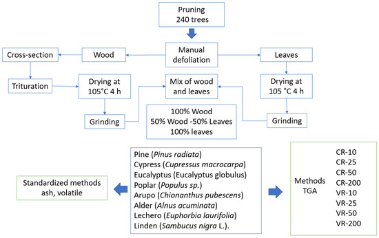
Figure 1.
Sample preparation and analysis process.

Table 1.
Heating processes were carried out on the samples that underwent thermogravimetric analysis.
To analyze the influence of the mass of the sample under analysis, samples of 15 mg, 20 mg, and 30 mg were used.
In each of the samples, the ash content was evaluated using the standardized method UNE EN ISO 18122 Solid Biofuels Determination of Ash Content and the volatile content via the standardized method UNE EN ISO 18123 Solid Biofuels Determination of Volatile Matter Content.
Regression models were obtained to identify certain points of the TGA curve defined by fixed temperatures with the standardized volatile and ash content as well as the final weight of the thermometric process.
3. Results
3.1. Assessment of the Influence of the Species
To identify whether there are significant differences between the species studied, variance analysis of the weight percentage of the non-volatilized sample subjected to the heating processes has been carried out, evaluating all the methods and compositions together at 100 °C, 175 °C, 250 °C, 325 °C, 400 °C, 450 °C, 475 °C, and 550 °C. That is, we have compared singular points of the thermogravimetric curves.
Table 2 shows that the arupo and eucalyptus species behave similarly in terms of the residual biomass of the sample at 550 °C. These form the group of species that removes the most volatiles, its residual mass being around 22.7% of the initial mass. At the opposite extreme, the group made up of the cypress and poplar samples is the one that suffers the least weight loss on heating, with a residual biomass of around 26.3%. The group formed by the species linden, pine, alder, and lechero behaves intermediately, being a transition group.
Table 2.
Analysis of variance of the weight percentage of the samples of the different species in the heating process. (Similar letters mean that there are no significant differences in each column).
It can be verified that the different species show different mass percentages at the temperatures of the heating process. It can be observed that the linden suffers a greater loss of mass in all the temperatures evaluated. However, the groups of species according to the percentage of residual mass are different at each temperature of the process. For example, linden and arupo show different behaviors at temperatures below 400 °C; however, they have the same percentage of residual mass from 400 °C. On the other hand, lechero is one of the species that releases the most volatiles below 325 °C, but its residual biomass at 550 °C is closer to the group with higher values.
Figure 2 shows the behavior of the species in the same graph, using the same method and a composition of 100% wood. As Table 1 shows, statistically, there are differences at the end of the process, but the percentages of residual masses are very similar, ranging from between 22% and 26% of the initial mass. However, it is observed that the differences are much more important at intermediate temperatures of the process, specifically between 250 and 350°C. This is due to the fact that the energy absorption for the steric translocation of the particles to be able to be released in that temperature interval is substantially different in these species.
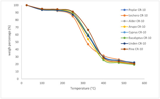
Figure 2.
Behavior of different species, subjected to a heating rate of 10 °C/minute (CR-10), with a 100% wood composition.
3.2. Evaluation of the Influence of the Heating Process
Figure 3 shows the evolution of the mass percentage with temperature in samples made up of 100% eucalyptus, poplar, lechero, and pine wood, with two different heating methods, i.e., CR-10 and CR-200.
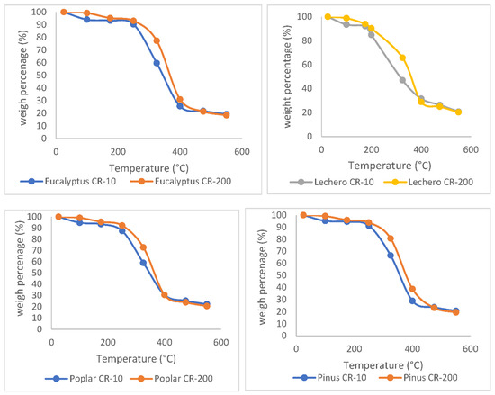
Figure 3.
Evolution of the mass percentage with temperature in samples of 100% eucalyptus, poplar, lechero, and pine wood, with two different methods, i.e., CR-10 and CR-200.
It can be seen that there is a significant variation in the curves according to the method used. In the first stage, the CR-10 and CR-200 methods cause mass loss where the dm/dT ratio is small; in the second stage, the decrease in mass increases very significantly with temperature, but unevenly; in the third stage, the decrease in mass is slowed down in such a way that at the end of the heating process at 550 °C, the percentage of residual mass is very similar in both methods, around 20%. In short, it can be deduced that at temperatures between 200 °C and 400 °C, the release of volatiles in both methods is different.
This result is very relevant, since it must be considered that the heating speed is different in both methods. In the CR-200 method, the heating rate is 200 °C/min. Therefore, the time for the experiment to reach 550 °C is 2.75 min. On the other hand, in the CR-10 method, the heating rate is 10 °C/min; so, the experiment takes 55 min. However, it is shown that the residual mass at 550° does not present great differences. This means that using the CR-200 method saves analysis time, obtaining the same results at the end of the process but different results if we consider the weights at intermediate temperatures.
Figure 4 shows the curves of all the species evaluated by these two methods on the same graph. It can be verified that, although statistically, there are differences at the end of the process, the percentages of residual masses are very similar, ranging between 19 and 23% of the initial mass. However, it is observed that the differences are much more important at intermediate temperatures of the process, specifically between 250 and 350 °C. At 325 °C, it is observed that the most pronounced differences are those found between the pine heated via the CR-200 method and the milk tree heated via the CR-10 method.
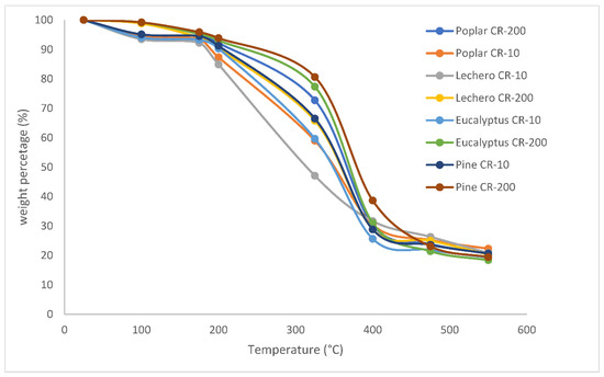
Figure 4.
Evolution of the mass percentage with temperature in samples of 100% eucalyptus, poplar, lechero, and pine wood via two different methods, i.e., CR-10 and CR-200.
Table 3 shows how the percentage of mass is influenced by the temperature and, in turn, by the heating rate of the test (Figure 4). For example, the CR-10 heating method needs 30 min of analysis to reach a temperature of 325 °C because the temperature increase is 10 °C/min, having a percentage of partial mass at that temperature of 59.7%, and the CR-200 method suffered a smaller decrease (69.2%) since it required 1.5 min of analysis.
Table 3.
Analysis of variance of the behavior of the percentage of mass depending on the method used during the tests. (Similar letters mean that there are no significant differences in each column).
It turns out that in the range from 25 °C to 325 °C there is a greater loss of mass in the methods where the sample has been heated for a longer time, compared to those that have lasted a shorter time even though they have reached the same temperature. After this interval, at the end of the experiment, a grouping of the curves is observed, which indicates homogeneous behavior, except for CR-200, which loses a greater percentage of mass with a test time of 2.63 min.
3.3. Evaluation of the Influence of the Composition on the TGA Curve
An influential factor in the volatilization during the heating process is the composition, affecting the layout of the TGA curves. Since the pruning residues used to produce chips for bioenergy are usually made up of different mixtures of wood and leaves, we proceeded to analyze how the ratio of this mixture influences the TGA curve. As can be seen in Figure 5, in the heating range between 25 °C and 150 °C, it can be observed that the samples of 100% wood composition lose a greater amount of mass as the temperature increases than the samples made up of 50% wood and 50% leaf or those formed by 100% leaf. At temperatures between 200 °C and 350 °C, the behavior of the samples is inverted, with the samples composed of 100% leaves exhibiting a greater release of volatiles, while the samples made up of 100% wood are the ones that release less volatiles (Table 4).
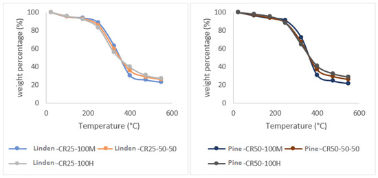
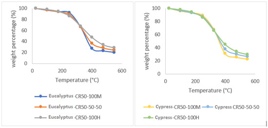
Figure 5.
Behavior of the 100% wood (100 M), 50% wood–50% leaf, and 100% leaf (100 H) compositions as a function of temperature, for cypress, eucalyptus, linden, and pine species with a heating increase of 50 °C/minute (CR-50).
Table 4.
Analysis of variance of the behavior of the mass percentage depending on the composition used during the analysis. (Similar letters mean that there are no significant differences in each column).
The residual biomass after the pyrolysis process in the samples of 100% wood comprises 21% of the initial mass; for the samples of 50% wood–50% leaves and 100% leaves, it comprises an ash residue of 25% and 28%, respectively. When the analysis is subjected to 900 °C, the 100% wood samples result in an ash content of 17% of the original mass, the 50% wood and 50% leaf sample decreases to 20% of the original mass, and for the 100% leaf specimen, the final mass is 23%. This shows that the presence of leaves alters the curve and significantly influences the plot of the curve and the final residual mass of the test. The final temperature reached is also an influencing factor.
3.4. Influence of the Final Temperature Reached
Figure 6 shows the comparison of the curves obtained to evaluate CR-25 ash and to evaluate VR-25 volatiles with an increase of 25 °C/min, for the linden, pine, cypress, and arupo species. The difference between both methods is that the final temperature of the CR-25 is 550 °C and that of the VR-25 is 900 °C. The curves obtained via both methods do not present significant differences, confirming that the residual mass of the sample in the VR-25 method is slightly lower, due to the fact that the heating process has lasted longer.
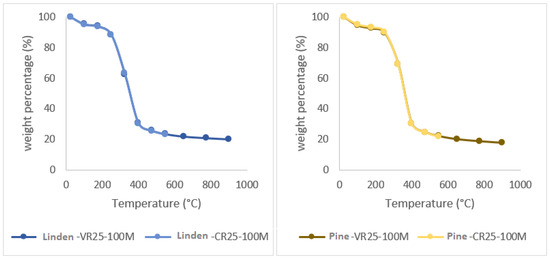
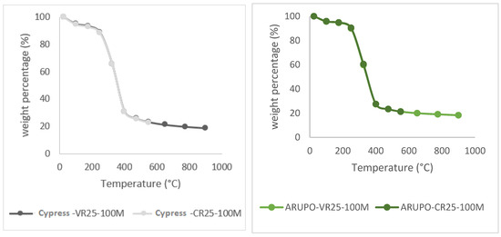
Figure 6.
Comparison of ashes and volatiles (CR-25 and VR-25), with a composition of 100% wood for the arupo, cypress, linden, and pine species.
Finally, the initial mass of the test does not affect the development of the behavior between ashes and volatiles, since there is not a great variation along the TGA, as shown in Table 5 and Figure 7.
Table 5.
Analysis of variance of the behavior of the initial mass as the temperature increases during the analysis. (Similar letters mean that there are no significant differences in each column).
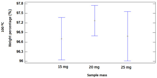
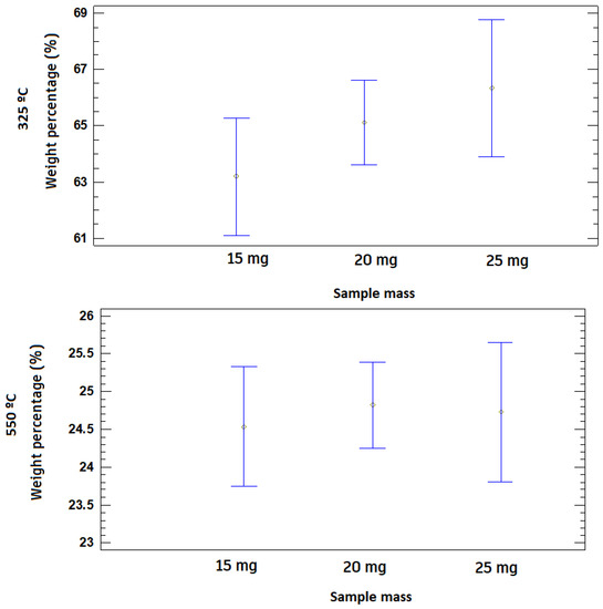
Figure 7.
LSD diagrams of the influence of the initial mass at the temperatures of 100 °C, 325 °C, and 550 °C at a 95% level of confidence.
3.5. Predictive Models of Residual Biomass, Ash, and Volatiles
As has been seen, the drawing of the thermometric curve is affected by different factors, such as the species, the composition, and the method. A scientific challenge would consist of determining mathematical models that could predict the final value of a heating process that reaches temperatures of 550 °C or 900 °C from intermediate values in the residual mass at temperatures between 100 and 300 °C. This would save time and energy.
The variation of the curves due to the influence of the factors that we have indicated shows that such a prediction would be possible and convenient. For this reason, it was evaluated as being the most appropriate method to be able to predict the residual biomass of a heating process, as well as the ash and volatile content of the sample from the residual biomass at intermediate temperatures.
Different regression models were made for each method. Table 6 shows the best heating methods for any species and composition, where Pi is the weight percentage that was not volatilized in the sample at a temperature of i °C. Table 7 shows the statistics obtained for the different regression models, which were validated with samples independent from those used to obtain the models.
Table 6.
Regression models to predict the percentage of volatiles, ash, and residual biomass in TGA and muffle.
Table 7.
Statistics of the regression models to predict the percentage of volatiles, ash, and residual biomass in TGA and muffle (Raj2 is the adjusted coefficient of determination, MAE is the mean absolute error, RMS is the root mean square, AIC is the Akaike information criterion, BIC is the Bayesian information criterion).
4. Discussion
The development of renewable energies has generated a boom in research in order to obtain a greater optimization of energy. Researchers around the world are working on elemental, proximal, structural, thermogravimetric, and fermentative analysis. The results reported in this work demonstrate several important considerations in carbonization kinetics through a thermogravimetric analysis of biomass for energy use. The kinetic study of biomass pyrolysis is relevant because it is the predecessor of combustion and gasification [10]. It should be noted that the selected samples come from the Andean province of Ecuador. Less industrialized countries obtain their main source of energy from wood, agricultural waste, and dung. From an environmental point of view, the use of biomass as an energy source should be directed towards the waste generated in different human activities. This implies the knowledge of the materials produced, which could be very heterogeneous [11,12].
The results obtained in our research are in line with the observations of Montoya [13] and Dhaundiyal and Tewari [13,14]. Four stages of mass loss can be seen: the first stage is in the temperature range of 20 °C to 120 °C; the second stage comprises 120 °C to 300 °C without a great loss of mass, where CO and CO2 are released, which come from the dehydration and decarboxylation of R-OH groups of lignin and hemicellulose; the third stage is from 300 °C to 400 °C, where the greatest weight loss occurs. At this stage, the random fragmentation of cellulose, hemicellulose, and glycosidic bonds generates volatile compounds with a high oxygen content, leaving a carbonaceous residue known as char. Finally, at temperatures above 400 °C, CO and CO2 are released through the depolymerization reactions of the lignin-rich aromatic carbonaceous matrix [15].
The loss of volatiles in the biomass goes hand in hand with temperature. According to Lin [16], the heating speed has an effect on cellulose degradation values, the kinetic model, the activation energy, and the final products [10]. The destruction of the three main components of biomass (cellulose, hemicellulose, and lignin) is the result of devolatization kinetics [17]. Cellulose and hemicellulose tend to produce the most volatiles [13]. The yield produced via pyrolysis is a function of the raw material used, temperature, heating speed, and residence time, among others.
Temperature and heating rates are the most important parameters in biomass pyrolysis. Average temperatures between 250 and 300 °C normally maximize yield. Temperatures above or below this range slow down gasification [18].
It is questionable to make generalizations of kinetic parameters when working with different heating rates and biomasses. Some authors conclude that the use of different heating rates during pyrolysis have a minimal impact on the frequency factor [19]; however, others state that biomass conversion reactions are kinetically slower at higher rates of heating [20].
Most researchers have studied thermogravimetric analysis with small temperature increases, evaluating the result when a temperature of 550 or 900 °C is reached. González et al. [21,22] used 3 °C/min, and Chenxi et al. [23] used 5 °C/min. This implies long analysis times. Long analysis times mean that it is not possible to undertake a large-scale evaluation of the waste entering a gasification or carbonization plant, which would allow the process to be adjusted and optimized.
If instead of waiting for the end of the experiment, intermediate values are taken to predict the final weight of the sample or higher temperature increases are used, we can reduce the analysis time.
Equations (1) to (7) show the calculation of the volatile and ash content allow these times to be reduced, which represents an improvement to the experiments of researchers such as Tapasvi et al. [24], who used 5 °C/min and had to spend 30 to 60 min for the test. This has led to recent research testing higher ratios as Nisar et al. [25] who used ramps of 10 °C/min, or Alsulami et al. [26] who used 10, 20, and 30 °C/min. The research carried out in our work was more ambitious.
5. Conclusions
In this work, equations are proposed that allow calculating the percentage of residual biomass that remains after a thermogravimetric analysis from the intermediate values of percentage weight with respect to the initial sample. In the same way, equations are also proposed that allow the calculation of the percentage of ash and volatiles with short analysis times. The applicability of these models has been validated in samples other than those used to obtain the models. The main finding has been the models developed for ash and volatiles determination through TGA, with time reduced to 75 s when a temperature increase of 200°C per minute is used (CR-200 and VR-200 models). To achieve the precise values of ash and volatiles in a few seconds will allow large-scale analysis in industries that receive biomass for gasification or carbonization towers. Instead of requiring hours of analysis, a precise method in a few seconds will allow the exhaustive control of the raw material in these processes.
Other additional conclusions are as follows: the species influences the release of volatiles during the heating process since, at a certain temperature, with the same method of heating, and the same percentage of wood and leaves, the behavior in the release of volatiles varies according to the species. These differences in biomass behavior in each species depend in turn on the temperature at which the comparison is made. This means that there is an interaction between the species factor and the temperature, which is obviously caused by the composition of the volatiles and the energy they require to be released.
According to the exposed thermogravimetric analyses, it is shown that the speed with which the biomass temperature increases in the TGA analysis influences the number of volatiles released in a very significant way between 150 and 400 °C. Therefore, the heating rate of the test directly influences the percentage of residual biomass in the temperature ranges below 400 °C. However, the behavior of the lignocellulosic biomass is similar at values higher than this temperature.
The mixture of wood and leaves influences both the plot of the curves and the residual biomass of the analysis. Samples of 100% wood lose a greater number of volatiles at low temperatures than samples containing higher percentages of leaf. The higher the leaf content, the greater the amount of biomass at the end of the experiment, but the latter achieves a greater release of volatiles at intermediate temperatures due to their molecular properties.
The curves obtained from the thermogravimetric analysis on the same biomass do not differ if the speed of temperature increase is similar, but they present different residual biomasses if temperatures reach 550 °C and 900 °C, since they release more gases when the final temperature is higher. Presumably, the residual biomass will reach a minimum value if the temperature reached is high enough.
Therefore, this paper demonstrates that the layout of the curve is influenced by the composition, the heating speed, and the percentage of leaves. This variability makes it necessary to select an analytical method that is as effective and as short as possible. In this article, rapid analyses combined with the application of the equations obtained are proposed.
Author Contributions
B.V.M.: performed the conceptualization, methodology, validation, formal analysis, investigation and writing—original draft preparation, writing—review and editing, and funding acquisition. J.G.-C.: performed the formal analysis and funding acquisition. I.L.C.: performed the methodology, validation. L.E.O.A.: formal analysis, investigation. All authors have read and agreed to the published version of the manuscript.
Funding
This research received no external funding.
Data Availability Statement
The datasets during the current study are available from the corresponding author on reasonable request.
Acknowledgments
This work was carried out within the framework of a study examining the analysis of the implementation of biomass exploitation chains in rural communities in the province of Bolívar (Ecuador) as part of the ADSIEO-COOPERATION program of the Polytechnic University of Valencia (UPV). The Ecuadorian Energy Exploitation Research Network of Biomass (ECUMASA) and the IBEROMASA Network of the Ibero-American Program of Science and Technology for Development (CYTED) participated in this program.
Conflicts of Interest
The authors declare no conflict of interest.
References
- Zhai, M.; Guo, L.; Zhang, Y.; Dong, P.; Qi, G.; Huang, Y. Kinetic parameters of biomass pyrolysis by TGA. BioResources 2016, 11, 8548–8557. [Google Scholar] [CrossRef]
- Skreiberg, A.; Skreiberg, Ø.; Sandquist, J.; Sørum, L. TGA and macro-TGA characterisation of biomass fuels and fuel mixtures. Fuel 2011, 90, 2182–2197. [Google Scholar] [CrossRef]
- Velázquez-Martí, B. Aprovechamiento de la Biomasa para uso Energético, 2nd ed.; Reverté: Barcelona, Spain, 2017; ISBN 978-84-9048-675-7. [Google Scholar]
- Velázquez-Martí, B.; Gaibor-Chávez, J.; Niño-Ruiz, Z.; Cortés-Rojas, E. Development of biomass fast proximate analysis by thermogravimetric scale. Renew. Energy 2018, 126, 954–959. [Google Scholar] [CrossRef]
- Gu, T.; Fu, Z.; Berning, T.; Li, X.; Yin, C. A simplified kinetic model based on a universal description for solid fuels pyrolysis: Theoretical derivation, experimental validation, and application demonstration. Energy 2021, 225, 120133. [Google Scholar] [CrossRef]
- Soria-Verdugo, A.; Morgano, M.T.; Mätzing, H.; Goos, E.; Leibold, H.; Merz, D.; Riedel, U.; Stapf, D. Comparison of wood pyrolysis kinetic data derived from thermogravimetric experiments by model-fitting and model-free methods. Energy Convers. Manag. 2020, 212, 112818. [Google Scholar] [CrossRef]
- Sebastian Arroyo-Vinueza, J.; Salvatore Reina-Guzman, W. Exploitation of biomass resources in the form of wood waste for steam boiler. INGENIUS Rev. Cienc. Tecnol. 2016, 20–29. [Google Scholar]
- Lapuerta, M.; Hernández, J.J.; Rodríguez, J. Kinetics of devolatilisation of forestry wastes from thermogravimetric analysis. Biomass Bioenergy 2004, 27, 385–391. [Google Scholar] [CrossRef]
- Mayoral, M.C.; Izquierdo, M.T.; Andrés, J.M.; Rubio, B. Different approaches to proximate analysis by thermogravimetry analysis. Thermochim. Acta 2001, 370, 91–97. [Google Scholar] [CrossRef]
- Quesada-González, O.; Cantos-Macias, M.A.; L.-Duharte, W.; Pozo-González, D.M.; Bigñot-Favier, L.C. Efecto de la velocidad de calentamiento y la biomasa en la cinética de su pirólisis. Rev. Cuba. Química 2019, 31, 478–497. [Google Scholar]
- Romero Millán, L.M.; Cruz Domínguez, M.A.; Sierra Vargas, F.E. Efecto de la temperatura en el potencial de aprovechamiento energético de los productos de la pirólisis del cuesco de palma. Tecnura 2016, 20, 89–99. [Google Scholar]
- Merdun, H.; Laougé, Z.B. Kinetic and thermodynamic analyses during co-pyrolysis of greenhouse wastes and coal by TGA. Renew. Energy 2021, 163, 453–464. [Google Scholar] [CrossRef]
- Montoya, J.I.; Chejne-Janna, F.; Garcia-Pérez, M. Fast pyrolysis of biomass: A review of relevant aspects: Part I: Parametric study. Dyna 2015, 82, 239–248. [Google Scholar] [CrossRef]
- Dhaundiyal, A.; Tewari, P. Kinetic parameters for the thermal decomposition of forest waste using distributed activation energy model (DAEM). Environ. Clim. Technol. 2017, 19, 15–32. [Google Scholar] [CrossRef]
- Cheng, F.; Zhang, X.; Yang, X.; Li, R.; Wu, Y. Research on carbonization kinetic of cellulose-based materials and its application. J. Anal. Appl. Pyrolysis 2021, 158, 105232. [Google Scholar] [CrossRef]
- Lin, Y.; Liao, Y.; Yu, Z.; Fang, S.; Ma, X. The investigation of co-combustion of sewage sludge and oil shale using thermogravimetric analysis. Thermochim. Acta 2017, 653, 71–78. [Google Scholar] [CrossRef]
- Folgueras, M.B.; Díaz, R.M.; Xiberta, J.; Prieto, I. Thermogravimetric analysis of the co-combustion of coal and sewage sludge. Fuel 2003, 82, 2051–2055. [Google Scholar] [CrossRef]
- Nurazzi, N.M.; Asyraf, M.R.M.; Rayung, M.; Norrrahim, M.N.F.; Shazleen, S.S.; Rani, M.S.A.; Shafi, A.R.; Aisyah, H.A.; Radzi, M.H.M.; Sabaruddin, F.A. Thermogravimetric analysis properties of cellulosic natural fiber polymer composites: A review on influence of chemical treatments. Polymers 2021, 13, 2710. [Google Scholar] [CrossRef] [PubMed]
- Osman, A.I.; Fawzy, S.; Farrell, C.; Ala’a, H.; Harrison, J.; Al-Mawali, S.; Rooney, D.W. Comprehensive thermokinetic modelling and predictions of cellulose decomposition in isothermal, non-isothermal, and stepwise heating modes. J. Anal. Appl. Pyrolysis 2022, 161, 105427. [Google Scholar] [CrossRef]
- Sahoo, A.; Kumar, S.; Kumar, J.; Bhaskar, T. A detailed assessment of pyrolysis kinetics of invasive lignocellulosic biomasses (Prosopis juliflora and Lantana camara) by thermogravimetric analysis. Bioresour. Technol. 2021, 319, 124060. [Google Scholar] [CrossRef] [PubMed]
- Martínez, M.G.; Dupont, C.; Thiéry, S.; Meyer, X.-M.; Gourdon, C. Impact of biomass diversity on torrefaction: Study of solid conversion and volatile species formation through an innovative TGA-GC/MS apparatus. Biomass Bioenergy 2018, 119, 43–53. [Google Scholar] [CrossRef]
- Martínez, M.G.; Couce, A.A.; Dupont, C.; da Silva Perez, D.; Thiéry, S.; Meyer, X.; Gourdon, C. Torrefaction of cellulose, hemicelluloses and lignin extracted from woody and agricultural biomass in TGA-GC/MS: Linking production profiles of volatile species to biomass type and macromolecular composition. Ind. Crops Prod. 2022, 176, 114350. [Google Scholar] [CrossRef]
- Zhao, C.; Jiang, E.; Chen, A. Volatile production from pyrolysis of cellulose, hemicellulose and lignin. J. Energy Inst. 2017, 90, 902–913. [Google Scholar] [CrossRef]
- Tapasvi, D.; Khalil, R.; Skreiberg, Ø.; Tran, K.-Q.; Grønli, M. Torrefaction of Norwegian Birch and Spruce: An Experimental Study Using Macro-TGA. Energy Fuels 2012, 26, 5232–5240. [Google Scholar] [CrossRef]
- Nisar, J.; Rahman, A.; Ali, G.; Shah, A.; Farooqi, Z.H.; Bhatti, I.A.; Iqbal, M.; Rehman, N.U. Pyrolysis of almond shells waste: Effect of zinc oxide on kinetics and product distribution. Biomass Convers. Biorefinery 2022, 12, 2583–2595. [Google Scholar] [CrossRef]
- Alsulami, R.A.; El-Sayed, S.A.; Eltaher, M.A.; Mohammad, A.; Almitani, K.H.; Mostafa, M.E. Thermal decomposition characterization and kinetic parameters estimation for date palm wastes and their blends using TGA. Fuel 2023, 334, 126600. [Google Scholar] [CrossRef]
Disclaimer/Publisher’s Note: The statements, opinions and data contained in all publications are solely those of the individual author(s) and contributor(s) and not of MDPI and/or the editor(s). MDPI and/or the editor(s) disclaim responsibility for any injury to people or property resulting from any ideas, methods, instructions or products referred to in the content. |
© 2023 by the authors. Licensee MDPI, Basel, Switzerland. This article is an open access article distributed under the terms and conditions of the Creative Commons Attribution (CC BY) license (https://creativecommons.org/licenses/by/4.0/).