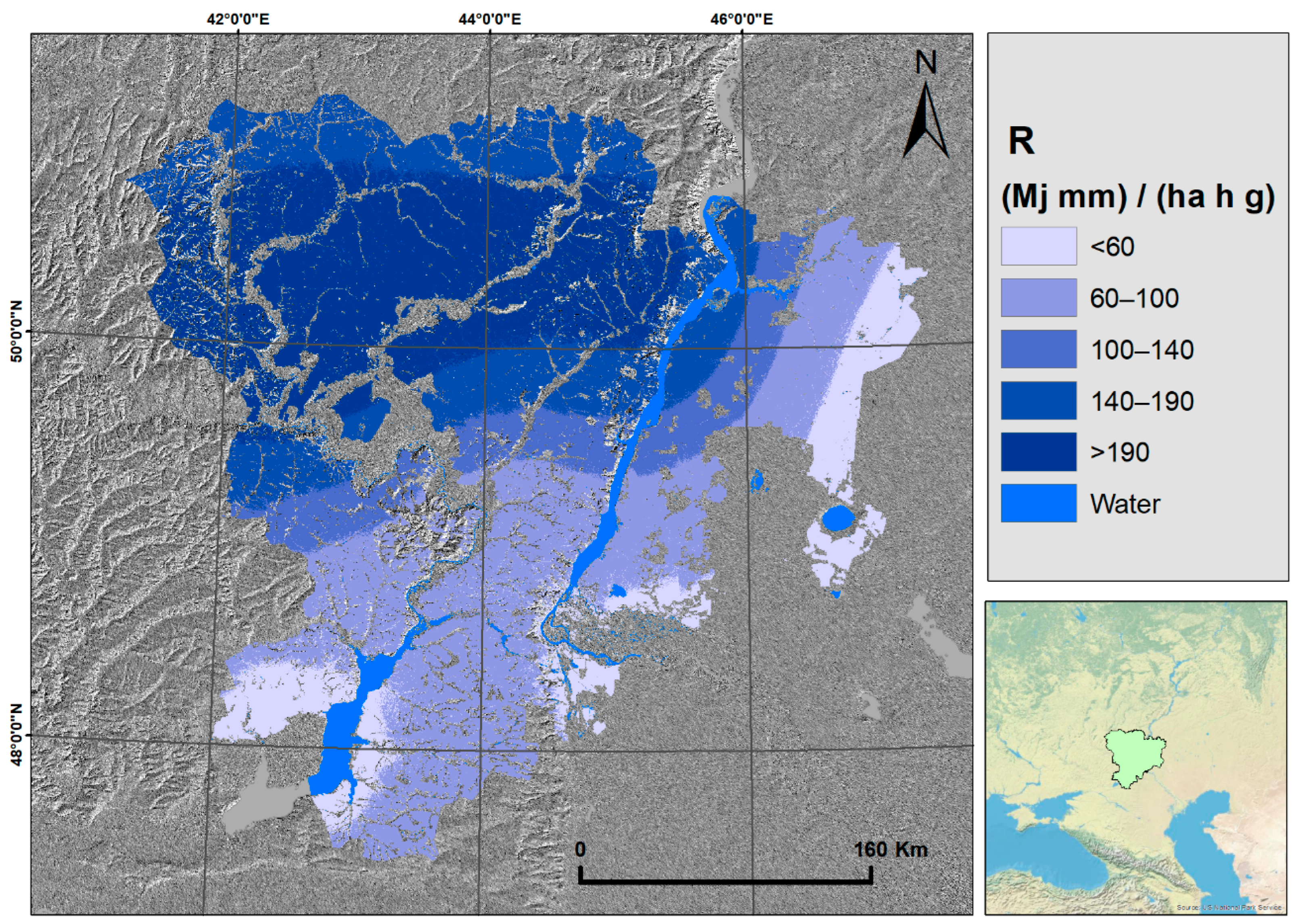
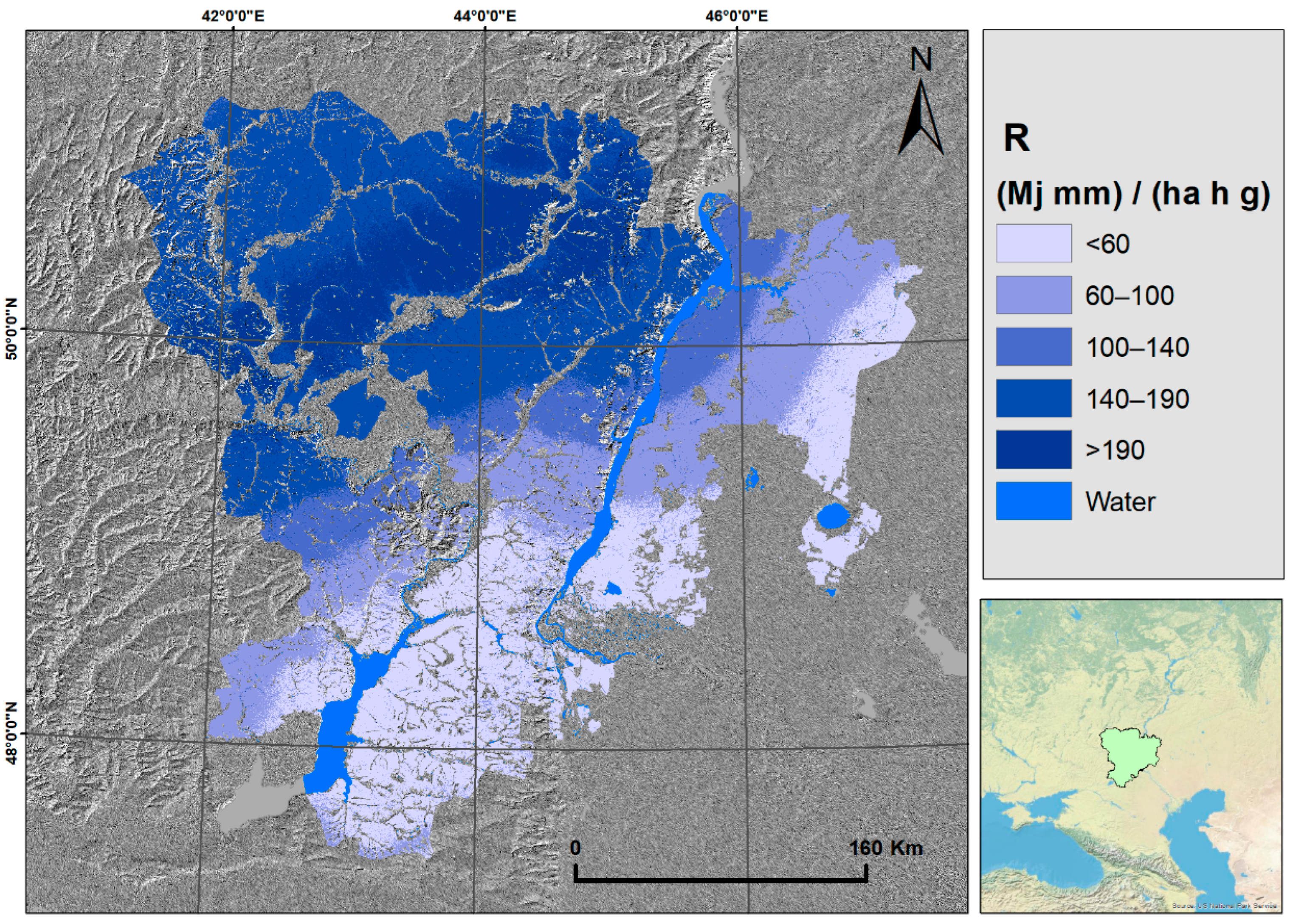
Article

Modeling Dynamics of Soil Erosion by Water Due to Soil Organic Matter Change (1980–2020) in the Steppe Zone of Russia

by
Nikita R. Kriuchkov
1,2,* and
Oleg A. Makarov
3
1
Faculty of Biology, Shenzhen MSU-BIT University, International University Park Road 1, Dayun New Town, Longgang District, Shenzhen 517182, China
2
Department of General Ecology and Hydrobiology, Faculty of Biology, Lomonosov Moscow State University, 119991 Moscow, Russia
3
Department of Soil Erosion and Soil Conservation, Faculty of Soil Science, Lomonosov Moscow State University, 119991 Moscow, Russia
*
Author to whom correspondence should be addressed.
Agronomy 2023, 13(10), 2527; https://doi.org/10.3390/agronomy13102527
Submission received: 15 August 2023 / Revised: 25 September 2023 / Accepted: 27 September 2023 / Published: 29 September 2023

Abstract

:
This research aims to evaluate the dynamics of soil loss through soil erosion by water in agricultural lands in steppe areas using a modification of the RUSLE2 model from the 1980s to the 2010s. The calculation was performed using a raster model of data that included a model of the slope angle, slope length, soil erodibility, rainfall and snowmelt erosivity factors, types of land use, and cover management factor. All data were taken from open sources. The average soil erosion in the territory studied amounted to 1.48 t ha−1 year−1 in the 1980s and 1.72 t ha−1 year−1 in the 2010s. The discrepancy with other studies was 12% for the level of the 1980s and 2–7% for the level of the 2010s. The main factor leading to an increase in soil loss was soil erodibility due to the loss of soil organic matter, which affected about 52% of the studied lands. The increase in the amount of soil loss occurred against a background of compensating processes: reduction in precipitation and climate change (getting drier), as well as the overgrowth of agricultural lands with natural steppe vegetation. Modified model RUSLE2 has shown good results correlated with other studies for the research area.

1. Introduction

Water is an essential natural resource for sustaining life on Earth, but its unchecked movement and excessive flow can also have devastating consequences. One of the most significant impacts of water on the environment is soil erosion by water, which is the process of soil and rock being worn away by the force of water [1]. Soil erosion by water has been a natural process throughout the Earth’s history, but human activities such as deforestation, intensive agriculture, and urbanization have accelerated this process, causing severe environmental problems [2]. The adverse effects of soil erosion by water on the environment include a loss of soil fertility, reduced crop yields, sedimentation in water bodies, and the destruction of habitats [3,4,5,6,7]. Furthermore, soil erosion by water constitutes one of the most potent processes of soil and land degradation, resulting in the degradation of the quality of ecosystem services provided. These services hold significance not only for human populations but also for the entire biocenosis [2,8]. Therefore, understanding the mechanisms and impacts of soil erosion by water is critical for developing effective strategies to mitigate its effects and protect our environment [9].
With the increasing effects of climate change, soil erosion by water has become an even more pressing issue. Rising temperatures, altered precipitation patterns, and more frequent extreme weather events can exacerbate erosion rates and intensify the damage caused by erosion [7]. Climate change can affect erosion processes in various ways, such as by altering the amount, intensity, and frequency of rainfall and modifying the vegetation cover and the topography of landscapes. These changes can increase erosion rates, cause soil loss, and reduce agricultural land productivity [10]. Furthermore, the impacts of climate change-induced erosion are not limited to specific regions or countries but have global implications, as the sediment and pollutants carried by eroding water can travel long distances and affect ecosystems far from the source [10]. To mitigate the impacts of soil erosion by water in the context of climate change, it is crucial to understand the underlying processes, assess the vulnerability of different regions and landscapes, and develop appropriate management strategies [2,11].
Arid lands are vulnerable zones in climate change [12,13]. The combination of low vegetation cover, high soil erodibility and erratic rainfall makes arid lands particularly prone to erosion. Even small amounts of rainfall can cause significant soil loss and degradation [14,15]. It is fascinating to understand how climate changes affect soil erosion. On the one hand, the precipitation decreases, leading to decreased soil losses due to rain. On the other hand, the number of extreme weather events increases, which can lead to an increase in soil losses due to short rainfall but high kinetic energy phenomena. Under the latest Intergovernmental Panel on Climate Change (IPCC) Report [16], there has been a discernible upward trend in the frequency of intense precipitation events observed since the 1950s across numerous geographical regions, including the specific research site under consideration. Furthermore, the report posits a likelihood of further exacerbation in the incidence of heavy precipitation events in the foreseeable future [16,17,18].
This research represents a pioneering effort in the high-resolution spatial modeling of soil erosion by water in steppe areas considering national dynamics (the 1980s to 2010s) in Russia. To our knowledge, this study is the first to comprehensively investigate the dynamics of soil erosion by water processes, utilizing advanced modeling techniques and incorporating detailed spatial data. Other papers focused on a large-scale current level of soil erosion by water [3,19,20,21,22] or provided data for the last century without spatial distribution [19,23,24]. By addressing this critical knowledge gap, our work aims to significantly contribute to understanding erosion patterns and distribution and provide valuable insights for sustainable land management and conservation efforts in the steppe regions of Russia.
The primary objective of this study was to comprehensively assess the dynamics of soil erosion by water over the past four decades (from 1980 to 2020) within the steppe zone of the Volgograd region, Russia. Specifically, our research sought to investigate the influence of climate variability and change on the regional-scale water erosion patterns. This endeavor was motivated by the imperative to gain a deeper understanding of the intricate interplay between climate fluctuations and their impact on the levels of water-induced erosion, which is vital for informed land management and conservation strategies in the region.

2. Materials and Methods

2.1. Research Area

The Volgograd region, Russia is located in the southeast of the East European Plain and is the most significant region in the south of Russia. The region’s relief is diverse—from a lowland plain in the Volga region in the east to an elevated dismembered territory in the north and west. The DEM and Slope maps are shown in Figure 1 and Figure 2.
The climate of the region is arid, with pronounced continentality. The north-western part is located in the forest–steppe zone, the central and south are in the steppe zone, and the eastern part is in the semi-desert zone, approaching real deserts [25]. The map of land use according to Chen and co-authors [26] is shown in Figure 3.
The study area exhibits distinct climatic gradients, with average annual precipitation ranging from approximately 500 mm in the northwest to less than 300 mm in the southeast. Moreover, extreme climatic conditions are observed, including absolute maximum temperatures of +42 °C to +44 °C typically occurring during July and August, while absolute minimum air temperatures plummet to −36 °C to −42 °C in the winter months of January and February [25].
The region is located within two soil zones—chernozem and kastanozems. The soil and texture maps are shown in Figure 4 and Figure 5.
The total square area of agricultural land is 76,100 km2. The total population of people—2,492,808. The share of urban residents is 77%. The people density is 21.87 people/km2 [25].

2.2. The Technique for Calculating Potential Soil Erosion

We used the RUSLE2 [27] model as a basis to carry out the simulation. However, we approached the choice of the formula for calculating its indicators by considering the available data and the characteristics of the object of study. For example, the RUSLE-2 model needs to work better on soils with a high organic matter content (>4%), which are widespread in the Volgograd region [25,27,28]. Because of this, we applied a different algorithm for calculating the K-factor, taking into account the features of the object. In the case of calculating the R-factor, the problem was the absence of pluviographs at most meteorological stations in the region. Furthermore, standard precipitation data are published as the sum of precipitation for 3 h (180 min), which makes it impossible to apply the formula for calculating the R-factor for precipitation that fell in 60 min or less according to the formula laid down in the model.
Two periods were chosen for modeling to assess the dynamics of soil erosion by water—the level of the 1980s and the level of the 2010s. All model calculations for the research area were performed in raster layers with 30 m resolution (Figure 6).
(1)
Model calculations were performed as follows:
(2)
Collecting data for calculating factors of soil erosion.
(3)
Choosing optimal model parameters for performing calculations.
(4)
Modelling of soil erosion.
(5)
Checking the quality of results with other research.

2.3. Rainfall and Snowmelt Erosivity Factors

Data from the meteorological station of the Roshydromet network located in the Volgograd region were used to calculate the R-factor. The data were provided by RIHMI-WDC [29]. Data were separated into two ranges: 1970–1998 (Rainfall erosivity in the 1980s) and 1999–2019 (Rainfall erosivity in the 2010s).
The R-factor was calculated according to the approach proposed by Naipal [30]. The formula for calculating the R-factor varies depending on the type of climate (according to Köppen). Data on the distribution of climate types by Köppen in the Volgograd region were taken from the article by Peel et al. [31].
For area with «Hot-summer humid continental climate (Dfa)», we used Formula (1)
ln R = 1.99 + 0.737 × ln P + 2.033 × ln S D I I ,      
For area with «Warm-summer humid continental climate (Dfb)», we used Formula (2):
ln R = 0.5 + 0.266 × ln P + 3.1 × ln S D I I 0.131 × ln Z ,
Values of variables: ln R—the natural logarithm of the R-factor; ln P—the natural logarithm of the average annual precipitation; and ln SDII—the natural logarithm of the precipitation intensity index. SDII is calculated as the ratio of precipitation per year to the number of days per year with precipitation >1 mm; ln Z is the natural logarithm of the height of the location of the meteorological station.
The amount of snowmelt runoff was calculated by multiplying the precipitation that fell from December to March by a coefficient of 0.0591 [32]. After the calculation, this value was added to the amount of stormwater runoff.

2.4. Soil Erodibility Factor

As is well known, the RUSLE model works poorly with soils with content of SOM > 4% [27,28,33]. In our case, 65% of the research area had chernozem and kastanozem soils with a high SOM content. Because of this, we used a modern step-by-step approach for soil erodibility calculation presented in an article by Auerswald and co-authors [28].
Algorithm based on step-by-step calculations. Choosing an equation depends on the condition. All Equations (3)–(10) are below:
K 1 = 2.77 × 10 5 × ( f s i + v f s a × 100 f c l ) 1.14    
K 1 = 1.75 × 10 5 × ( f s i + v f s a × 100 f c l ) 1.14   + 0.0024 × f s i + v f s a + 0.16
K 2 = 12 f o m / 10  
K 2 = 0.8
K 3 = K 1   × K 2   + 0.043 × A 2 + 0.033 × P 3
K 3 = 0.091 0.34 × K 1   × K 2   + 1.79 × K 1   × K 2   2 + 0.24 × K 1   × K 2   × A + 0.033 × P 3
K   = K 3  
K = K 3 × ( 1.1 × e x p ( 0.024 × f r f ) 0.06 )
If f s i + v f s a (mass fraction (in %) of silt plus very fine sand) less than 70%, you must use Equation (3). If not—Equation (4). If f o m (mass fraction (in %) of organic matter in the fine earth fraction) less than 4%, you must use Equation (5). If not—Equation (6).
After that, If K 1   × K 2 more than 0.2, you must use Equation (7). If not—Equation (8). If   f r f   (the fraction of the soil surface covered with rock fragments) less than 1.5%, you must use Equation (9). If not—Equation (10). f c l —mass fraction (in %) of clay in the fine earth fraction. A—soil structure index (1…4). P—permeability index (1…6) increasing from rapid to very slow.
Soil structure and soil permeability were defined according to Panagos and co-authors [34]. The algorithm is presented in Table 1 and Table 2.
For the calculation of soil erodibility in the 2010s, we used open-source data. The list of sources is below:
  • The Red Book of soils of the Volgograd region [25].
  • Unified State Register of Soil Recourses of Russia [35].
  • Our data, collected in 2019 [36].
To calculate soil erodibility in the 1980s, we used the ‘Soil map of Volgograd region’ in scale 1:400,000 [37]. We calculated the average K-factor based on the data used for preparing this map for each kind of soil type on this map [38].

2.5. Length Slope Factor

The LS-factor was estimated based on the Digital Elevation Model (DEM) with a 30 m resolution [39]. This DEM is a data product of the Shuttle Radar Topography Mission (SRTM) [40]. The DEM was processed according to the method proposed by L. Wang and H. Liu [41]. This method efficiently identifies the topographic lows, overland flow paths, and watershed subdivision levels, which is convenient for the LS calculation. The calculation was performed using SAGA [42]. The LS-factor of the area under study was mapped using ArcGIS 10.4.1 software.
After the processing, the LS-factor was calculated using the formula proposed by Desmet and Govers [43], Equation (11):
L ij = ( ( A i j i n + D 2 ) m + 1 A i j i n m + 1 D m + 2 x i j m 22.13 m ) m
where Aij-in is the contributing area at the inlet of the grid cell (i,j) measured in m2, D is the grid cell size (meters), Xi,j = sin aaii,jj + cos aaii,jj and the aaii,jj is the aspect direction of the grid cell (i,j).
m is related to the ratio β of the rill to interill erosion (Equation (12)):
m = β β + 1
where β (Equation (13)):
β = s i n θ 0.0896 [ 0.56 + 3 sin θ 0.8 ]
The S-factor is calculated using the Formulas (14) and (15) proposed by Renard [27]:
S = 10.8 × s i n θ + 0.03 ,   w h e r e   s l o p e   g r a d i e n t < 0.09
S = 16.8 × s i n θ 0.5 ,   w h e r e   s l o p e   g r a d i e n t 0.09

2.6. Land Use and Crop Factors

The GLOBAL LAND 30 model with a spatial resolution of 30 m was used to determine agricultural land [26]. Due to the lack of data on the contour of agricultural land during the USSR, we used the same model for data from the 1980s.
To calculate the C-factor, we took Landsat data. Landsat scenes were taken to the territory of the Volgograd region during the main vegetation period (from May to September). In order to avoid the impact of atmospheric phenomena on the quality of images, only images subjected to atmospheric correction (L2A level product) were used. The images were taken annually from 1984 to 1988 (5 years) and from 2017 to 2021 (5 years). For each year, the scenes were stitched into a single raster, and the value of the C-factor was calculated. Next, the average value of the C-factor was calculated for each of the 5-year periods.
The C-factor was calculated according to the Equation (16) suggested by Almagro et al. [44]:
C = 0.1 × N D V I + 1 2 ,
The values of the P-factor were assumed to be equal to 1.

2.7. Data Interpolation

In this paper, Empirical Bayesian Regression Kriging (EBRK) was used to set up local spatial models of the R-factor (1980s and 2010s) and K-factor (only 2010s). Two proxy variables, DEM and LS-factor, were used for the R-factor, and for the K-factor four proxy variables were used: LS-factor, DEM, soil types and a texture map of the Volgograd region.
EBRK is an interpolation technique that combines Ordinary Least Square regression and simple kriging to accurately predict moderately non-stationary data at a local scale [45]. To improve the accuracy of ordinary kriging and account for uncertainty introduced in the variogram, EBRK estimates the semivariogram through subsetting and repeated simulations. This approach is particularly beneficial for small datasets and provides better accuracy than other kriging methods [46]. EBRK also offers the advantage of reducing the smoothing effect of spatial interpolation, allowing for more precise predictions of moderately non-stationary data. Basically, the EBKR is decomposed as follows Equation (17):
y s = μ s + w s + ε ( s )
where μ   s is the mean structure to model a large-scale spatial trend in the random field (RF), w(s) is a Gaussian process GP (0, C (s1, s2; σ2, φ)) and ε(s) is Gaussian white noise N (0, τ2). The mean structure μ   x is explained by a set of covariates; μ   s = xt(s) β, where x is a vector of covariates values at location s and β is the coefficients for the covariates. Denote the model parameters as θ = {β, σ2, φ, τ2}, with σ2 representing spatial variance and φ controlling spatial decay effects. C (s1, s2) is correlation function, which provides a way to characterize spatial dependence between pairs of locations (s1, s2) [47].
The interpolation’s quality control was performed using cross-validation, which involves removing one data point to evaluate the interpolation model’s fit. This method uses the remaining data points to interpolate at the removed point’s location and then compares the interpolated value with the measured value to determine the interpolation’s accuracy. This approach is advantageous compared to other cross-validation methods because it evaluates the data against the full distribution rather than only predicting a specific point. Statistics like the root mean standard error (RMSE) and average CRPS (continuously ranked probability score) were used to assess accuracy. The average CRPS measures the deviation from all data points and predicts cumulative distribution function, and a smaller value indicates better accuracy [48]. The CRPS is decomposed as follows Equation (18):
C R P S ( F , x ) = ( F y 1 y x ) 2 dy
X is a variable. F is the cumulative distribution function (CDF) of X, such as F(y) = P[X ≤ y]. x is the observation, and F is the CDF associated with the probabilistic forecast [49].
All calculations were performed with the ArcGIS PRO 2.9.2 program. The ArcMap 10.8 program was used to prepare the cartographic material.

3. Results and Discussion

3.1. R-Factor

The Figures show the distribution maps of the R-factor on the territory of the Volgograd region in the 1980s (Figure 7) and 2010s (Figure 8).
The results of the R-factor for two range computations are presented in Table 3. The percentage distribution by classes of R-factor values is presented in Table 4.
The average value of the R-factor in the territory decreased by 9% compared to the level of the 1980s (Table 5). The share of precipitation with a low erosion potential increased, and with a high one decreased (Table 6). This fact is evident in the southern part of the region: in the territories where R-factor values were previously recorded in the range of 60–100 Mj·mm/ha·h·g, today values with R-factor <60 Mj·mm/ha·h·g are recorded (Figure 2 and Figure 3). In the north of the region, there was also a “displacement” of the erosion zone with an R-factor >190 Mj·mm/ha·h·g to a less dangerous zone with a value of 140–190 Mj·mm/ha·h·g (Figure 2 and Figure 3, Table 6).
However, the standard deviation of the R-factor increased from 64.70 in the 1980s to 74.71 in the 2010s, indicating more significant variability in the R-factor during the more recent period.
The RMSE and CRPS are measures of model accuracy, with lower values indicating a better fit to the data. The lower values in the 1980s suggest that the model performed better in that period than in the 2010s.

3.2. LS-Factor

The distribution map of the LS-factor in the Volgograd Region is shown in Figure 9.
Statistical characteristics of LS-factor values on the territory of the Volgograd region, as well as the percentage distribution by class, are given in Table 5 and Table 6.
The minimum and maximum values of the LS-factor were significantly lower or higher than average, but their total percentage value was the same (2.68% and 1.93%).
The average LS value of 0.52 is a measure of the central tendency of the dataset (66%), indicating that most points in the dataset have an LS-factor value around this value. However, as the standard deviation of 2.20 indicates, the dataset also has considerable variation.

3.3. C-Factor

Figure 10 and Figure 11 show maps of the distribution of the C-factor in the Volgograd region.
Statistical characteristics of the values of the C-factor in the Volgograd region, as well as the percentage distribution by class, are given in Table 7 and Table 8.

3.4. K-Factor

The figures show the distribution maps of the K-factor on the territory of the Volgograd region in the 1980s (Figure 12) and 2010s (Figure 13). The statistical characteristics of the K-factor values and the percentage distribution by class are given in Table 9 and Table 10.

3.5. Soil Erosion by Water

Figure 14 and Figure 15 show maps of the distribution of soil erosion levels in the territory of the Volgograd region. Figure 16 shows a map of the difference in soil loss between the 1980s and 2010s.
Statistical characteristics of the values of the amount of soil loss in the territory of the Volgograd region and the percentage distribution by class are given in Table 11 and Table 12.
The obtained data on soil loss by water erosion represent typical values for this region, averaging approximately 2 tons per hectare per year. This can be attributed to the continental climate of the area, characterized by limited precipitation, as well as the flat topography of the terrain [3,20].

3.6. Accuracy of the Results of the Calculation of Soil Erosion

To verify the results obtained, they were compared with the results of another independent research work.
We compared our results with the results from applying the soil erosion model developed under the guidance of G. A. Larionov [50]. This model was used for different regions of the European part of the Russian Federation in the work of L.F. Litvin and co-authors [23] and for the assessment of soil loss by soil erosion by water in small river basins in the work of Maltsev and Yermolaev [20]. In addition, the results were compared with those presented by Golosov with co-authors (Golosov et al., 2018 [19]). In this work, modified versions of the USLE and SHI erosion models were used for the evaluation mean annual erosion rate for 1986–2012. Only in the work of Litvin and co-authors were results for the regions presented which we could thoroughly compare with our data. The paper by Yermolaev and Maltsev provides data for the current level but by biomes. In the work of Golosov and co-authors, data are given for both the level of the 80s and 2012, but by natural zones. Therefore, we compared the results presented in the work of Maltsev and co-authors with the current value of the soil loss and the results of Golosov and co-authors to the value of the washout of the 1980s to the level of the 2010s. Results are presented in Table 13.
According to Litvin’s data [23] soil loss increased by 23.4% compared to the 1980s. We calculated the annual soil loss from the Litvin data for our area. The difference between the total area was because no USSR land use spatial data exist. Therefore, we used actual land use data for the USSR time (Methodology). The discrepancy with Litvin’s results for 1980s level data was 12%, which is extremely small and indicates a good reproducibility and reliability of the results.
The discrepancy with Litvin’s data was only 7.2%, demonstrating the high reproducibility and reliability of the data obtained. The discrepancy for the current level with Golosov and co-author’s data was less than Litvin’s and only 2.5%. But these data were not only produced for the steppe area in the Volgograd region, and represented the entire steppe area in the European plane.
Additionally, we compared our results with the results of local field erosion stations [51,52]. The results are presented in Table 14.
As can be seen from the data obtained, the difference between the field measurements and our results was not critical and ranges from 6 to 15%.
Also, a comparison was made between the Volgograd region’s erosive soil loss map and European Russia’s soil erosion map, created using the same calculation methods [20]. According to the map, erosive soil losses for the Volgograd region were 0–5 t ha−1 year−1. These values are not very different from ours, obtained here (2 t ha−1 year−1). Unfortunately, the authors did not published results by regions, only data according to natural zones. The Steppe zone is much broader than the Volgograd region and includes some parts of different areas. However, the results match if compared in the range between several zones presented in the Volgograd region. Semi-desert and steppe areas had mean 2 t ha−1 year−1 soil losses, and in our research we had 2 t ha−1 year−1.
In addition, we compared our results with the soil erosion map of the European Union [21]. A close country in landscape and climate conditions is Poland. Poland’s mean soil loss in arable land is 1.61 t ha−1 year−1. The difference between our data was 7%.

3.7. Discussion and Perspectives

The average R-factor in the Volgograd region has decreased in recent decades, and there has been more significant variability in the R-factor during the more recent period.
The R-factor depends directly on the amount of precipitation. Therefore, its decrease can be explained by a reduction in precipitation and the development of the aridification process. The results of other independent studies confirm the development of this process; for example, the work of Zolotokrylin and co-authors [53]. The authors of this work analyzed the dynamics of the Standardized Precipitation Index (SPI) for several southern regions of Russia, including the Volgograd region. It was shown that from 1970 to 2000, a wetter humidification period was observed in the region’s territory. Since 2001, it has been replaced by more arid conditions.
Another paper that has confirmed that fact is the article by Eltsov and co-authors [54]. In this paper, based on the analysis of climatic and meteorological data for the last 60 years, the authors demonstrated an increase in the aridity of the climate of the Lower Volga region and a shift in the isolines of the aridity index values (according to De Morton—IDM) of the region by about 100 km to the northwest, which also correlates with our data.
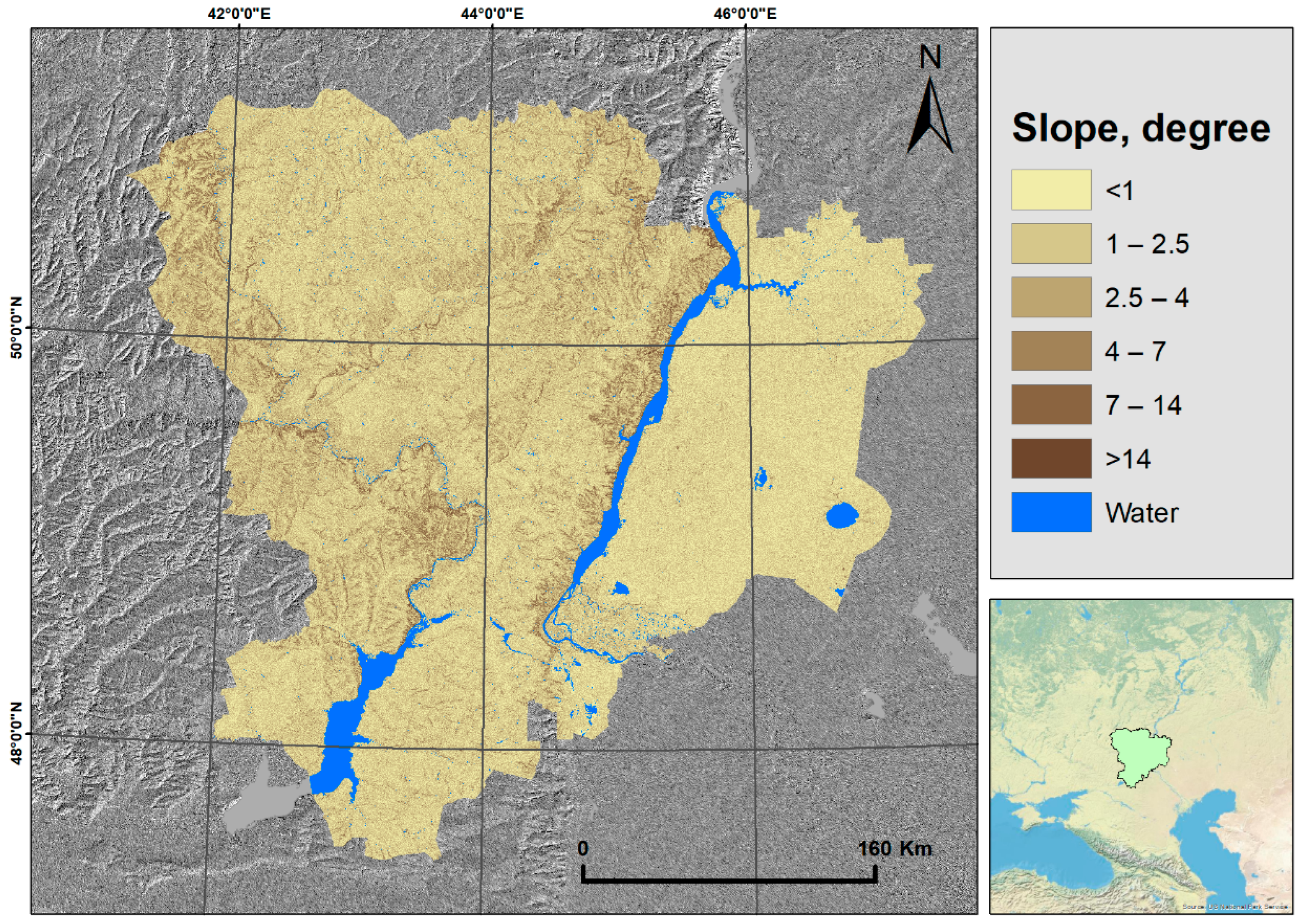
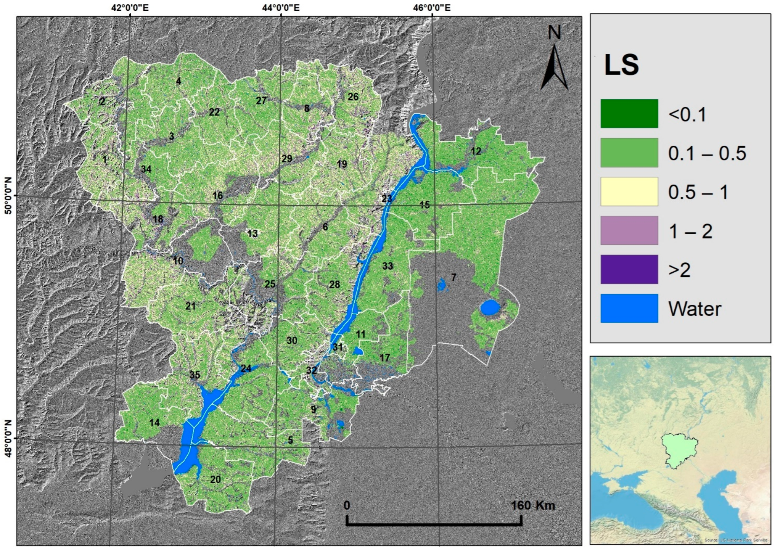
The high values of the LS-factor in the Volgograd region were associated with elevated forms of relief and, accordingly, with a higher steepness of the slopes. The main erosion-hazardous areas are the slopes of the right bank of the Volga and Don rivers. A similar pattern was observed with low values of the LS-factor, which were recorded in the region’s territories with low relief forms (the territory of the left banks of the above rivers). The highest values of the LS-factor were observed in the territory of districts, a significant part of the area of which are hills: the southeastern part of the Central Russian Upland (Alekseevsky (No. 34) and Kumylzhensky (No. 18) municipal districts) and the southern part of the Volga Upland (Kamyshinsky (No. 23) and Danilovsky (No. 29) municipal districts) (Figure 4). The lowest value of the LS-factor was recorded in territories with predominantly low-lying terrain—Sredneakhtubinsky (No. 11), Pallasovsky (No. 7), and Nikolaevsky (No. 15) municipal districts. Approximately 8% of the region’s total agricultural land is dangerous for agriculture (LS-factor > 1).
The values of the LS-factor calculated for the Volgograd Region were in good agreement with the results of similar studies performed for EU countries with predominantly flat territory—Poland, Hungary, Estonia, Netherlands, Latvia, Lithuania, and Denmark [55]. The average values of the LS-factor for the territories of these countries were 0.52, 0.59, 0.32, 0.19, 0.39, 0.35, and 0.32, respectively.
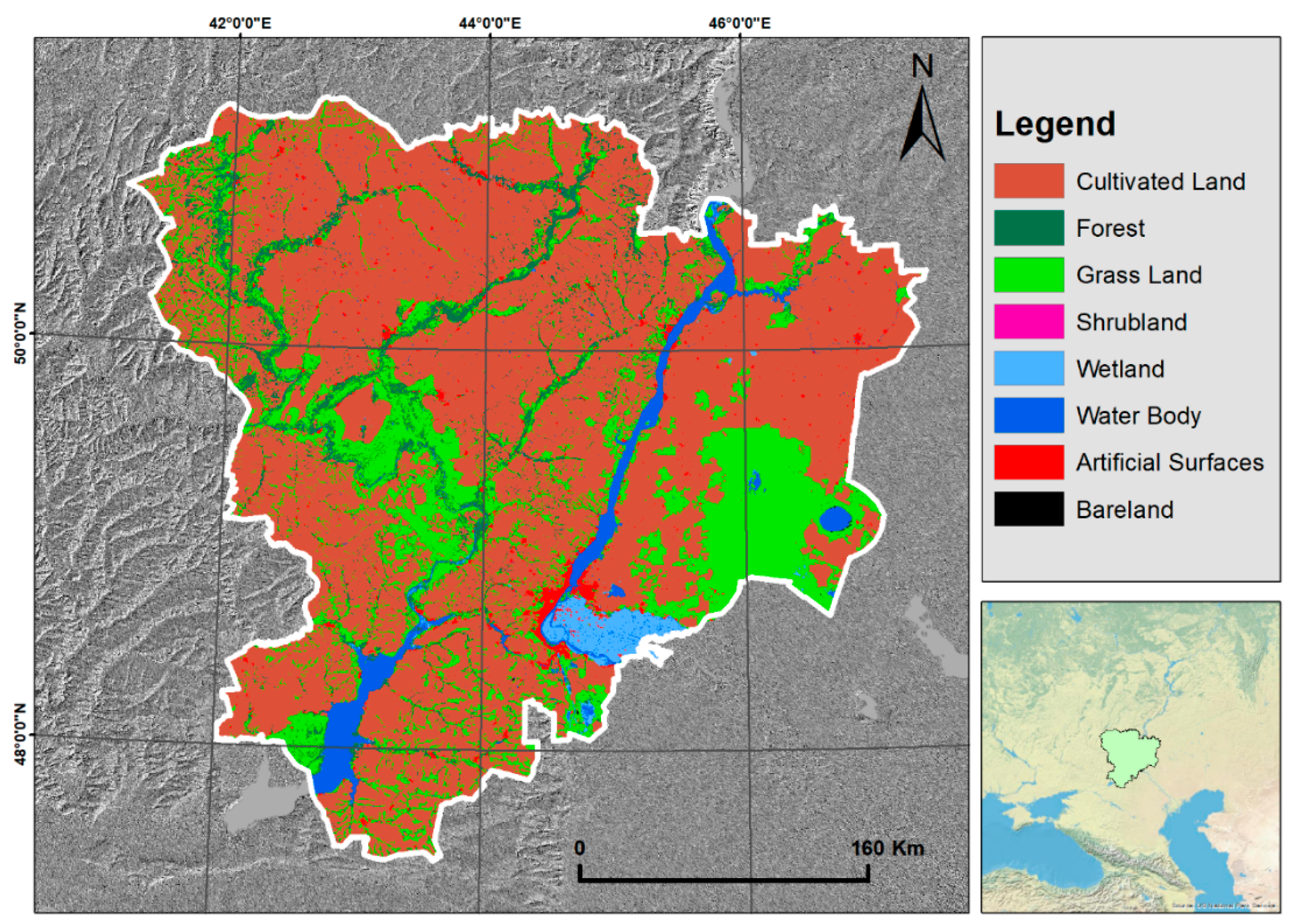
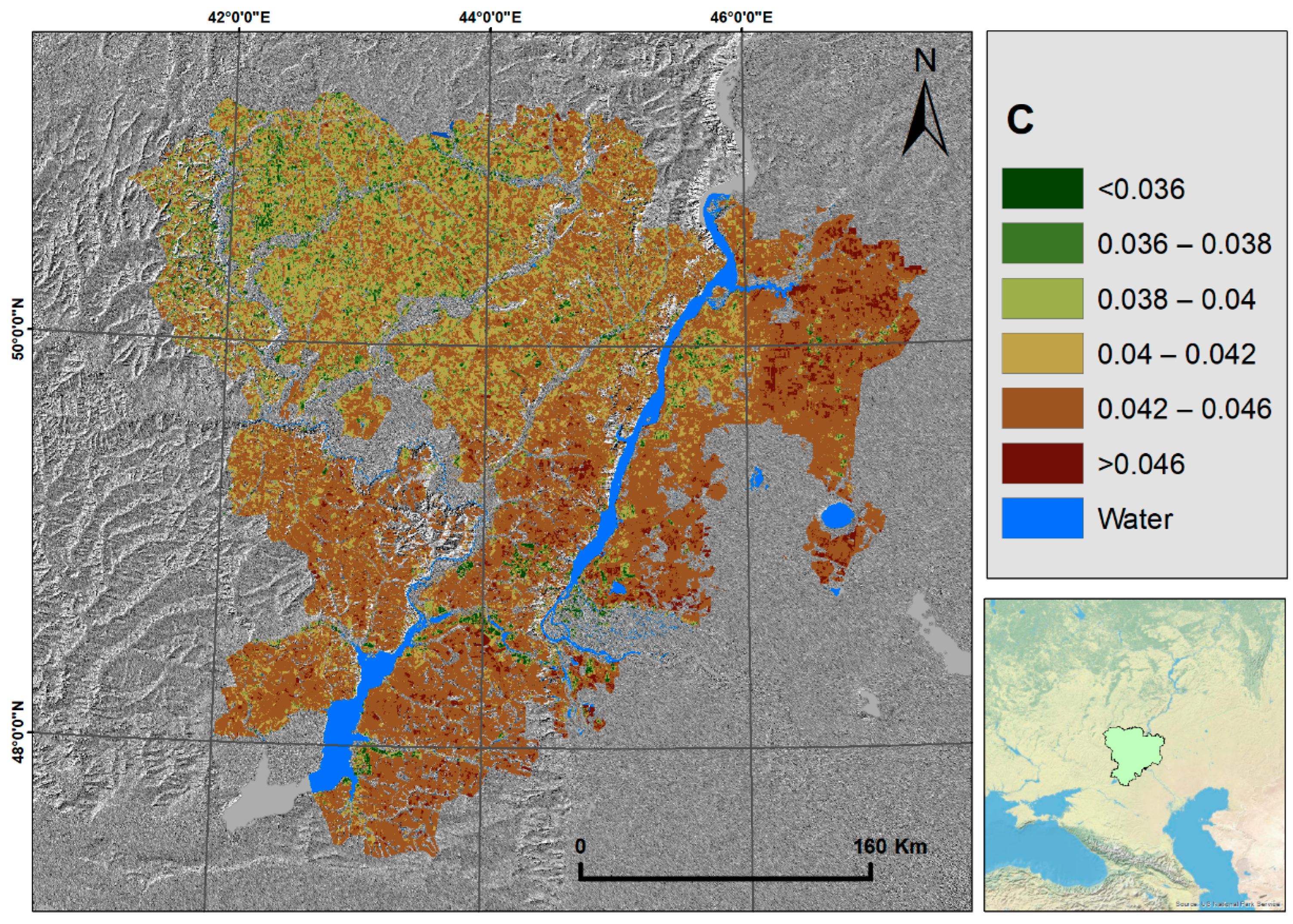
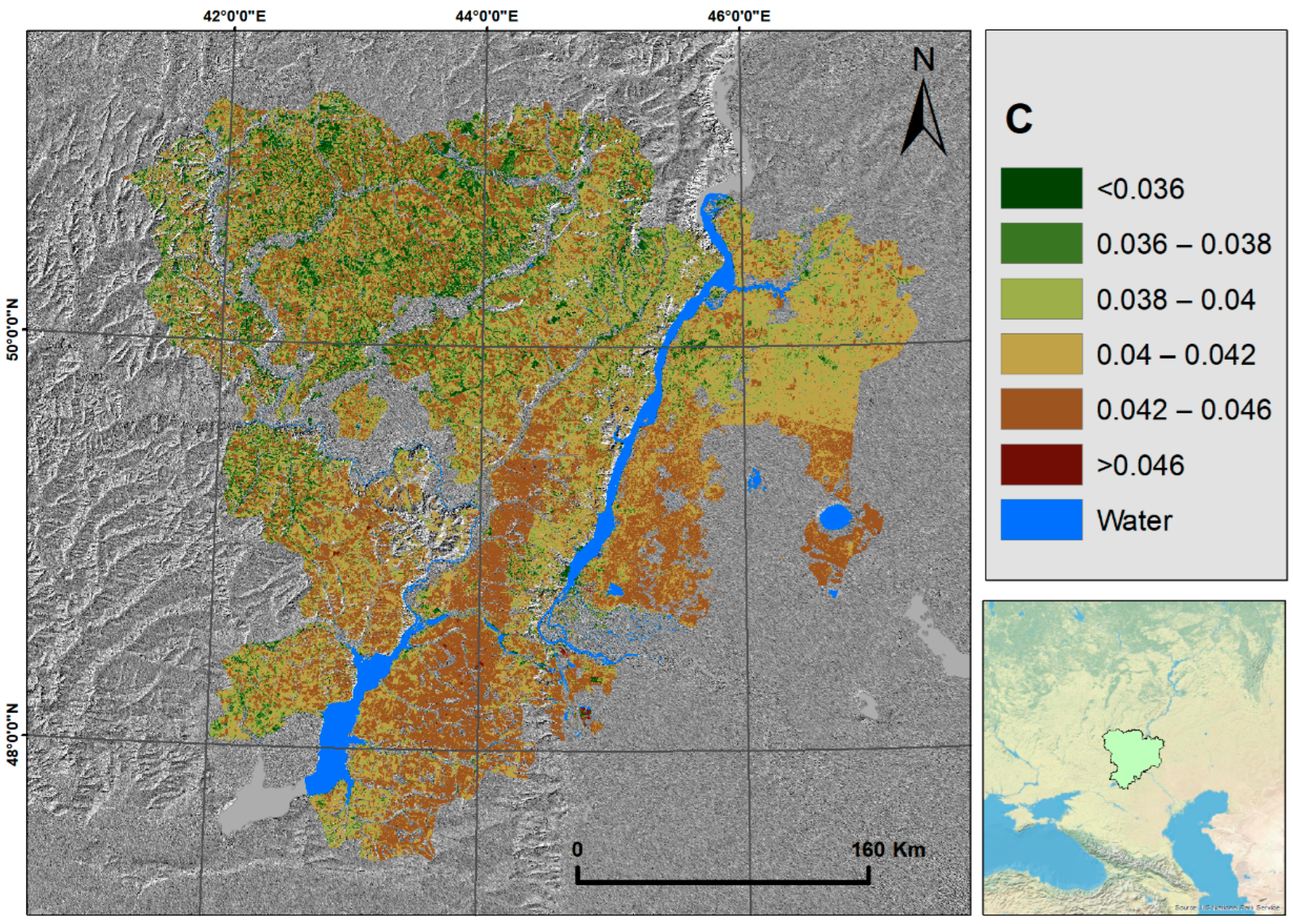
The area of contours with a high protective potential has increased, while that with a low one has fallen (Table 10). The indicator of the C-factor in the region’s territory decreased by approximately 6% compared to the level of the 1980s (Table 9). That means that the protective capacity of vegetation in the region increased by 6%. Most likely, this is due to the overgrowth of agricultural land with natural vegetation, which increased the protective degree of vegetation cover. Natural steppe vegetation has a higher erosion resistance than field crops [50]. It is worth noting that all this is happening against the background of a decrease in the amount of incoming moisture, both from natural sources (Section 3.1) and artificial ones. According to the data from Gorokhova and co-authors and Pankova and Novikova [56,57] the amount of irrigated land in the Volgograd region has decreased relative to the level of the 1980s. The value of the C-factor in the region increased from north to south and from west to east, which is associated with a decrease in the total biomass of vegetation and an increase in the sparsity of vegetation cover [50]. Low values of the C-factor corresponded to areas with a high value of the R-factor, and vice versa. This is because territories with a high R-factor value correspond to territories with a large amount of precipitation. Furthermore, moisture is one of the limiting factors in steppe biomes [57].
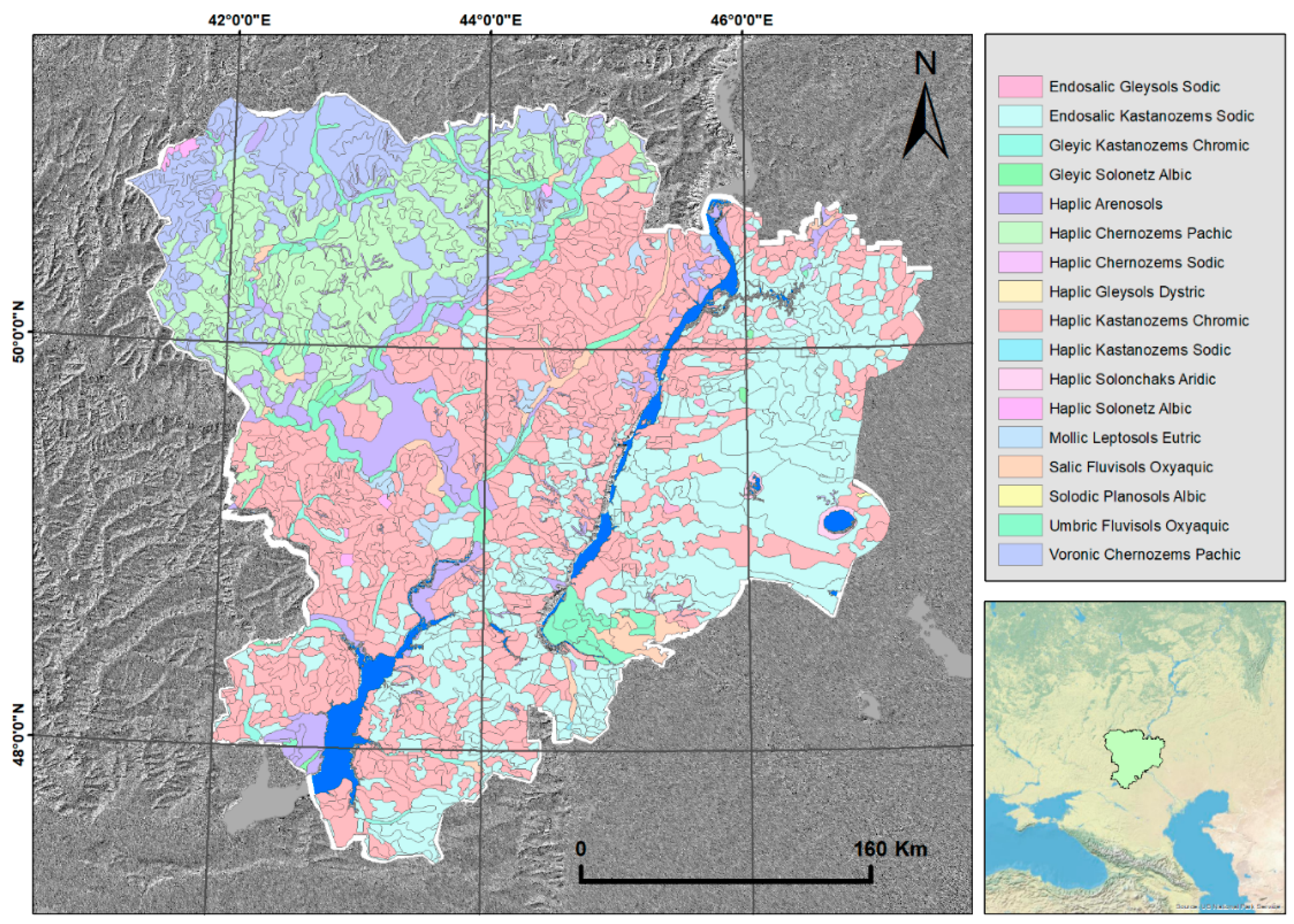
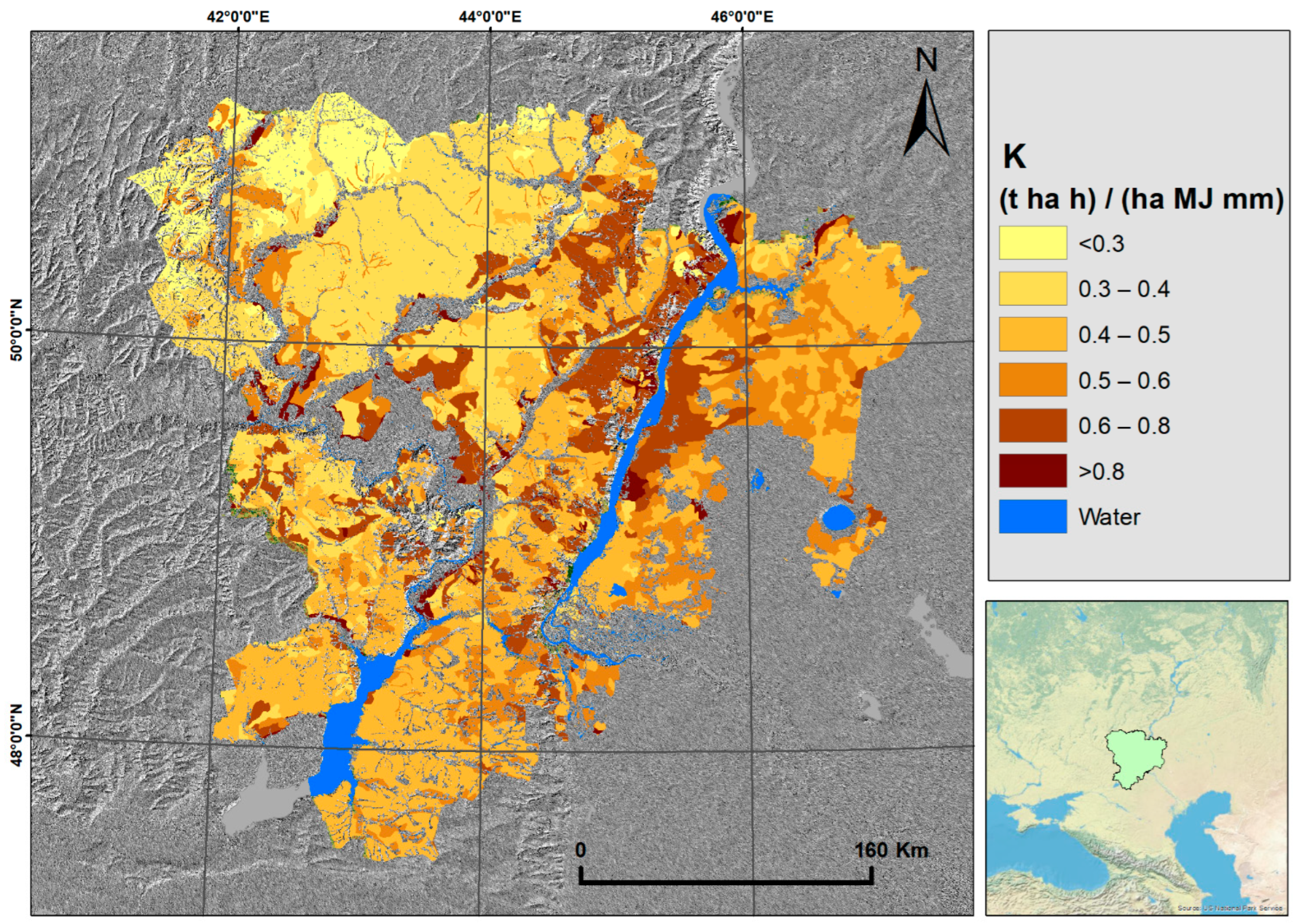
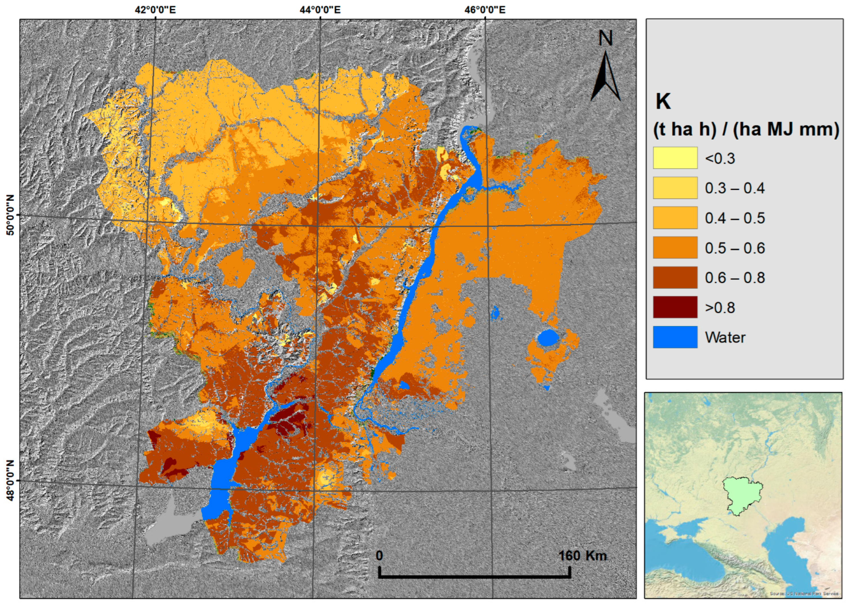
Looking at the data, we can see that the range of K-factor values increased from 0.156 to 0.973 in the 1980s to 0.182 to 0.994 in the 2010s, indicating a wider variety of soil erodibility in the latter period. The minimum K-factor value also increased from 0.156 to 0.182, suggesting that even the least erodible soils have become slightly more susceptible to erosion. The maximum K-factor value increased significantly from 0.973 to 0.994, indicating that the most erodible soils have become even more susceptible to erosion. This trend is also reflected in the average K-factor value; the average value of the K-factor increased by 19%, and the erosion resistance of the soil decreased.
The K-factor’s standard deviation (SD) decreased slightly from 0.129 to 0.088, suggesting that the variability of soil erodibility was reduced in the 2010s compared to the 1980s. The RMSE and CRPS, which are measures of the accuracy of a model’s predictions, were only available for the 2010s data, with values of 0.098 and 0.050, respectively. These values indicate that the model used to estimate the K-factor in the 2010s is reasonably accurate in predicting soil erodibility. RMSE and average CRPS for the data of the 1980s were not determined because they were calculated using a direct method based on soil map data.
According to the government data, 52% of agricultural land’s territory is subject to soil organic matter losses [58]. This is also due to the deterioration of the soil’s basic physical and chemical properties, which affect high erosion resistance, for example a decrease in organic matter content and a change in the soil texture to a lighter one. It is logical to assume that the main factor in reducing erosion resistance is the loss of soil organic matter.
The reasons for soil organic matter losses can be varied. Climate change can change the ratio of humification and mineralization processes in soil erosion. Climate change leads to changes in the ratio erosion level. On the one hand, rainfall erosivity is decreasing. On the other hand, the level of wind erosion should have been increasing. As is known, chernozems soils lost 11–25 t/ha over the last decades in the Volgograd region, or 0.3–0.8% organic matter loss through soil erosion [59]. Currently, there are no studies to assess the magnitude of wind erosion in the research area, so it is difficult to determine the wind and soil erosion by the water ratio in this area.
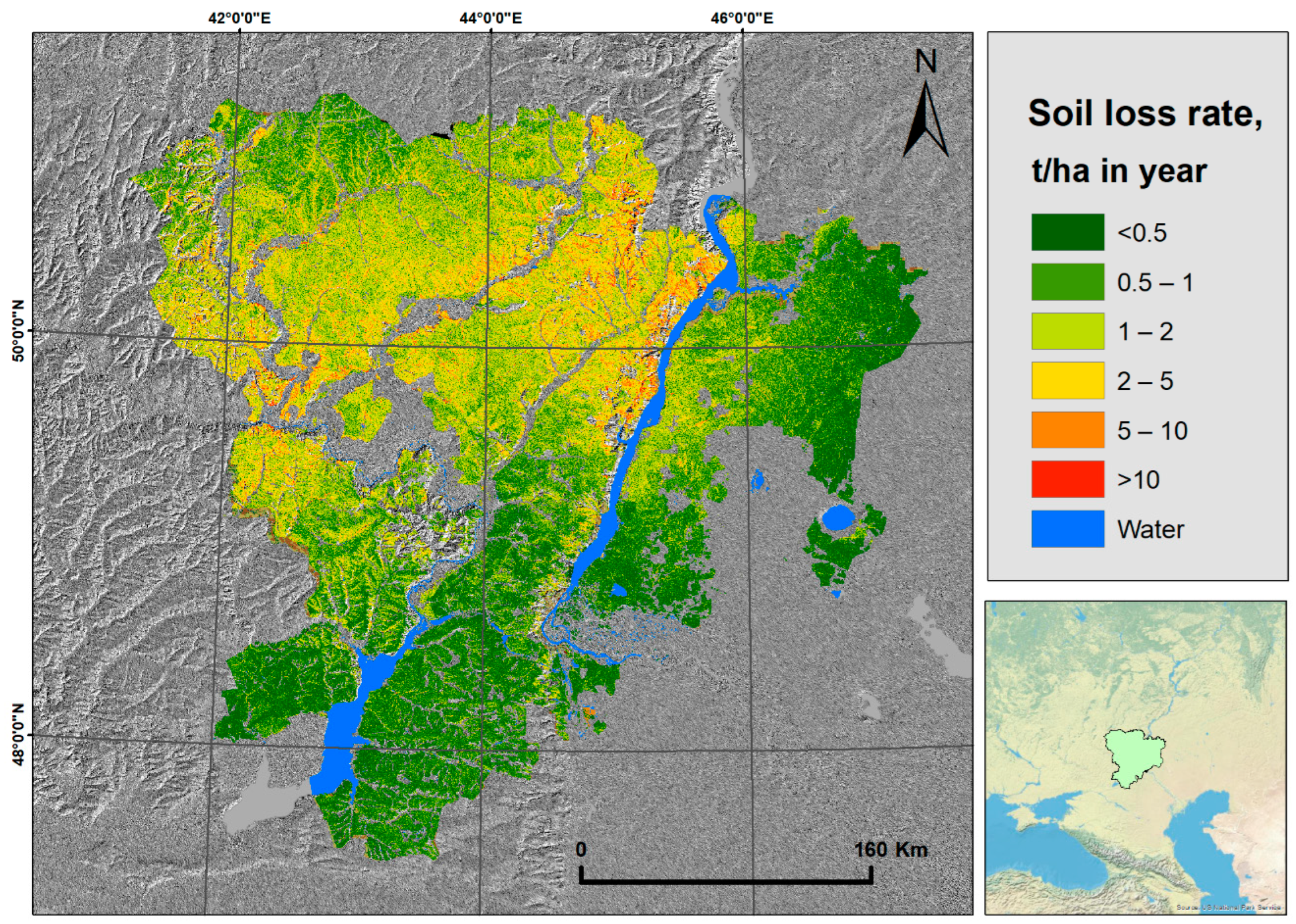
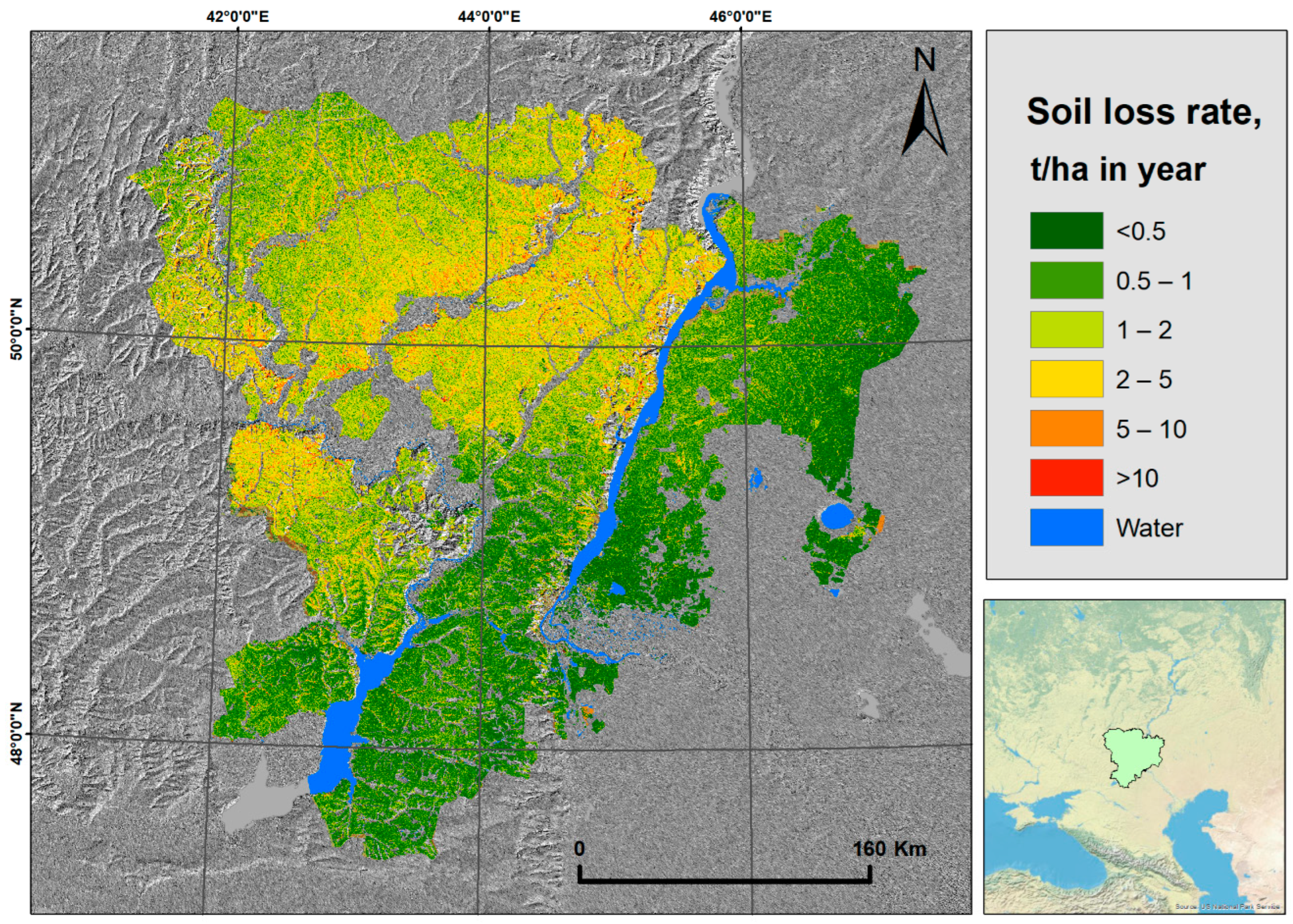
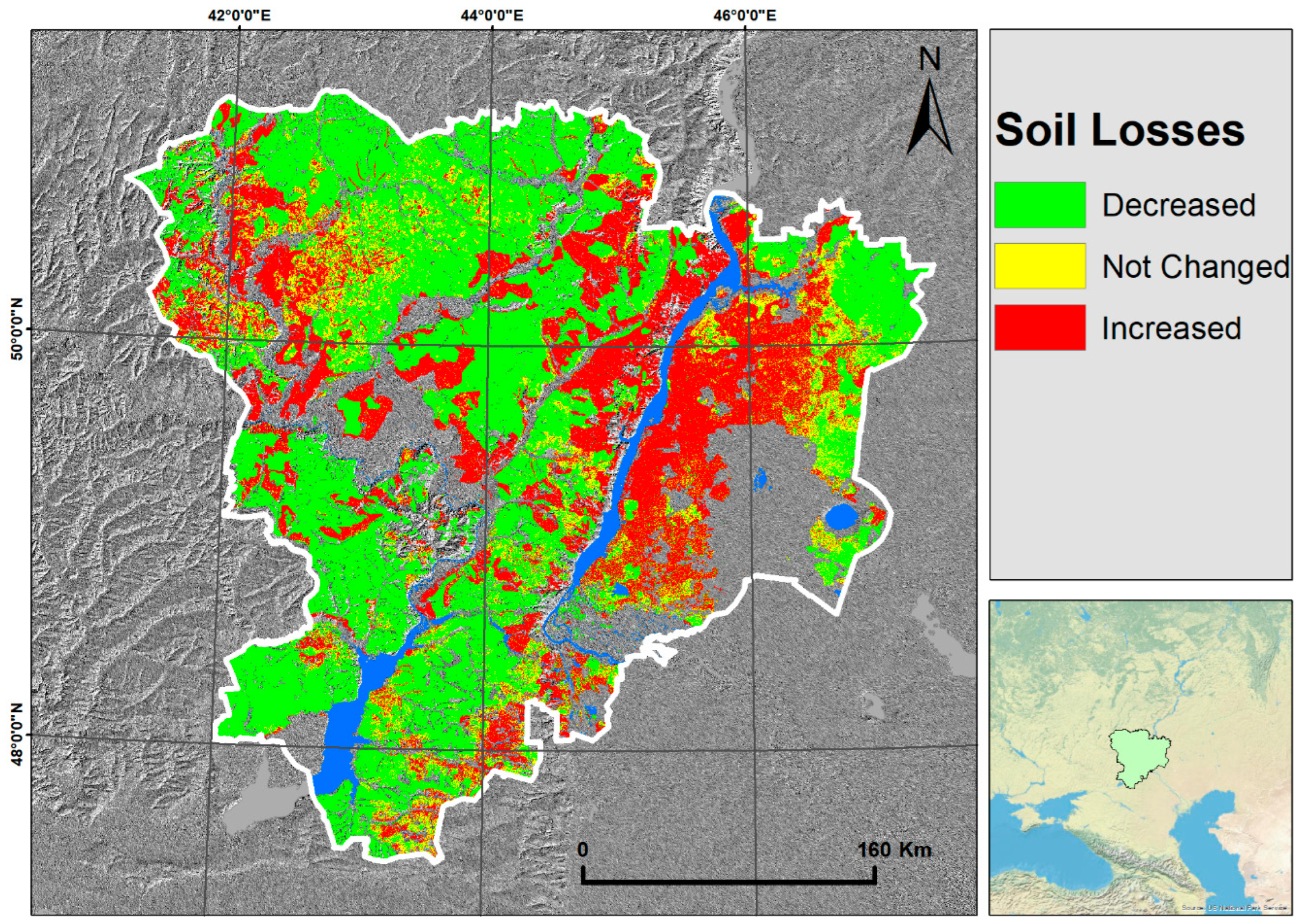
The number of soil losses in the territory of the Volgograd region had increased by 16.2% compared to 1980. That demonstrates the trend of an increase in the erosion load on the region’s territory. It is especially noticeable through the change in the structure of the distribution of the amount of soil loss: the area of contours with minimal values of soil erosion by water level (up to 1 t/ha/year) decreased, and the areas of all other shapes increased. The fact that the increase in the amount of soil erosion by water occurred against the background of two compensating phenomena—a decrease in the erosion potential of snowmelt and rainfall runoff and an increase in the protective potential of vegetation, because of changes in land use—is exciting. These processes should lead to a decrease in the territory’s soil erosion by water level. The main factor that led to this is the deterioration of the anti-erosion ability of the soil as a result of losses of SOM. About 53% of the Volgograd region’s agricultural lands are subject to SOM losses [58]. Such a wide spread of this process has led to an increase in the value of the K-factor by 19% and, as a result, an increase in the amount of soil loss.
Soil erosion by water in the region’s territory decreased from west to east and north to south. That is due to a decrease in the values of the leading actors of erosion processes—the R-factor and LS-factor. In the very northwest of the region, soil erosion by water level is also decreasing. This is due to the widespread chernozem soils, which have high erosion resistance.

4. Conclusions

This study provides quantitative and spatial data on soil erosion intensity across time in agricultural lands on a regional scale for the first time. Previous studies in this field have been restricted to specific regions in Russia or conducted on a small scale, resulting in high spatial generalization. Our research is the first attempt at the high-resolution evaluation of soil erosion by water across time. On the one hand, we suggest a new algorithm for assessing soil erosion by water levels, with good reliable results. On the other hand, certain limitations related to the quality and level of detail of the original data and unresolved methodological objectives are apparent:
(1)
The problem with soil data. The problem with open-source soil data is familiar in Russia and has been discussed many times in scientific papers [6,20]. For K-factor calculations in 2010s, we used open-source data already published in books and our own data. However, more is needed to cover the entire region. For the K-factor in the 1980s, we used a soil types map of the Volgograd region, which had a scale of 1:400 000 [37]. The simplification of the soil property’s spatial distribution, and consequently soil erosion, was significantly facilitated by this model.
(2)
The problem with the USSR’s actual areas of agricultural land. We used a present land use model for both time ranges. However, the extent of farmlands in the USSR was different from the extent nowadays. Furthermore, we need to find out how current areas match with the 1980s extent.
In order to advance research on soil erosion, obtaining more accurate assessments is crucial. To clarify the direction of future investigations, we propose the following areas of study.
(1)
Updating the rainfall erosivity (R-factor) equation for research area. In our study, we used a regression equation of the magnitude of the R-factor from the type of climate, obtained mainly for the territory of the United States, and tested in other territories. It is logical to assume that despite similar natural areas, it can work poorly in other territories. We need to collect data from all pluviographs on the territory of Russia and calculate similar equations for that area.
(2)
Calculation K-factor for 1980s based on USSR data. In our study, we assessed the K-factor based on average properties for each soil type based on the soil map of the Volgograd region. This method is ineffective because a spatial variation in the soil parameters needs to be considered. It can improve our results significantly. To do this, we must collect data from all agricultural land surveys conducted from 1980 to 1991. These data exist, but it will take time to collect, digitalize, and prepare the dataset because it is on paper sources. In our assessment, the dataset’s total points were approximately 10,000.
(3)
Define actual areas agricultural lands in the USSR time period. For defining actual USSR agricultural lands, we can use remote sensing data. The Landsat mission started in the 1970s, which can give us enough high-resolution data to define areas we need. Modern Russian land-use models have data from 2000 to the present day. Nevertheless, the areas of agricultural lands and fields were changed after the USSR collapsed. Some farms still exist, but many were closed.
(4)
Estimating wind erosion. The Volgograd region is a region where water and wind erosion exist together. The level of wind erosion increases from northwest to southeast, and soil erosion by water vice versa. Nowadays, we do not have actual data about the level of wind erosion in that region. Researchers highlight the problem of modeling soil erosion by water when wind erosion also exists in modeling. We need to set the reason for soil losses in our area precisely. For a more precise evaluation, we should also know the value of wind erosion. We also have plans for modeling wind erosion levels based on international or national models.
Within the climatic changes observed in the last four decades, including a decrease in rainfall and snowmelt runoff, and farmlands being overgrown by natural steppe vegetation, there has been a notable increase in soil losses within the Volgograd region. On average, the intensity of soil losses from the 1980s to 2010s has increased by approximately 16%, increasing from 1.48 to 1.72 t ha−1 year−1. This has happened because the soil organic matter’s massive losses are likely caused by wind erosion and soil erosion by water. Our modeling has produced similar results to other studies.
It will be possible to refine the cartographic model for predicting soil erosion in the future by incorporating more precise spatial data on soil erodibility (K-factor) and land use factor (C-factor). This will help in better understanding the reason for the decreasing soil organic matter in soils. Furthermore, wind erosion can be evaluated.

Author Contributions

Conceptualization, O.A.M.; Methodology, N.R.K.; Software, N.R.K.; Validation, N.R.K.; Investigation, N.R.K.; Writing—original draft, N.R.K.; Writing—review & editing, O.A.M.; Supervision, O.A.M.; Funding acquisition, O.A.M. All authors have read and agreed to the published version of the manuscript.

Funding

This work was supported by the Russian Fund for Basic Research (project No. 20-34-90164).

Data Availability Statement

The data presented in this study are openly available in Zenodo at 10.5281/zenodo.8385583 [60].

Acknowledgments

The authors express their gratitude to Kulik Anastasia Vladimirovna for providing archival issues of journals with data on the values of soil losses on the territory of the Volgograd region.

Conflicts of Interest

The authors declare that they have no known competing financial interests or personal relationships that could have appeared to influence the work reported in this paper.

References

  1. Wang, B.; Zheng, F.; Römkens, M.J.M.; Darboux, F. Soil Erodibility for Water Erosion: A Perspective and Chinese Experiences. Geomorphology 2013, 187, 1–10. [Google Scholar] [CrossRef]
  2. Sartori, M.; Philippidis, G.; Ferrari, E.; Borrelli, P.; Lugato, E.; Montanarella, L.; Panagos, P. A Linkage between the Biophysical and the Economic: Assessing the Global Market Impacts of Soil Erosion. Land Use Policy 2019, 86, 299–312. [Google Scholar] [CrossRef]
  3. Golosov, V.N.; Collins, A.L.; Dobrovolskaya, N.G.; Bazhenova, O.I.; Ryzhov, Y.V.; Sidorchuk, A.Y. Soil Loss on the Arable Lands of the Forest-Steppe and Steppe Zones of European Russia and Siberia during the Period of Intensive Agriculture. Geoderma 2021, 381, 114678. [Google Scholar] [CrossRef]
  4. Panagos, P.; Standardi, G.; Borrelli, P.; Lugato, E.; Montanarella, L.; Bosello, F. Cost of Agricultural Productivity Loss Due to Soil Erosion in the European Union: From Direct Cost Evaluation Approaches to the Use of Macroeconomic Models. Land Degrad. Dev. 2018, 29, 471–484. [Google Scholar] [CrossRef]
  5. Borrelli, P.; Diodato, N.; Panagos, P. Rainfall Erosivity in Italy: A National Scale Spatio-Temporal Assessment. Int. J. Digit. Earth 2016, 9, 835–850. [Google Scholar] [CrossRef]
  6. Krasilnikov, P.; Makarov, O.; Alyabina, I.; Nachtergaele, F. Assessing Soil Degradation in Northern Eurasia. Geoderma Reg. 2016, 7, 1–10. [Google Scholar] [CrossRef]
  7. Lal, R. Restoring Soil Quality to Mitigate Soil Degradation. Sustainability 2015, 7, 5875–5895. [Google Scholar] [CrossRef]
  8. Labrière, N.; Locatelli, B.; Laumonier, Y.; Freycon, V.; Bernoux, M. Soil Erosion in the Humid Tropics: A Systematic Quantitative Review. Agric. Ecosyst. Environ. 2015, 203, 127–139. [Google Scholar] [CrossRef]
  9. Tsymbarovich, P.; Kust, G.; Kumani, M.; Golosov, V.; Andreeva, O. Soil Erosion: An Important Indicator for the Assessment of Land Degradation Neutrality in Russia. Int. Soil Water Conserv. Res. 2020, 8, 418–429. [Google Scholar] [CrossRef]
  10. Colman, C.B.; Oliveira, P.T.S.; Almagro, A.; Soares-Filho, B.S.; Rodrigues, D.B.B. Effects of Climate and Land-Cover Changes on Soil Erosion in Brazilian Pantanal. Sustainability 2019, 11, 7053. [Google Scholar] [CrossRef]
  11. Graves, A.R.; Morris, J.; Deeks, L.K.; Rickson, R.J.; Kibblewhite, M.G.; Harris, J.A.; Farewell, T.S.; Truckle, I. The Total Costs of Soil Degradation in England and Wales. Ecol. Econ. 2015, 119, 399–413. [Google Scholar] [CrossRef]
  12. Safriel, U. Land Degradation Neutrality (LDN) in Drylands and beyond—Where Has It Come from and Where Does It Go. Silva Fenn. 2017, 51, 1650. [Google Scholar] [CrossRef]
  13. Grainger, A. Is Land Degradation Neutrality Feasible in Dry Areas? J. Arid. Environ. 2015, 112, 14–24. [Google Scholar] [CrossRef]
  14. Panagos, P.; Ballabio, C.; Borrelli, P.; Meusburger, K.; Klik, A.; Rousseva, S.; Tadić, M.P.; Michaelides, S.; Hrabalíková, M.; Olsen, P.; et al. Rainfall Erosivity in Europe. Sci. Total Environ. 2015, 511, 801–814. [Google Scholar] [CrossRef] [PubMed]
  15. Borrelli, P.; Alewell, C.; Alvarez, P.; Anache, J.A.A.; Baartman, J.; Ballabio, C.; Bezak, N.; Biddoccu, M.; Cerdà, A.; Chalise, D.; et al. Soil Erosion Modelling: A Global Review and Statistical Analysis. Sci. Total Environ. 2021, 780, 146494. [Google Scholar] [CrossRef] [PubMed]
  16. UNEP Climate Change 2023: Synthesis Report|UNEP—UN Environment Programme; UNEP: Nairobi, Kenya, 2023; ISBN 9789291691647.
  17. Talchabhadel, R.; Nakagawa, H.; Kawaike, K.; Prajapati, R. Evaluating the Rainfall Erosivity (R-Factor) from Daily Rainfall Data: An Application for Assessing Climate Change Impact on Soil Loss in Westrapti River Basin, Nepal. Model. Earth Syst. Environ. 2020, 6, 1741–1762. [Google Scholar] [CrossRef]
  18. Panagos, P.; Borrelli, P.; Meusburger, K.; Yu, B.; Klik, A.; Lim, K.J.; Yang, J.E.; Ni, J.; Miao, C.; Chattopadhyay, N.; et al. Global Rainfall Erosivity Assessment Based on High-Temporal Resolution Rainfall Records. Sci. Rep. 2017, 7, 4175. [Google Scholar] [CrossRef] [PubMed]
  19. Golosov, V.; Yermolaev, O.; Litvin, L.; Chizhikova, N.; Kiryukhina, Z.; Safina, G. Influence of Climate and Land Use Changes on Recent Trends of Soil Erosion Rates within the Russian Plain. Land Degrad. Dev. 2018, 29, 2658–2667. [Google Scholar] [CrossRef]
  20. Maltsev, K.; Yermolaev, O. Assessment of Soil Loss by Water Erosion in Small River Basins in Russia. Catena 2020, 195, 104726. [Google Scholar] [CrossRef]
  21. Panagos, P.; Borrelli, P.; Poesen, J.; Ballabio, C.; Lugato, E.; Meusburger, K.; Montanarella, L.; Alewell, C. The New Assessment of Soil Loss by Water Erosion in Europe. Environ. Sci. Policy 2015, 54, 438–447. [Google Scholar] [CrossRef]
  22. Plambeck, N.O. Reassessment of the Potential Risk of Soil Erosion by Water on Agricultural Land in Germany: Setting the Stage for Site-Appropriate Decision-Making in Soil and Water Resources Management. Ecol. Indic. 2020, 118, 106732. [Google Scholar] [CrossRef]
  23. Litvin, L.F.; Kiryukhina, Z.P.; Krasnov, S.F.; Dobrovol’skaya, N.G. Dynamics of Agricultural Soil Erosion in European Russia. Eurasian Soil Sci. 2017, 50, 1344–1353. [Google Scholar] [CrossRef]
  24. Litvin, L.F.; Kiryukhina, Z.P.; Krasnov, S.F.; Dobrovol’skaya, N.G.; Gorobets, A. V Dynamics of Agricultural Soil Erosion in Siberia and Far East. Eurasian Soil Sci. 2021, 54, 150–160. [Google Scholar] [CrossRef]
  25. Kulik, K.N.; Kretinin, V.M.; Rulev, A.S.; Shishkunov, V.M. The Red Book of the Soils of the Volgograd Region; Committee of Natural Resources, Forestry and Ecology of the Volgograd Region: Volgograd, Russia, 2017. [Google Scholar]
  26. Chen, J.; Chen, J.; Liao, A.; Cao, X.; Chen, L.; Chen, X.; He, C.; Han, G.; Peng, S.; Lu, M.; et al. Global Land Cover Mapping at 30 m Resolution: A POK-Based Operational Approach. ISPRS J. Photogramm. Remote Sens. 2015, 103, 7–27. [Google Scholar] [CrossRef]
  27. Renard, K.G. Science Documentation Revised Universal Soil Loss Equation Version 2. US Dep. Agric. Agric. Res. Serv. 2013, 2, 1–355. [Google Scholar]
  28. Auerswald, K.; Fiener, P.; Martin, W.; Elhaus, D. Use and Misuse of the K Factor Equation in Soil Erosion Modeling: An Alternative Equation for Determining USLE Nomograph Soil Erodibility Values. Catena 2014, 118, 220–225. [Google Scholar] [CrossRef]
  29. RIHMI-WDC RIHMI-WDC. Available online: http://meteo.ru/ (accessed on 10 October 2021).
  30. Naipal, V.; Reick, C.; Pongratz, J.; Van Oost, K. Improving the Global Applicability of the RUSLE Model—Adjustment of the Topographical and Rainfall Erosivity Factors. Geosci. Model Dev. 2015, 8, 2893–2913. [Google Scholar] [CrossRef]
  31. Peel, M.C.; Finlayson, B.L.; McMahon, T.A. Updated World Map of the Köppen-Geiger Climate Classification. Hydrol. Earth Syst. Sci. 2007, 11, 1633–1644. [Google Scholar] [CrossRef]
  32. Demidov, V.V.; Makarov, O.A. The Physical Basis of Soil Erosion: Mechanism, Patterns of Expression and Prediction: Manual; MAKS Press: Moscow, Russia, 2021; ISBN 9785317066307. [Google Scholar]
  33. Foster, G.R.; Yoder, D.G.; Weesies, G.A.; McCool, D.K.; McGregor, K.C.; Bingner, R.L. User’s Guide: Revised Universal Soil Loss Equation Version 2 (RUSLE2). US Dep. Agric. Agric. Res. Serv. 2008, 2, 1–429. [Google Scholar]
  34. Panagos, P.; Meusburger, K.; Ballabio, C.; Borrelli, P.; Alewell, C. Soil Erodibility in Europe: A High-Resolution Dataset Based on LUCAS. Sci. Total Environ. 2014, 479–480, 189–200. [Google Scholar] [CrossRef]
  35. Ministry of Agriculture. Dokuchaev Soil Institute Unified State Register of Soil Resourses of Russia. Available online: http://egrpr.esoil.ru/ (accessed on 10 October 2021).
  36. Kriuchkov, N.R.; Makarov, O.A. The Assessment of Soil and Land Degradation in Volgograd Region, the Case of Agricultural Farm Donskoe. IOP Conf. Ser. Earth Environ. Sci. 2021, 862, 012100. [Google Scholar] [CrossRef]
  37. Tsvylev, E.M. (Ed.) Soil Map of the Volgograd Region (Scale 1:400000); The Main Directorate of Geodesy and Cartography of the USSR: Moscow, Russia, 1989. [Google Scholar]
  38. Degtyareva, E.T.; Zhulidova, A.N. Soils of Volgograd Region; Nizhne-Volzhsky Book Publishing House: Volgograd, Russia, 1970. [Google Scholar]
  39. Kriuchkov, N.R.; Makarov, O.A. Slope Length and Steepness Factor (LS-Factor) for Volgograd Region (Russia) in Modeling Soil Erosion by Water. USE Prot. Nat. Resour. Russ. 2022, 3, 107–113. [Google Scholar]
  40. USGS Shuttle Radar Topography Mission (SRTM). Available online: https://dwtkns.com/srtm30m/ (accessed on 10 October 2021).
  41. Wang, L.; Liu, H. An Efficient Method for Identifying and Filling Surface Depressions in Digital Elevation Models for Hydrologic Analysis and Modelling. Int. J. Geogr. Inf. Sci. 2006, 20, 193–213. [Google Scholar] [CrossRef]
  42. Conrad, O.; Bechtel, B.; Bock, M.; Dietrich, H.; Fischer, E.; Gerlitz, L.; Wehberg, J.; Wichmann, V.; Böhner, J. System for Automated Geoscientific Analyses (SAGA) v. 2.1.4. Available online: http://www.saga-gis.org (accessed on 10 October 2021).
  43. Desmet, P.J.J.; Govers, G. Comment on ‘Modelling Topographic Potential for Erosion and Deposition Using GIS’. Int. J. Geogr. Inf. Sci. 1997, 11, 603–610. [Google Scholar] [CrossRef]
  44. Almagro, A.; Thomé, T.C.; Colman, C.B.; Pereira, R.B.; Marcato Junior, J.; Rodrigues, D.B.B.; Oliveira, P.T.S. Improving Cover and Management Factor (C-Factor) Estimation Using Remote Sensing Approaches for Tropical Regions. Int. Soil Water Conserv. Res. 2019, 7, 325–334. [Google Scholar] [CrossRef]
  45. Gribov, A.; Krivoruchko, K. Empirical Bayesian Kriging Implementation and Usage. Sci. Total Environ. 2020, 722, 137290. [Google Scholar] [CrossRef] [PubMed]
  46. Krivoruchko, K. Empirical Bayesian Kriging Implemented in ArcGIS Geostatistical Analyst; ArcUser Fall 2012; ESRI: Redlands, CA, USA, 2012. [Google Scholar]
  47. Zhang, Z.; Du, Q. A Bayesian Kriging Regression Method to Estimate Airm Temperature Using Remote Sensing Data. Remote Sens. 2019, 11, 767. [Google Scholar] [CrossRef]
  48. Zamo, M.; Naveau, P. Estimation of the Continuous Ranked Probability Score with Limited Information and Applications to Ensemble Weather Forecasts. Math. Geosci. 2018, 50, 209–234. [Google Scholar] [CrossRef]
  49. Gneiting, T.; Raftery, A.E. Strictly Proper Scoring Rules, Prediction, and Estimation. J. Am. Stat. Assoc. 2007, 102, 359–378. [Google Scholar] [CrossRef]
  50. Larionov, G.A. Soil Erosion and Deflation: Basic Patterns and Quantitative Estimates; MSU Publishing House: Moscow, Russia, 1993. [Google Scholar]
  51. Pynzar, N.M. To Substantiate the Parameters of Anti-Erosion Forest Strips in the Area of the Right Bank of the Lower Volga. Bull. All-Union Sci. Res. Inst. Agrofor. 1980, 34, 17–19. [Google Scholar]
  52. Babayan, L.A. Features agroecological status light-brown soils on the slopes south Volga region. Bull. Agroindustrial Complex Stavropol 2014, 3, 141–147. [Google Scholar]
  53. Zolotokrylin, A.N.; Titkova, T.B.; Cherenkova, E.A. Characteristics of Spring–Summer Drought in Dry and Wet Periods in the South of European Russia. Arid. Ecosyst. 2020, 10, 322–328. [Google Scholar] [CrossRef]
  54. Eltsov, M.V.; Ovchinnikov, A.Y.; Mitenko, G.V.; Alekseev, A.O. Response of Soils to Climate Change in the Steppe Zone of European Russia over the Past Decades. Eurasian Soil Sci. 2021, 54, 1808–1817. [Google Scholar] [CrossRef]
  55. Panagos, P.; Borrelli, P.; Meusburger, K. A New European Slope Length and Steepness Factor (LS-Factor) for Modeling Soil Erosion by Water. Geoscience 2015, 5, 117–126. [Google Scholar] [CrossRef]
  56. Gorokhova, I.N.; Pankova, E.I.; Kharlanov, V.A. Changes in the Ameliorative Status of Irrigated Soils of Volgograd Oblast in the 21st Century. Eurasian Soil Sci. 2019, 52, 550–565. [Google Scholar] [CrossRef]
  57. Pankova, E.I.; Novikova, A.F. Reclamation Status and Secondary Salinization of Soils of Irrigated Lands of the Volgograd Region. Eurasian Soil Sci. 2004, 731–744. [Google Scholar]
  58. Federal State Budgetary Institution Central Agrochemical Service ‘Volgogradsky’. Available online: https://агрохим34.рф/index.html (accessed on 10 October 2021).
  59. Kulik, K.N.; Barabanov, A.T.; Manaenkov, A.S.; Kulik, A.K. Forecast Assumption and Analysis of the Development of Protective Afforestation in the Volgograd Region. Stud. Russ. Econ. Dev. 2017, 28, 641–647. [Google Scholar] [CrossRef]
  60. Kriuchkov, N.; Makarov, O. Soil erosion by water in the 1980s-2020s in the steppe region of the southeast of the East European Plain (Volgograd region, Russia) [Data set]. Zenodo 2023. [Google Scholar] [CrossRef]
Figure 1. DEM.
Figure 1. DEM.
Agronomy 13 02527 g001
Figure 2. Slope.
Figure 2. Slope.
Agronomy 13 02527 g002
Figure 3. Land-use map.
Agronomy 13 02527 g003
Figure 4. Soil map.
Figure 4. Soil map.
Agronomy 13 02527 g004
Figure 5. Soil texture map.
Agronomy 13 02527 g005
Figure 6. The design of the experiment.
Agronomy 13 02527 g006
Figure 7. R-factor spatial distribution in the 1980s.
Agronomy 13 02527 g007
Figure 8. R-factor spatial distribution in the 2010s.
Agronomy 13 02527 g008
Figure 9. LS-factor spatial distribution.
Agronomy 13 02527 g009
Figure 10. C-factor spatial distribution in the 1980s.
Agronomy 13 02527 g010
Figure 11. C-factor spatial distribution in the 2010s.
Agronomy 13 02527 g011
Figure 12. K-factor spatial distribution in the 1980s.
Agronomy 13 02527 g012
Figure 13. K-factor spatial distribution in the 2010s.
Agronomy 13 02527 g013
Figure 14. Soil loss by soil erosion by water: spatial distribution in the 1980s.
Agronomy 13 02527 g014
Figure 15. Soil loss by soil erosion by water: spatial distribution in the 2010s.
Agronomy 13 02527 g015
Figure 16. The difference in soil loss between the 1980s and 2010s.
Agronomy 13 02527 g016
Table 1. Definition of soil structure index.
Soil Structure IndexDescription
1Very fine granular: 1–2 mm
2Fine granular: 2–5 mm
3Medium or coarse granular: 5–10 mm
4Blocky, platy, or massive: >10 mm
Table 2. Definition of soil permeability index.
Soil Permeability IndexDescription
1Sand
2Loamy sand, sandy loam
3Loam, silty loam
4Sandy clay loam, clay loam
5Silty clay loam, sand clay
6Silty clay, clay
Table 3. Statistical characteristics of the R-factor in (Mj mm)/(ha h g).
YearMinimumMaximumAverageSDRMSECRPS
1980s37.15247.06135.8564.7018.158.44
2010s24.89216.08123.7574.7125.7513.31
Table 4. Percentage distribution by classes of R-factor values in %.
YearClasses
<6060–100100–140140–190>190
198012.1328.209.6620.2929.72
201024.7018.569.6630.1116.97
Changes+12.57−9.640.00+9.82−12.75
Table 5. Statistical characteristics of the LS-factor.
LSMinimumMaximumAverageSD
0.035035.510.522.20
Table 6. Percentage distribution by classes of LS-factor values.
LSClasses
<0.10.1–0.50.5–11–2>2
2.6866.1923.285.921.93
Table 7. Statistical characteristics of the C-factor.
YearMinimumMaximumAverageSD
1980s0.0260.0550.0420.003
2010s0.0240.0570.0400.003
Table 8. Percentage distribution by classes of C-factor values.
YearClasses
<0.0360.036–0.0380.038–0.0400.040–0.0420.042–0.046>0.046
1980s2.344.4310.5620.2558.394.03
2010s7.709.0518.4632.2732.350.17
Changes+5.36+4.62+7.90+12.03−26.04−3.87
Table 9. Statistical characteristics of the K-factor.
YearMinimumMaximumAverageSDRMSECRPS
1980s0.1560.9730.4750.129--
2010s0.1820.9940.5660.0880.0980.050
Table 10. Percentage distribution by classes of K-factor values.
YearClasses
<0.30.3–0.40.4–0.50.5–0.60.60–0.80>0.8
1980s6.5628.1033.6016.2513.362.14
2010s0.281.5220.6850.3225.921.28
Changes−6.28−26.57−12.9334.0712.56−0.86
Table 11. Statistical characteristics of soil losses by soil erosion by water.
YearMinimumMaximumAverageSD
1980s0.01643.241.481.91
2010s0.23465.121.726.06
Table 12. Percentage distribution by classes of soil losses by soil erosion by water.
YearClasses
<0.50.5–11–22–55–10>10
198022.8029.2027.8716.472.870.78
201020.9628.4728.9717.462.951.19
Changes−1.84−0.731.090.990.080.41
Table 13. Comparison of the results obtained with other studies.
SourceAnnual Soil Loss, 103 t,
1980s
The Difference in the Results Obtained, %Change in Mean
Annual Soil
Erosion
Rate *, % (±)
The Difference in the Results Obtained, %
Kriuchkov, Makarov, 20238636.10-+16.2-
Litvin et al., 2017 [23]9919.80+12%+23.4+7.2%
Golosov et al., 2018 [19]--+18.7%−2.5%
* From the 1980s to 2010s.
Table 14. Comparison of the results with the results of field studies.
SourceSoil Loss, t ha−1 year−1Soil Loss, t ha−1 year−1 (Kriuchkov, Makarov 2023)The Difference in the Results Obtained, %
Babayan, 2014 [52]12.310.515%
Pynzar, 1980 [51]0.510.486.3%
Disclaimer/Publisher’s Note: The statements, opinions and data contained in all publications are solely those of the individual author(s) and contributor(s) and not of MDPI and/or the editor(s). MDPI and/or the editor(s) disclaim responsibility for any injury to people or property resulting from any ideas, methods, instructions or products referred to in the content.

