Abstract
Increasing crop yield is a significant objective in modern agriculture, with adjusted planting density and rational fertilization strategies standing out as the foremost approaches for attaining such a goal. Through the use of modern artificial intelligence techniques such as genetic algorithms and neural networks, the CPDOS (Crop Planting Density Optimization System), an online intelligent system that can automate the modeling, optimization, and analysis of the two models, was developed in the present study. The goal of the system is to optimize the planting density model and fertilizer application in combination with other computer system development techniques. The CPDOS comprises three main modules: yield density optimization module, optimal planting density range module, and fertilization and planting density optimization module. The three modules are complemented by two modules for data input and result visualization, culminating in the comprehensive process of optimizing planting density and fertilizer allocation through the CPDOS. The CPDOS was tested using potato, corn, and soybean data, and the results show that the optimization effects of planting density and fertilizer application were satisfactory. The CPDOS is an automated crop planting optimization system that integrates algorithms and models and is driven by artificial intelligence technology. The introduction of the CPDOS reduces the barriers to utilizing these algorithms and models, facilitating wider adoption of intelligently optimized planting technology. The platform’s launch will accelerate the swift advancement of this field.
1. Introduction
Food is a fundamental necessity for human survival and progress, having a considerable influence on economic dynamics, individual well-being, and the social stability of countries and regions [1]. Arable land in China occupies less than 10% of the world’s landmass [2], while China accounts for over 20% of the world’s population. Given this context, food-related challenges are intricately tied to China’s economic progress and social stability.
Crop planting density serves as the foundation for crop population change, which is closely related to crop population size, light energy utilization, and yield, standing out as a pivotal determinant in agricultural production [3]. As such, research on the effect of different crop planting densities on crop yield has emerged as a common topic in grain yield studies. Since the 1950s, numerous agricultural researchers have attempted to quantitatively define the relationship between planting density and crop yield. To that end, a series of widely recognized yield–density models have been adopted [4]. Holliday proposed that the relationship between planting density and crop yield can be divided into two types of relationships. The first is a progressive relationship, wherein as density increases, the yield attains its peak and remains constant at elevated densities. The second type entails a parabolic relationship, whereby the yield rises with augmented density until it reaches its maximum value, subsequently tapering off gradually at higher densities. Holliday’s research laid the foundation for subsequent research on the relationship between yield and density [5]. Shinozaki et al. derived an equation to describe the progressive yield–density relationship based on the logistic growth curve combined with the final yield stability law. This equation is akin to the one derived by Holliday in 1960 and is often employed to depict the asymptotic relationship between yield and density [6].
At the same time, planting density and fertilizer application are other significant factors that affect crop yield and quality. Consequently, the optimization of planting density and fertilizer application aligns more effectively with the needs of actual agricultural production. Through a block design, Fanga et al. found that the volume of nitrogen fertilizer and planting density had significant effects on the photosynthetic capacity, characteristics, and yield of buckwheat leaves [7]. Zhou et al. discovered that the key attributes of rice grain quality, encompassing their milling properties, visual appearance, nutritional composition, and cooking characteristics, were influenced by the specific rice variety. Notably, significant variations existed between distinct rice varieties in terms of these attributes. Nitrogen fertilizer application and increased planting density can improve grain quality [8]. Tang et al. evaluated the effects of planting density and nitrogen application rate on cannabis stem and seed yield under eight different environments at five comparative locations in Europe. Their findings were that planting density had limited effects on yield, while plant height and stem diameter decreased with increasing population density [9].
The agricultural sector is harnessing information and communication technology to enhance productivity and minimize losses. However, given that many agricultural producers lack familiarity with cutting-edge technologies and methodologies, the development of expert systems becomes essential to offer guidance and support [10]. González-Esquiva et al. developed a Web application system that supports the remote monitoring of crops, including the ability to upload, analyze, and visualize images and store data. By using the histogram-based probabilistic color model and Fuzzyc-means algorithm to cluster in the RGB (RedGreenBlue) space, two color segmentation techniques were employed to estimate the green coverage from digital images and evaluate the crop irrigation requirements [11]. The main focus of existing research has been on the relationship between planting density and crop yield, and a series of widely accepted yield–density models have been formulated. Despite such research efforts, challenges arise due to the predominantly nonlinear nature of yield–density models. Inadequate computational capabilities, elevated operational expenses, intricate model parameter estimations, and substantial errors limit the extensive adoption and utilization of such models to a certain extent.
The research purpose of the present study was to leverage modern computing technology for optimizing planting density, thereby fostering noteworthy research outcomes. Such outcomes can provide a critical reference and basis for the development of intelligent crop planting plans. Firstly, six classical yield–density models were selected, and a genetic algorithm was used to estimate and optimize the model parameters. Subsequently, the model that best aligned with the current dataset was identified and selected. Secondly, after formulating the optimal yield–density model and considering the production costs, the quantitative relationship between economic yield and planting density was obtained, and the optimal planting density range was calculated. Finally, based on the obtained outcomes, a crop planting density optimization system was developed and implemented. The system comprises three core modules: yield density optimization module, optimal planting density range module, and fertilization and planting density optimization module. Using the system, users can better analyze existing data such as yield–density, and realize planting density optimization. The CPDOS has been published in the Ali cloud server, web address: http://8.142.2.157/index_e, accessed on 1 June 2022. The supplementary document contains detailed operating steps and has uploaded a guide video for using the CPDOS, web address: https://www.bilibili.com/video/BV1Vp4y1A7sf/?share_source=copy_web&vd_source=30491301abc6fb3d84754366222bc8c9, accessed on 1 June 2022. The CPDOS platform is freely available for all academic and non-commercial users for free and can only be used for research purposes!
2. Materials and Methods
2.1. Overview of Methods
The research method is divided into two main parts: the crop planting density optimization method and the crop planting density optimization system realization method.
- (1)
- Crop planting density optimization method
The CPDOS mainly uses a genetic algorithm, dichotomy, polynomial regression, and a BP (Back Propagation) neural network. Six classical yield–density models were obtained after consulting a large number of literature studies, and a genetic algorithm was used to estimate the parameters and select the best yield–density model. Then, considering the crop production cost, the optimal planting density range when the economic yield reaches its expected range was calculated. This part uses the dichotomy to solve the equation. Finally, a BP neural network and polynomial regression were used to analyze the planting density data and fertilization amount, and a genetic algorithm was used to optimize the combination of planting density and amount of fertilizer to achieve the highest yield.
- (2)
- Implementation of CPDOS
The two core functions of the CPDOS are model parameter estimation and model selection based on a genetic algorithm and the optimal planting density calculation. The CPDOS adopts the B/S (Brower/Server) system structure, which is divided into three layers: system front end, system back end, and system database. The system development mostly uses Python language, the web application framework uses the Django framework, the front-end framework uses Vue, Semantic UI, and jQurey, which are based on HTML, CSS, and JavaScript, and data visualization is realized by PyeCharts. MySQL relational database management system is selected as the database.
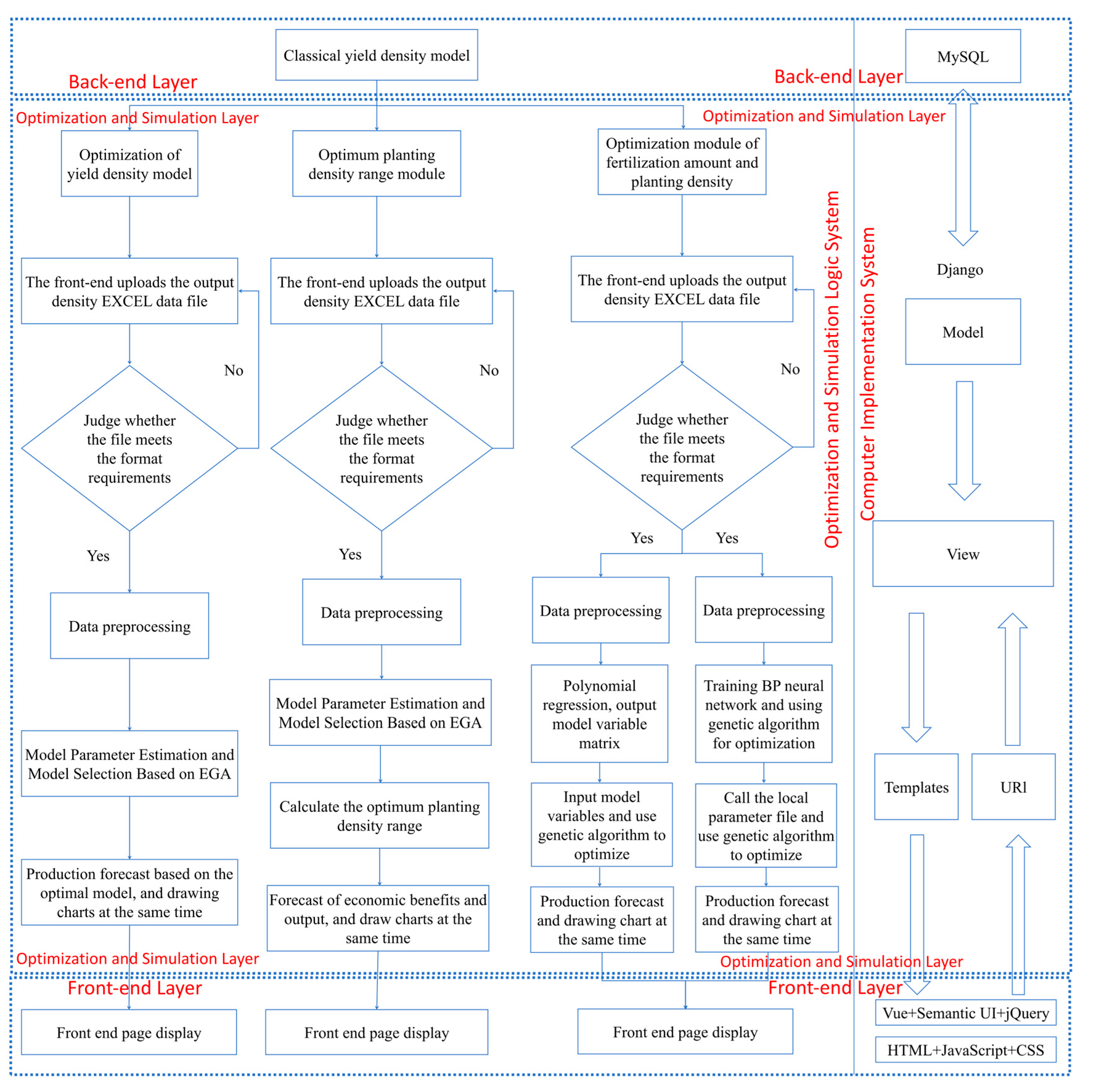
The technical roadmap of the CPDOS is shown in Figure 1.
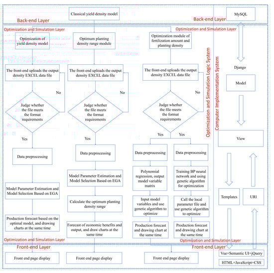
Figure 1.
Technical roadmap of crop planting density optimization system.
2.2. Experimental Data
2.2.1. Potato Yield–Density Data
The experimental data for the parameters estimation and crop yield–density model selection of potatoes in this study were extracted from Mo Huidong’s [12] potato yield–density data, as presented in Table 1. Since the data include production costs for each density (the cost of planting potatoes in the original text was GBP (Pound) 18 per ton, and the production cost was converted to the corresponding yield consumption based on the unit price of each density tuber in the original text), we also analyzed the economic benefits.

Table 1.
Potato yield–density data of Mo Huidong.
2.2.2. Maize Yield–Density Data
The optimum planting density range experimental data of the maize yield–density model in this study was selected from the maize yield–density data of Mo Huidong [12], as presented in Table 2. The production cost data in the table include various operating costs and material costs in crop production, according to a maize unit price of 0.16 CNY/kg converted into maize production consumption during the production process.
Table 2.
Maize yield–density data of Mo Huidong.
2.2.3. Soybean Yield–Density Data
In this study, the experimental data of Xuguang [13] were selected to optimize the optimal planting density and fertilization ratio when the crop yield was the largest, as shown in Table 3.
Table 3.
Liang Xuguang’s soybean data.
2.2.4. Yield–Density Data of Different Crops
In this study, the experimental optimal yield–density model data of different crops were selected. The crops included potato [14], sorghum [15], pepper [16], peanut [17], sesame [18], wheat [19], and soybean [20]. The specific data are shown in Tables S1–S7.
2.3. Technical Route
The crop planting density optimization system was designed to help agricultural production personnel and researchers to better analyze crop yield and planting density data, as well as fertilizer application and planting density data. It also aimed to assist in planting density and planting-density-to-fertilizer-application ratio decisions. Therefore, the system needed to have a user-friendly interface and be simple to operate. The system realizes the data visualization function, which can draw the model curve diagram and the correlation test diagram, which can help users intuitively understand the system operation results. In addition to the visualization module, the system also includes a user login registration module, a yield–density model optimization module, an optimal planting density range module, and a fertilization or planting density optimization module.
2.4. Running CPDOS
The CPDOS mainly implements the following functions:
- (1)
- The user can obtain the yield–density equation of different crops under different environments by inputting the yield–density data and understanding the change rule between individual yield and population yield under different densities.
- (2)
- By inputting the production cost, planting density, and yield data, the user can obtain the optimal yield–density equation matching the current data, and the best economic yield can be obtained.
- (3)
- Users input the planting density, fertilization data, and yield data. The system performs quadratic polynomial regression and BP neural network regression, respectively, and obtains the best planting density and fertilization ratio in each regression model.
- (4)
- Data visualization is realized and the yield–density curve and the model’s goodness-of-fit verification diagram are drawn to better display the calculated results.
Users need to log in and register before using the other functional CPDOS modules. When registering, if the user inputs their username, mobile phone number, and password in the format specified by the system, the system will store the user data and complete the registration. In order to facilitate the user, the system will automatically log in the user after successful registration, therefore avoiding repeated logins. During the user login process, if the user forgets their username, they can log in by entering their mobile phone number. After the username and password are verified, the user can use the other functional modules. When the user enters their username and other information, the page detects the input character format, and if it does not conform to the format specified by the system, the page will jump out of the prompt character. Only when all the inputs match the format and the username and mobile phone number are not repeated will the registration be completed. After successfully registering, the system will automatically log on, eliminating any repeated input. The CPDOS can choose the next auto-login when it logs in, and the browser will remember the user information for two weeks.
The implementation of the CPDOS yield–density model optimization module is as follows: after the user uploads the yield–density model file to the page, the back end of the system tests the uploaded file format. After the test is passed, a Panda data analysis package is used for data preprocessing; a genetic algorithm is used to estimate the parameters, based on the uploaded data, and the model is selected. The back end uses the selected optimal yield–density model for yield prediction, and the optimal model fitting results are uploaded to the front end for the page display. The yield–density model optimization module data visualization takes two forms, a chart and a model curve and goodness-of-fit chart. The initial chart display is realized by DataTables and mainly shows a combination of the yield–density data uploaded by the user and the yield data predicted by the optimal yield–density model. For user convenience, the table also realizes page-turning, querying, and sorting. The graph is mainly created through PyeCharts. Using Pyecharts in Django can be described in three main steps: data preparation, back-end drawing and uploading to the front-end, and front-end rendering.
The CPDOS optimal planting density range module can be implemented as follows: when the user uploads the data file, the system tests the file format, preprocesses the data, and then uses the above optimal planting density range calculation method to obtain the upper and lower limits of the planting density. The chart is then drawn, and the calculation results are uploaded to the front end, where page rendering is performed. The optimal planting density range display page is also laid out through the Semantic UI tab syntax. A total of three tabs are assigned; data tables, optimal planting density range, and analysis results visualization. The optimum planting density range tab shows the specific results of the optimum yield–density and economic benefit models, while the remaining two tabs are used for data visualization. The optimal planting density range module data visualization display is divided into a data table and a diagram. In addition to displaying the data uploaded by users, the data table also shows the predicted yield data using the optimal yield–density model and the economic benefit yield data predicted by the economic benefit yield model. The drawing shows a diagram of the optimum planting density range based on the graphic method and the curve of the optimum yield–density model and goodness-of-fit test.
A CPDOS based on the BP neural network planting density fertilizer ratio optimization module is implemented as follows: after data are submitted by the user, the system uses the BP neural network and polynomial regression based on the fertilizer amount and planting density optimization method to predict the yield and draw the charts via front-end rendering and display. The data visualization display can be divided into three parts. The first is the BP neural network fitting result. This displays the forward propagation equation of the BP neural network, the local file storage address of the BP neural network weight, and the network fitting result. The second shows the goodness-of-fit test of the BP neural network. The third part presents the results of the genetic algorithm optimization, the maximum yield optimization, and the corresponding planting density and fertilizer ratio.
The results page of the CPDOS optimal planting density fertilization ratio optimization module, based on polynomial regression, can also be divided into three sections. The first is the polynomial regression fitting results. This shows the polynomial regression equation, the polynomial regression equation parameter vector, and the fitting results. The second shows the polynomial regression goodness-of-fit diagram. The third part presents the genetic algorithm optimization results, the maximum yield optimization, and the corresponding planting density and fertilizer ratio.
The entire CPDOS operational process is presented in Figure 2.

Figure 2.
The whole process of CPDOS running. (A) user registration; (B) user login; (C) click start on CPDOS homepage; (D) click “Browse”; (E) “Upload” EXCEL file; (F) upload data display; (G) parameter estimation and selection of optimal yield–density model; (H) visualization of analysis results of optimal yield–density model.
2.5. Crop Yield–Density Model for CPDOS
2.5.1. Progressive Yield–Density Model
Japanese scholar K. Shinozaki et al. [6] derived the equation describing the yield–density relationship of the asymptotic shape based on the logistic growth curve combined with the final yield stability law, see Formulas (1) and (2), then Holliday and De Wit et al. derived the same equation via different methods. Formulas (1) and (2) are generally accepted equations to describe the relationship between asymptote yield and density [12].
2.5.2. Parabolic Yield–Density Model
When Fan Furen and Mo Huidong studied the relationship between maize yield and density, they found that when the planting density, , changed according to the arithmetic progression, , which changed according to the geometric progression. That is, for each unit increase in x, the number of plants to be increased for each unit of yield is a geometric constant [21]. The specific forms of the model are shown in Formulas (3) and (4). Duncan W G [22] and Carmer S G [23] have proposed the parabolic yield–density model in similar form.
2.5.3. Mixed Yield–Density Model
Farazdaghi and Harris believed that the final yield stability law was not always true, so they modified the final yield stability law and derived the following mixed yield–density model I [24] by combining the logistic growth curve:
In the model when the model is the same as the progressive yield–density model proposed by Shinozaki et al. When the model describes the parabolic yield–density relationship. Therefore, this model is a mixed model, through the change in parameters can describe the progressive yield–density relationship or parabolic yield–density relationship.
Holliday classified the yield–density relationship into progressive relationship and parabolic relationship. For the asymptotic relationship, Holliday’s model is actually Formulas (1) and (2). For the parabolic relationship, Holliday proposed the following mixed yield–density model II [5]:
In the model, and are parameters that are greater than 0. Ding Changling [25] also deduced Equation (8) through the relationship between panicle weight and panicle number of rice. The model is obviously mixed model, and when Formula (7) is the same as Formula (1). When the model describes a parabolic relationship. When discussing the basic properties of the model, only the case of is discussed.
Holliday [5] explained the biological significance of the parameters in the model in a different way. He realized the importance of parameter because the maximum yield per plant is 1/ he set and called it the apparent maximum yield, representing the potential of crops. Bring into the parabolic yield–density model, the model form becomes
Holliday called the expression a competition function, which decreases with an increase in planting density, . On this basis, Holliday gives a realistic description of yield per plant, that is, yield per plant is the product of the crop potential, and competitiveness, acting on crops.
Bleasdale and Nelder [26] believe that a model can be used to describe all cases of the yield–density relationship. Bleasdale and Nelder derived a yield–density model:
In Equation (11), and are model parameters. When the model can describe the progressive yield–density relationship; when the parabolic yield–density relationship can be described. However, Bleasdale et al. [26] found that yield–density data were rarely accurate enough to determine estimates of both and so they simplified the model by setting to obtain the following mixed yield–density model III:
In the model, are greater than 0, and the value interval of is generally . When the model is the same as Equations (1) and (2), which describes the progressive yield–density relationship. When is in the interval it describes the parabolic yield–density relationship. When discussing the basic properties of the model, only the case of in the interval is discussed.
Hudson et al. [27] first used a quadratic expression to describe the relationship between the grain yield and grain rate of winter wheat. Later, Stanger and Lauer [28], Coulter et al. [29] and Van Roekel and Coulter et al. [30] fitted yield–density data well by using quadratic expressions. Yared Assef et al. fitted the yield–density data by using a linear model, exponential model, hyperbolic model, and quadratic model and compared the fitting effect of the model by its coefficient of determination (), Akaike information criterion (AIC), modified Akaike information criterion (AICC) and Bayesian information criterion (BIC). Finally, it was found that the fitting effect of the quadratic model was generally better than other models [31]. The expression of mixed yield–density model IV is shown in Equation (14):
In the quadratic model,.
2.6. CPDOS Parameter Estimation of Yield–Density Model and Selection of Optimal Yield–Density Model Based on EGA (Evolutionary Genetic Algorithm)
The six yield–density models selected in this paper are all nonlinear models. It is the complex parameter estimation that limits the promotion of these excellent research results. Secondly, the methods of model parameter estimation are often different for different nonlinear models. At present, there is no parameter estimation method suitable for all nonlinear models. Therefore, if we can find a parameter estimation method that does not depend on the expression of the nonlinear model, it means that the method of parameter estimation for general nonlinear systems has been found. In this paper, the EGA (Evolutionary Genetic Algorithm) combined with the least-squares method is used to estimate the parameters of the selected six yield–density models, and the mean square error MSE (Mean Square Error) is used as the model selection criterion to select the best yield–density model matching the current data. The simulation results of this method are compared with other methods to verify the practicability and effectiveness of this method.
2.6.1. CPDOS Genetic Algorithm EGA Strategy Design
The classical genetic algorithm may destroy the individual with the highest population fitness when performing genetic operations such as random selection, crossover, and mutation. Therefore, this study uses the elite retention strategy to optimize the classical genetic algorithm. The individual with the highest contemporary fitness is retained as an elite individual, and the remaining individuals generate new individuals through random selection, crossover, and mutation and merge the elite individuals and new individuals to form a new population. This method improves the global convergence and robustness of the classical genetic algorithm. The CPDOS uses the EGA (Evolutionary Genetic Algorithm) for model parameter estimation and model screening. The steps mainly include coding and population initialization, setting fitness function, selection, crossover, mutation, elite retention strategy, and model screening.
- (1)
- Coding population initialization
The coding design is a key element in using evolutionary algorithms to solve practical problems. Coding is the process of mapping the solution space of the problem to the coding space (search space). The mapping from the coding space to the solution space of the problem becomes decoding. The way of encoding has a great influence on the search process. According to the data type classification of coding results, encoding can be one-dimensional or two-dimensional data columns, binary data columns, or strings. According to the mapping method of classification, coding can be simple mapping coding, multiple mapping coding, permutation coding, tree coding, etc. In general, coding needs to meet three principles:
➀ Completeness: all points in the solution space of the problem can be mapped to points in the coding space (i.e., chromosomes).
➁ Reliability: the encoded chromosome must correspond to a potential solution in the problem space.
➂ Non-redundancy (not mandatory): there must be one-to-one correspondence between chromosomes and potential solutions.
Binary coding is the most important coding method in the genetic algorithm. It represents the parameters of space as a chromosome bit string composed of character set [0, 1], and the individual genotype is a binary coding symbol string. The length of the binary coded symbol string is related to the solution accuracy required by the problem. The binary encoding and decoding operation is simple, and the crossover, mutation, and other genetic operations are needed to facilitate the realization of a strong spatial search capability. Therefore, it is more suitable for solving numerical optimization problems. The parameter estimation of crop planting density model is a numerical optimization problem, so this paper uses binary coding.
- (2)
- Population initialization
Before the genetic operation, a group of initial populations must be generated, which should be evenly distributed in the solution space of the parameters and actually represent the set of some possible solutions to the optimization problem. The size of the population determines the search ability of the genetic algorithm. The size of the population is a very important parameter. The larger the size, the higher the diversity of the population and the more likely it is to search for the global optimal solution, but the corresponding amount of calculation increases. If the population is too small, the convergence speed is accelerated but may fall into a local optimal solution. In order to strengthen the robustness of the EGA (Evolutionary Genetic Algorithm) method and avoid falling into the local optimal solution as much as possible, this paper uses a larger population size and a higher mutation probability to make the EGA (Evolutionary Genetic Algorithm) skip the local optimal solution through mutation. This article sets the population size to 200.
- (3)
- Set the fitness function
Individuals in the population are evaluated by a fitness function, and excellent individuals with high fitness are selected and inherited to the next generation. The selection of the fitness function directly affects the convergence performance and output results of the algorithm. This paper is based on the least-squares method for parameter estimation. The parameter estimation problem of the crop yield–density model can be defined as the problem of using simulated data and real data to correct the model parameters and finally minimize the error between the simulated value and the real value. Assuming that the parameters of the model are and respectively, m is the actual number of measurements, and the true and simulated values of the model output are and respectively, then the fitness function of the EGA (Evolutionary Genetic Algorithm) can be expressed as
The parameters and can be obtained by minimizing .
- (4)
- Selection strategy
The genetic algorithm uses selection operators to operate on individuals: according to the fitness value of each individual, individuals with high fitness are more likely to be inherited into the next generation group; individuals with lower fitness are less likely to be inherited into the next generation. In this way, the fitness value in the group can be constantly close to the optimal solution. Commonly used selection methods are roulette selection, random competition selection, best retention selection, tournament selection, etc. In this paper, the genetic genes were selected using the tournament selection method. This selection strategy can avoid premature convergence and stagnation to a certain extent. The specific strategy of the tournament selection method is the following: randomly select k individuals from the population (the probability that each individual is selected is the same), select the individual with the best fitness as the parent of the next generation, and repeat the operation until the new population size reaches the original population size.
- (5)
- Cross strategy
The so-called crossover operation in the genetic algorithm refers to the exchange of some genes between two mutually paired chromosomes in some way to form two new individuals. The crossover operation is an important feature of the genetic algorithm that is different from other evolutionary operations. It plays a key role in the genetic algorithm and is the main method for generating new individuals. The commonly used crossover operators are single-point crossover, double-point crossover, multi-point crossover, and uniform crossover. The research shows that for the complex multi-parameter estimation problem, the effect of double-point crossover is better than that of single-point crossover. In this study, the model parameter estimation problem is a multivariate optimization problem, so the double-point crossover strategy is adopted.
Crossover probability is a parameter used to control the crossover operation of individuals, and its value directly affects the crossover result. Generally speaking, in the early stage of the genetic algorithm, the difference between individuals is large, and it is not suitable to adopt a large crossover probability, which can easily destroy the excellent individual gene prematurely. In the later stage of the operation, the population individuals tend to be similar, and using too small a probability will make the optimization search of the genetic algorithm stagnate or converge to the local optimal solution. Considering the operation and specific problems, the general crossover probability value range is 0.4–0.9. This study used 0.7.
- (6)
- Variation operation
The mutation in the genetic algorithm is used to simulate the phenomenon of gene mutation in the process of biological evolution. Its setting is mainly chosen to prevent premature convergence and maintain the diversity of the population. In the mutation operation, the value of the mutation probability is very critical. If the value is too large, i.e., if it is greater than 5, the genetic algorithm will degenerate into a random search. This value is too small to maintain diversity. In order to prevent the model from premature convergence and falling into a local optimal solution, this paper adopts a larger population size and a larger mutation probability. This paper uses the basic bit mutation algorithm, and the mutation probability is set to 0.2.
- (7)
- Elite retention strategy
The elite retention strategy is to save the individuals with the optimal fitness value searched for in each generation of population evolution as elite individuals, and then perform genetic operations on the remaining N-1 individuals to avoid the loss and destruction of the best genes in the current population. Using the EGA (Evolutionary Genetic Algorithm) to fit the yield–density model parameters has the following advantages: (1) It retain the parallelism of the traditional GA, the algorithm efficiency is high, and model parameter extraction time is saved. (2) The introduction of the elite retention strategy improves the search speed of the traditional GA, and the global convergence is faster.
- (8)
- Model screening
Different yield–density data have different fitting effects in different yield–density models. In order to find the yield–density model that best matches the current data, this paper uses the EGA (Evolutionary Genetic Algorithm) to estimate the parameters of the selected 6 yield–density models at the same time. By using the mean square error MSE as the model screening standard, the optimal yield–density model under the current data set is selected.
2.6.2. Parameter Estimation of Yield–Density Model and Selection of Optimal Yield Density Model
Geatpy is a high-performance and practical evolutionary algorithm toolbox. It provides many library functions for important operations in the implemented evolutionary algorithms and provides a highly modular and low-coupling object-oriented evolutionary algorithm framework. It uses the pattern of ‘defining problem classes + calling algorithm templates’ to perform evolutionary optimization, which can be used to solve single-objective optimization, multi-objective optimization, complex constraint optimization, combinatorial optimization, hybrid coding evolutionary optimization, and other problems.
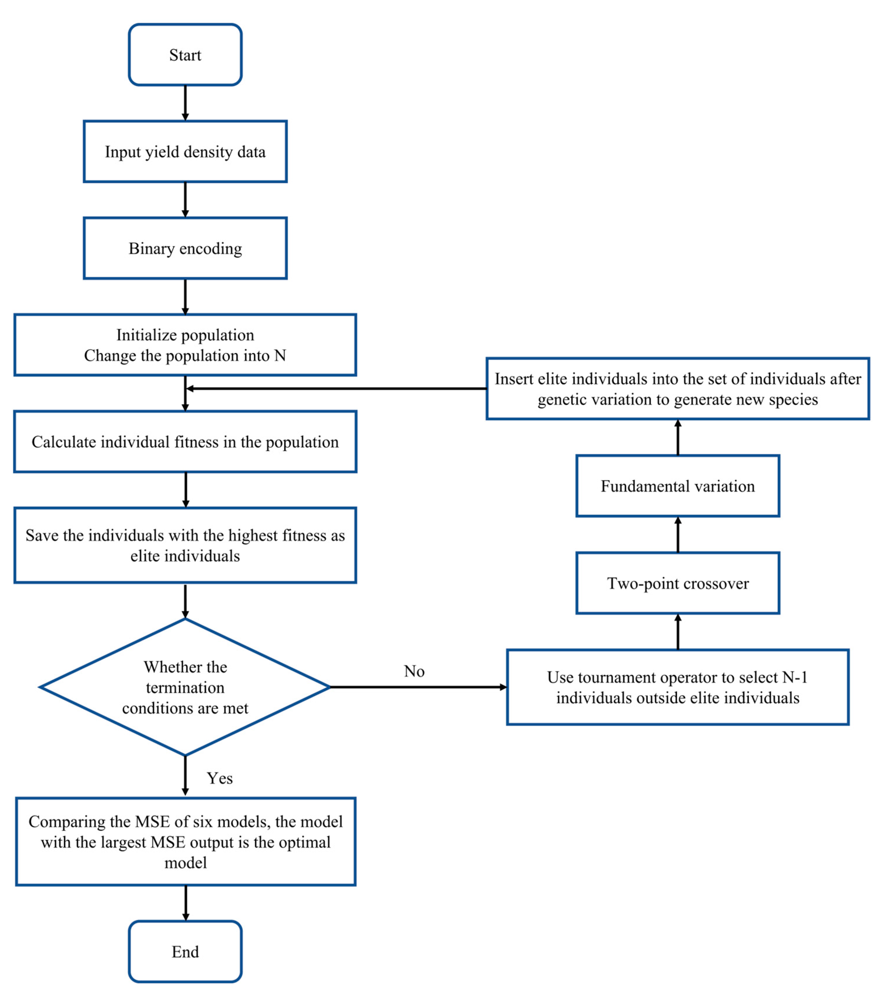
The model parameter estimation and model screening method based on the EGA (Evolutionary Genetic Algorithm) in this study is based on the Python evolutionary algorithm toolbox Geatpy. The toolbox is used to define the problem class for each yield–density model. The least-squares method is used to define the objective function of each yield–density model. The optimization method is used to find the minimum value, and the type of decision variable is a continuous variable. For convenience, the order of the model is adjusted. Geatpy supports calling algorithm templates to realize the rapid implementation of the genetic algorithm and also supports modifying the underlying code to meet different problem requirements. In this study, the genetic algorithm with an elite retention strategy is used for parameter estimation. The coding method is binary, the population size is 200, the individual is selected by using the tournament operator, the two-point crossover is carried out with a crossover probability of 0.7, the basic bit mutation is carried out with a mutation probability of 0.2, and the maximum iteration times are set.
The steps for model parameter estimation and model screening using the EGA (Evolutionary Genetic Algorithm) are shown in Figure 3:
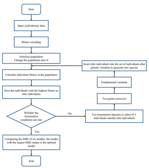
Figure 3.
Parameter estimation and model selection based on EGA.
2.7. CPDOS Solves the Optimum Planting Density Range for the Highest Economic Benefit of Crops
After determining the optimal yield–density model, the economic yield of crops was obtained by using crop yield minus production cost. Then, the optimal planting density range was calculated via a graphical method, and the intersection equation was solved using the dichotomy. The practicability and reliability of the method are verified through an example.
2.7.1. Economic Benefit Yield of CPDOS Crops
The models to be selected, such as Equations (4), (6), (8), (13) and (15), have been able to obtain the maximum value, that the population yield may reach and the corresponding planting density, , but what is required is not the maximum yield and the optimal planting density in reality. Because in the production of crops there will be some production costs, (plant protection, planting operations, etc.), these production costs will also increase with an increase in planting density, so from the perspective of economic benefits, it is necessary to consider the economic benefits of crops. Yield, that is, the maximum value of harvest yield minus the production costs, is the maximum economic yield of crops, and the corresponding planting density is the optimal planting density.
The relationship between production costs, and planting, can be expressed as [12]
The economic benefit yield, is obtained by subtracting the production cost from the harvest yield, which can be expressed as
Through Equation (18), the maximum economic benefit yield, and the corresponding optimum planting density, can be obtained.
2.7.2. Solution Method of Optimum Planting Density Range for Highest Economic Benefit of Crops
In order to achieve the aim of guiding agricultural production, it is obviously easier to give the most suitable planting density range than to give only the most suitable planting density. Therefore, this study sought to determine the most suitable planting density range for the highest economic efficiency. As field operations are often prone to various errors, the sensitivity of field trials is difficult to detect, and the difference between treatments was of less than 5% significance. Therefore, letting the non-significant difference between and be D (this D value can be expressed by 5% ), the most suitable planting density range needs to meet
When finding the most suitable planting density range, the range interval is generally foreseeable, and for the convenience of this study, the graphical method will be used to solve the equation below. The steps for solving the optimal planting density are mainly divided into determining the most economically beneficial yield–density model, determining the graphic method to use to solve the double-intersection equation of the optimal planting density range, and using the dichotomy to solve the equation.
- (1)
- Determining the economic yield–density model
The economic benefit yield is the difference between The harvest yield and production cost. To determine The economic benefit yield, it is necessary to determine harvest yield model and production cost model. Firstly, the EGA (Evolutionary Genetic Algorithm) model parameter estimation and model screening method are used to select the best yield–density model for matching the input yield–density data. Secondly, the EGA (Evolutionary Genetic Algorithm) model parameter estimation method is used to solve the value of parameter p in Equation (17), and then the economic benefit yield model can be obtained by subtracting the two. Taking Equation (2) as an example, the form of the economic benefit yield model obtained is
- (2)
- The optimum planting density range double-intersection equation
Letting one can obtain the optimal planting density, and from Equation (2). The single-intersection equation for solving is
Then the non-significant difference between and is solved, and the double-intersection equation for solving the optimal planting density range is
- (3)
- Dichotomy for solving intersection equation
The basis for solving the intersection equation using the dichotomy is the zero point theorem. The specific calculation steps are as follows:
Step 1: Given the accuracy, determine the equation to be solved, and given the equation zero interval. verify .
Step 2: Find the midpoint, of interval .
Step 3: Calculate .
➀ If then is the zero point of the intersection equation.
➁ If let
➂ If let
If condition 1 is not met, repeat steps 2 and 3 until satisfied.
Before using the dichotomy to solve the intersection equation, we first need to determine the interval where the zero point of exists. The number of intervals required to calculate the single-intersection equation and the double-intersection equation is different, and the double-intersection equation requires two zero intervals. This paper focuses on the determination method of two zero interval of double-intersection equation. The specific steps are as follows:
Step 1: Create an arithmetic sequence, , of planting density, using the numpy.linspace function. It should be noted that: (1) The initial value of the arithmetic sequence is set to 0.01, which is to avoid the occurrence of division 0. (2) The last value of the arithmetic sequence is three times the maximum planting density, in the input data, which is an empirical value, mainly to expand the search range of zeros and avoid zeros outside the set interval.
Step 2: Let traverse find to make let .
Step 3: Traverse the remaining find to make let . The intervals where the two zeros are located are and respectively.
2.8. Optimization of Fertilization Ratio of Planting Density for Maximum Crop Yield by CPDOS
Planting density and fertilizer application are the key factors affecting crop yield and quality. A reasonable fertilization and planting density play an important role in improving yield, controlling production cost, improving economic efficiency, and protecting ecological environment [32,33,34]. The CPDOS uses a BP neural network to fit the data on fertilizer rate and density and uses the genetic algorithm to optimize, trying to find the ratio of fertilizer rate and planting density to maximize yield. Because the CPDOS using BP neural network model fitting requires a large amount of data, in order to make sure that users with less data can also use the system, this study also uses polynomial regression model fitting and optimization to meet the different needs of users.
2.8.1. BP Neural Network Structure Design of CPDOS
In terms of the design of the BP neural network structure, it is mainly divided into the design of the network layer number and the design of the node number of each layer.
- (1)
- Network layer design
In the face of nonlinear problems, the three-layer BP neural network is generally used, that is, the neural network structure of the input layer, the hidden layer, and the output layer. This structure has the advantages of a simple structure, fast data processing speed and short training time and can solve most of the nonlinear problems encountered [35]. The relationship between planting density, fertilization amount, and yield is a nonlinear relationship. Therefore, based on the advantages of the above network structure, when fitting the data on yield, planting density, and fertilization amount based on the BP neural network, a three-layer neural network structure with one input layer, hidden layer, and output layer is selected.
- (2)
- The node number design of each layer
The number of neurons in the input layer is determined by the factors affecting the yield. The influencing factors of this study include planting density and fertilization amount. The fertilization amount mainly includes N fertilizer, P fertilizer, and K fertilizer, and a few experiments also include organic fertilizer. Therefore, the number of nodes in the input layer neurons is determined by the planting density, fertilization amount, and yield data input by the user, and the number is 4 or 5. The BP neural network outputs the predicted value of the yield, so the output layer neuron node number is 1.
The number of hidden layer neuron nodes is of great significance to the BP neural network model. Whether its number is reasonable or not directly affects the fitting ability of the BP neural network model and then affects the accuracy of the model calculation results. Therefore, it is necessary to determine a reasonable number of hidden layer neuron nodes. The formula for determining the number of hidden layer neuron nodes is
In the formula, is the number of hidden layer nodes, is the number of input layer nodes, is the number of output layer nodes, and is the empirical value (). After the calculation, the number of hidden layer neuron nodes ranges from 4 to 12. Through the network model test, the number of hidden layer nodes is determined to be 8.
2.8.2. Data Normalization Processing
The normalization of data can eliminate the dimensional effects of input data and output data, prevent the input signal from being too large, lead to network output saturation, and improve the efficiency of model training. Therefore, before the BP (Back Propagation) neural network training, the data set needs to be normalized. The normalized processing formula is
where is the th datum in the dataset, is the normalized data, the normalized interval is is the minimum value of the th input in the dataset, and is the maximum value of the th input in the dataset.
The inverse normalization formula of Formula (24) is
2.8.3. Cross-Validation
Under the condition of sufficient sample data, a simple method of BP (Back Propagation) neural network model selection is to randomly divide the data set into three parts: training set, verification set, and test set. The training set is used to train the BP model, the validation set is used to select the model with the minimum prediction error, and the test set is used to evaluate the learning method. However, in many practical applications, the amount of data is often insufficient. In order to better model the selection, cross-validation methods can be used. The basic idea of cross-validation is to use data repeatedly: segment the given data, combine the segmented data sets into training sets and test sets, and perform repeated training, testing, and model selection on this basis.
In the study of planting density, fertilizer application, and yield data fitting, due to the long period and large area of field experiments, there are often less experimental data. Therefore, this paper uses a K-fold cross-validation method to deal with the situation of less experimental data.
2.8.4. The Realization of BP Neural Network
The BP neural network is implemented by using the Python deep learning framework PyTorch. The main implementation steps are as follows:
- (1)
- The neural network model structure is determined to be a three-layer BP neural network. The activation functions of the hidden layer and the output layer are Sigmoid functions, and the number of hidden layer neurons is 8.
- (2)
- Use the KFold method in Sklearn to implement K-fold verification, and the K value is set to 5.
- (3)
- Normalize the input data, the normalized interval is .
- (4)
- Setting the model training parameters: using the batch gradient descent method, set the batch size to 10; set the loss function as the mean square error MSE of the predicted value and the true value. Using the Adam optimization method, the initial learning rate is found to be 0.1; set the maximum number of iterations to 10,000; the training termination condition is that the average prediction error of 5 test sets for the maximum number of iterations or cross-validation is less than 0.0002.
- (5)
- BP neural network training, output the best model.
3. Results
3.1. CPDOS Optimal Yield–Density Model
In this study, the genetic algorithm with an elite retention strategy was used for parameter estimation. The coding method was binary, the population size was 200, the individual was selected by the tournament operator, the two-point crossover was performed with a crossover probability of 0.7, and the basic bit mutation was conducted with a mutation probability of 0.2. The maximum number of iterations was 10,000. Following the parameter estimation of the six models, the models were screened according to the MSE.
Mo Huidong believes that the yield–density data conforms to the progressive yield–density relationship and therefore uses the progressive yield–density model formula in Table 3 to fit the data. The EGA (Evolutionary Genetic Algorithm) and sample estimation methods in his paper are used to compare the progressive yield–density model fitting results. The results are presented in Table 4.
Table 4.
Comparison of model fitting results in equation.
As shown, the accuracy was greatly improved when using the EGA (Evolutionary Genetic Algorithm) method for parameter estimation. Both the mean square error, MSE, and the coefficient of determination, were highly optimized. The mean square error (MSE) was reduced by 24.77% compared with Mo Huidong’s fitting result, and the coefficient of determination increased by 1.85%. This demonstrates the effectiveness of using the EGA (Evolutionary Genetic Algorithm) method for parameter estimation.
Table 5 contains the fitting results of the six yield–density models selected using the EGA method.
Table 5.
Fitting results of the model to be selected.
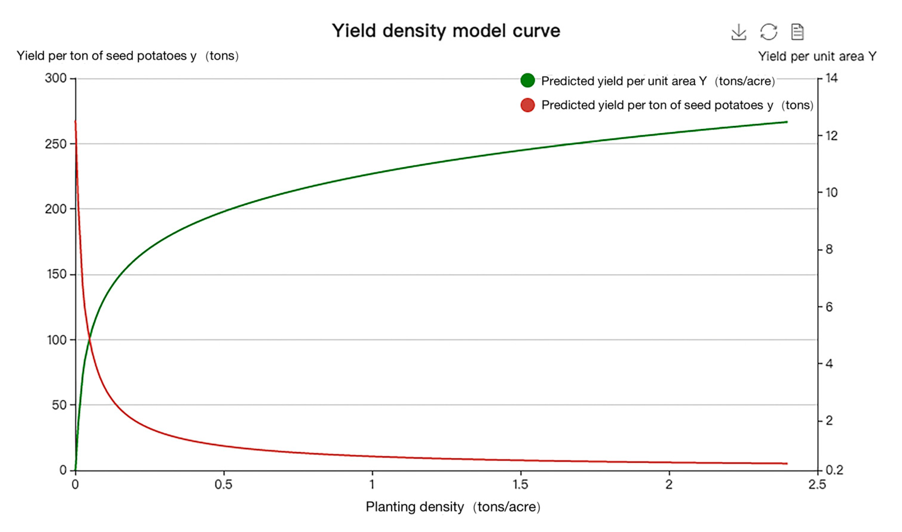
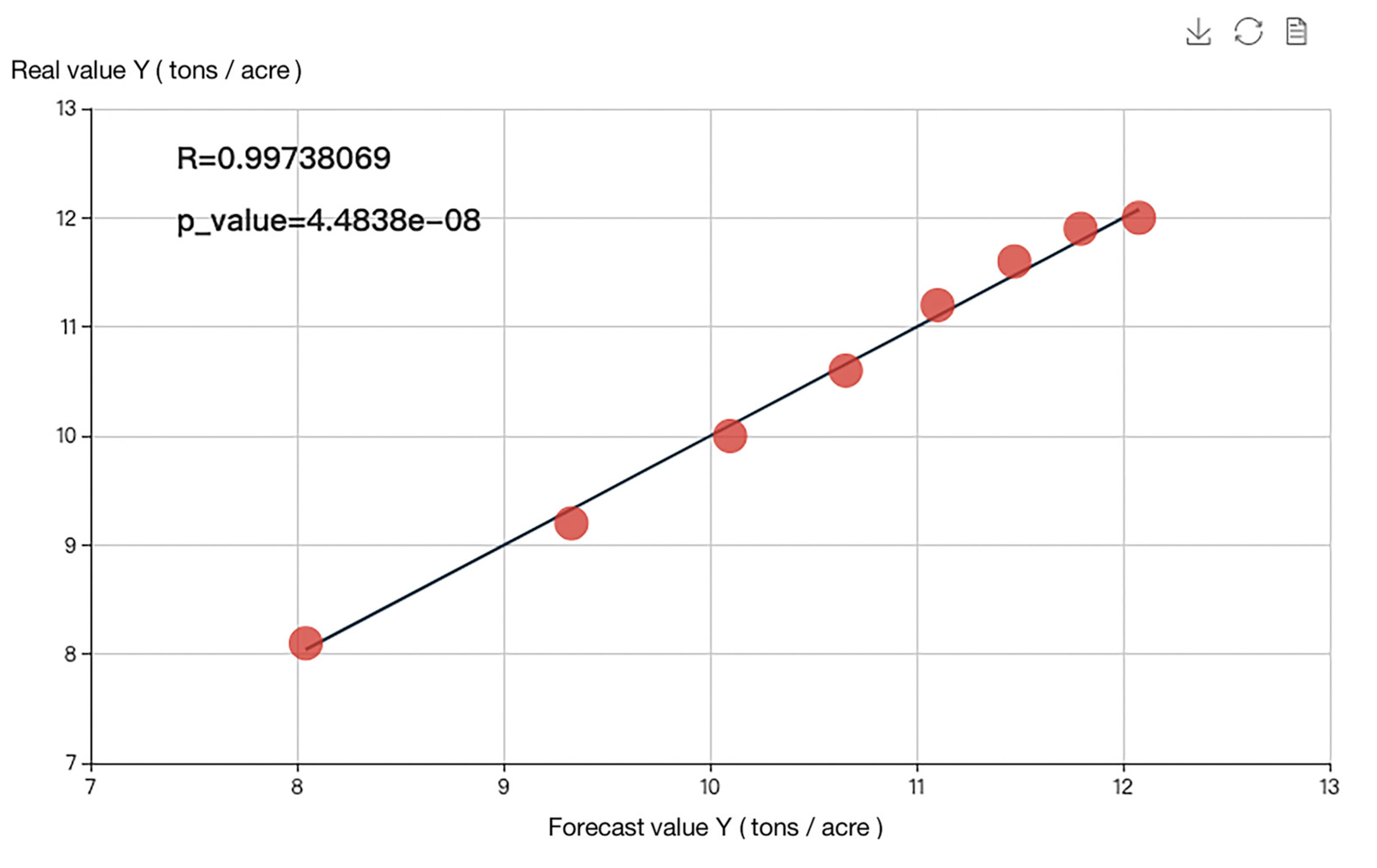
According to the principle of the minimum mean square error, MSE, mixed yield–density model III was the optimal yield–density model matching the relevant data set. The MSE was 0.010813, which is 91.48% lower than Mo Huidong’s fitting result, and the coefficient of determination was 0.994768, which is 6.99% higher. This demonstrates that the use of the EGA (Evolutionary Genetic Algorithm) method for parameter estimation and model screening is both feasible and effective. The optimal yield–density model and goodness-of-fit graphs are all shown in Figure 4 and Figure 5.
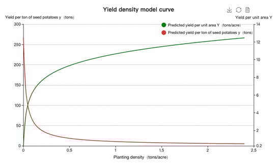
Figure 4.
Curve of the optimal yield–density model for potato based on Mo Huidong.
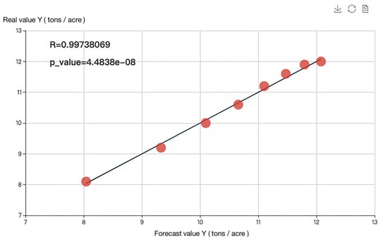
Figure 5.
Goodness-of-fit test chart of optimal yield–density model for potato based on Mo Huidong.
3.2. The CPDOS Optimum Planting Density Range
The cost of crop planting was considered in this paper and the economic crop yield equation was obtained. Using a genetic algorithm to calculate the optimal yield–density and production cost eq.
The EGA-based model fitting results are presented in Table 6.
Table 6.
Fitting results of EGA model.
Mo Huidong selected model II, for the function fitting, while the EGA-based model selection considered model IV, as the best model to match the existing data. The model selection results based on the EGA (Evolutionary Genetic Algorithm) and Mo Huidong’s original method are shown in Table 7.
Table 7.
Comparison of model fitting results.
It was found that the model selected based on the EGA (Evolutionary Genetic Algorithm) method was highly optimized both in the mean square error (MSE) and the coefficient of determination . The mean square error MSE was reduced by 61.0195% compared with Mo Huidong’s original method and the coefficient of determination increased by 5.0501%. This further demonstrates the reliability and practicability of the EGA-based model screening.
The production cost function was fitted by EGA (Evolutionary Genetic Algorithm), the p value was 520.527661, and the mean square error MSE was 76.599768. Therefore, the economic yield–density model can be obtained as
The single-intersection equation that can determine the optimal planting density is
The optimum planting density, and the corresponding maximum economic benefit yield, were obtained via the dichotomy. The double-intersection equation for solving the optimal planting density range was obtained by calculating the difference, of the highest economic benefit yield, without a significant difference:
After using the dichotomy to solve Equation (28), the upper and lower limits of the most suitable planting density range were calculated, which were and respectively. Finally, the optimum planting density range was which was based on the standard of . The diagram of the double-intersection equation graphical method is shown in Figure 6.
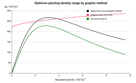
Figure 6.
Schematic diagram of graphic method of double-intersection equation for maize based on Mo Huidong.
3.3. Optimum Fertilization Ratio of Planting Density for CPDOS
The weight matrix, between the input layer and the hidden layer of the BP neural network trained by CPDOS was
The Threshold, of the hidden layer was
The weight matrix, from the hidden layer to the output layer and the threshold of the output layer were
The root mean square error (RMSE) of the BP neural network was 29.2586, and the coefficient of determination was 0.9790. This shows that the use of the BP (Back Propagation) neural network for fitting has high accuracy and can better reflect the functional relationship between planting density, fertilization, and yield. The BP (Back Propagation) neural network goodness-of-fit test is displayed in Figure 7:
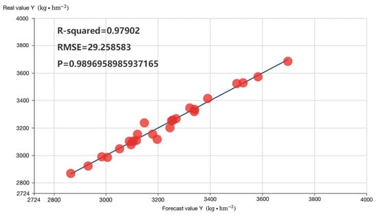
Figure 7.
BP Neural Network goodness-of-fit test chart for soybean based on Liang Xuguang.
3.4. Optimal Yield–Density Model for Different Crops
The optimal yield–density model for different crops can be obtained via the CPDOS, and the yield–density data of the maize in Table 2 are taken as an example. Other examples include the potato crop yield–density data in Table S1; the sorghum crop yield–density data in Table S2; the pepper crop yield–density data in Table S3; the peanut crop yield–density data in Table S4; the sesame crop yield–density data in Table S5; the wheat crop yield–density data in Table S6; and the soybean yield–density data in Table S3. We used the above method to simulate and analyze the table data, screened the model according to the principle of minimum mean square error (MSE), and matched the optimal yield–density model of the current crop yield–density dataset. The best yield–density model fitting results for different crops are presented in Table 8.
Table 8.
Fitting results of optimal yield–density models for different crops.
4. Discussion
4.1. Adaptability of Six CPDOS Classical Yield–Density Models to Crop Species
Previous studies have explored the relationship between crop yield and planting density, but most have not verified the adaptability of a yield–density model to crop species [36]. At the same time, due to the complex parameter estimation problems of these models, they have not been applied in a large number of practical applications. The CPDOS is based on the six classical yield–density models summarized by Mo Huidong. The basic properties and corresponding biological significance of each model were discussed and studied. Subsequently, the genetic EGA (Evolutionary Genetic Algorithm) of the elite retention strategy was used to creatively estimate the model parameters, and the mean square error (MSE) was used as the model selection criterion. The model with the smallest mean square error was selected as the best yield–density model to match the existing dataset. Mo Huidong’s sample estimation of potato yield–density data resulted in an MSE of 0.126897 and a decision coefficient ( of 0.925217 via a custom method. However, our CPDOS system used the EGA (Evolutionary Genetic Algorithm) method for parameter estimation, with a minimum MSE value of 0.010813, which is 91.48% lower than Mo Huidong’s fitting results. The decision coefficient (R2) was 0.994768, an increase of 6.99%. Mo Huidong’s sample estimation of maize yield–density data resulted in an MSE of 133.691331 and a decision coefficient of 0.923564. However, our CPDOS system used the EGA (Evolutionary Genetic Algorithm) method for parameter estimation with a minimum MSE value of 52.113569, which is 61.0195% lower than Mo Huidong’s fitting result. The decision coefficient was 0.970205, an increase of 5.0501%. The adaptability of the model to crop species was greatly improved. However, the six classical yield–density models used in this paper were the same models summarized by researchers more than 50 years ago. A variety of yield–density models should be added in subsequent studies for a comparative analysis and optimization applications to improve the adaptability of the CPDOS.
4.2. Having Additional Comprehensive Crop Production Data Is an Important Basis for Improved CPDOS
The data required to apply the CPDOS is difficult to obtain and the yield–density model optimization and a study of the optimal planting range require stepwise crop planting density data [30]. If the CPDOS is used to optimize the yield–density model, it is advisable to select at least four crop yield sets and crop planting density data from recent years. If the CPDOS is used to calculate the optimal planting range, it is recommended to select four or more crop yield groups, planting density, and total production cost (the sum of various operating costs and material costs during crop production) from recent years and convert them into maize yield consumption data in the production process according to the crop unit price. However, this paper does not consider the impact of environmental, genetic, and other related factors when studying the relationship between yield and density, resulting in a slight deviation between the CPDOS-calculated results and the actual production results [37]. In subsequent research, we would focus on considering such factors to develop a mechanistic model, which would be combined with the existing yield–density model to optimize crop planting density and improve the applicability and accuracy of the CPDOS. At the same time, if new yield–density models and mechanistic models are added, the system would require significantly more local crop growth data, including temperature, precipitation, soil fertility, and genetics [38]. The addition of crop growth data is conducive to improving the applicability and accuracy of the CPDOS globally, helping global agricultural researchers to analyze data and guide agricultural production while playing an important role in the development of future agricultural intelligent systems.
4.3. The CPDOS System Still Has Significant Room for Improvement
When constructing systems, the CPDOS chooses steps to simplify any complexity, uses available development space, and improves functions. So far, the crop planting density optimization system has been released on the Ali cloud server. With wider and evolving research, many new functions and methods will be successfully added, and the existing module functions will be improved. The improvement of the function module can be approached from two perspectives: (1) Select more stable and searchable optimization methods, such as hybrid heuristic optimization algorithms. (2) Study the data augmentation method for regression problems. Yield–density model studies often only collect a small amount of data. The study of data augmentation methods for regression problems can improve the yield–density model fitting accuracy and reduce the limitations of using the neural network method.
5. Conclusions
In order to optimize crop planting density and obtain noteworthy research results, a crop planting density optimization system based on modern computing technology and network information technology was designed. The CPDOS mainly uses the EGA (Evolutionary Genetic Algorithm), dichotomy, polynomial regression, and a BP neural network. The two core functions of the system are model parameter estimation and model selection based on a genetic algorithm and the optimal planting density calculation. Six renowned crop planting density optimization models were included in the present study, and an elite retention strategy was employed to solve the complex parameter estimation problems of the models. Through such means, issues were effectively resolved, and the applicability of the models was expanded. The CPDOS comprises three core modules: yield–density optimization module, optimal planting density range module, and fertilization and planting density optimization module. By using the proposed system, users can better analyze the existing yield–density data and other data. The proposed system also simultaneously facilitates the optimization of both planting density and the allocation of fertilization and planting density.
Supplementary Materials
The following supporting information can be downloaded at: https://www.mdpi.com/article/10.3390/agronomy13102465/s1, Table S1: Potato yield density data of Wang Kui. Table S2: Sorghum yield density data of Ni Yuqiong. Table S3: Red Pepper yield density data of XinBin. Table S4: Peanut yield density data of Huang Xiujun. Table S5: Sesame yield density data of Huang Zhou Linna. Table S6: Wheat yield density data of Zhang Shibao. Table S7: Soybean yield density data of Li Xiaoyu. Figure S1: Registration interface of crop planting density optimization system. Figure S2: Login interface of crop planting density optimization system. Figure S3: Display of optimization results of yield density model. Figure S4: Data table visualization. Figure S5: Curve chart of optimal yield density model. Figure S6: Goodness of fit test chart of optimal model. Figure S7: Display page of calculation results of optimum planting density range. Figure S8: Data table display page. Figure S9: Graphical Method Schematic Display Page. Figure S10: Optimal yield density model curve diagram and goodness of fit test diagram. Figure S11: Progressive yield density relation curve. Figure S12: Yield density relation curve proposed by Fan Furen and Mo Huidong. Figure S13: Curve of quadratic model. Figure S14: Yield density curve of mixed type.
Author Contributions
Z.Z. (Zhixin Zhang): Software, Data curation, Writing—original draft preparation, Visualization, Writing—original draft, Writing—review and editing. Y.C.: Methodology, Software, Visualization, Investigation. Z.H.: Investigation, Supervision. Y.L.: Data curation, Supervision. H.C.: Visualization, Supervision. Z.Z. (Zhenqing Zhao): Methodology, Supervision. D.X.: Writing—review and editing. Q.C.: Writing—review and editing, Supervision. R.Z.: Conceptualization, Methodology, Investigation, Writing—review and editing, Supervision. All authors have read and agreed to the published version of the manuscript.
Funding
The authors acknowledge the financial supports of the National Key Research and Development Program of the “14th Five Year Plan” (Accurate identification of yield traits in soybean) (2021YFD120160204), Research and Application of Key Technologies for Intelligent Farming Decision Platform, An Open Competition Project of Heilongjiang Province, China (2021ZXJ05A03), and the Natural Science Foundation of Heilongjiang Province of China (LH2021C021).
Data Availability Statement
The data presented in this study are available on request from the corresponding author. The data are not publicly available because the data need to be used in future work.
Conflicts of Interest
The authors declare that they have no known competing financial interest or personal relationships that could have appeared to influence the work reported in this paper.
References
- Lv, X. Review of mid-and long-term predictions of China’s grain security. China Agric. Econ. Rev. 2013, 5, 567–582. [Google Scholar] [CrossRef]
- Chen, Y.; Li, X.; Wang, J. Changes and effecting factors of grain production in China. Chin. Geogr. Sci. 2011, 21, 676–684. [Google Scholar] [CrossRef]
- Khan, A.; Najeeb, U.; Wang, L.; Tan, D.K.Y.; Yang, G.; Munsif, F.; Ali, S.; Hafeez, A. Planting density and sowing date strongly influence growth and lint yield of cotton crops. Field Crops Res. 2017, 209, 129–135. [Google Scholar] [CrossRef]
- Willey, R.W.; Heath, S.B. The quantitative relationships between plant population and crop yield. Adv. Agron. 1969, 21, 281–321. [Google Scholar] [CrossRef]
- Holliday, R. Plant population and crop yield. Nature 1960, 186, 22–24. [Google Scholar] [CrossRef]
- Shinozaki, K. Intraspecific competition among higher plants. VII. Logistic theory of the CD effect. J. Inst. Polytech. Osaka City Univ. Ser. 1956, 7, 35–72. [Google Scholar]
- Fang, X.; Li, Y.; Nie, J.; Wang, C.; Huang, K.; Zhang, Y.; Zhang, Y.; She, H.; Liu, X.; Ruan, R.; et al. Effects of nitrogen fertilizer and planting density on the leaf photosynthetic characteristics, agro-nomic traits and grain yield in common buckwheat (Fagopyrum esculentum M.). Field Crops Res. 2018, 219, 160–168. [Google Scholar] [CrossRef]
- Zhou, C.; Huang, Y.; Jia, B.; Wang, Y.; Wang, Y.; Xu, Q.; Li, R.; Wang, S.; Dou, F. Effects of cultivar, nitrogen rate, and planting density on rice-grain quality. Agronomy 2018, 8, 246. [Google Scholar] [CrossRef]
- Tang, K.; Struik, P.; Yin, X.; Calzolari, D.; Musio, S.; Thouminot, C.; Bjelková, M.; Stramkale, V.; Magagnini, G.; Amaducci, S. A comprehensive study of planting density and nitrogen fertilization effect on dual-purpose hemp (Cannabis sativa L.) cultivation. Ind. Crops Prod. 2017, 107, 427–438. [Google Scholar] [CrossRef]
- Shahzadi, R.; Ferzund, J.; Tausif, M.; Suryani, M.A. Internet of things based expert system for smart agriculture. Int. J. Adv. Comput. Sci. Appl. 2016, 7, 341–350. [Google Scholar] [CrossRef]
- Hu, X.; Qian, S. IoT application system with crop growth models in facility agriculture. In Proceedings of the 2011 6th International Conference on Computer Sciences and Convergence Information Technology (ICCIT), Seogwipo, Republic of Korea, 29 November–1 December 2011; pp. 129–133. [Google Scholar]
- Mo, H. Planting density and crop yield-an analysis of quantitative relationships between yield and density. Acta Agron. Sin. 1980, 6, 65–74. [Google Scholar]
- Liang, X.-g.; Wang, F.-l.; Zhao, H.-l.; Dong, Z.-G. Optimization of Soybean Planting Density and Fertilizer Application Rate Based on RBF Neural Network. Soybean Sci. 2020, 39, 406–413. [Google Scholar] [CrossRef]
- Wang, K.; Fang, Y.; Jing, M.; Sun, L. Effects of Different Planting Densities on Yield of Qingshu 9 in Yulin Water-land. Shaanxi Agric. Sci. 2015, 61, 7–9+18. [Google Scholar]
- Ni, Y.; Zhang, Q. Effects of Different Planting Density on Yield of Wine Sorghum. Agric. Dev. Equip. 2015, 9, 74–76. [Google Scholar]
- Xin, B.; Wang, L.; Zou, C. Effect of Different Planting Densities on Yield of Red Pepper in Beipiao Area. Pepper Mag. 2015, 13, 16–18. [Google Scholar]
- Huang, X.; Bi, J.; Zhang, X. Effects of different planting density on peanut yield. Agric. Technol. 2018, 38, 14–15. [Google Scholar]
- Zhou, L.; Zhou, X.; Shi, M.; Cui, X.; Kan, Y.; Wang, X.; Cui, J.; Zhu, Y. Effects of different planting densities of sesame on its biological characteristics. Bull. Agric. Sci. Technol. 2015, 9, 162–164. [Google Scholar]
- Zhang, S.; Nong, M.; Gao, H.; Nong, C.; Wang, X.; Zhao, K.; He, J. Effects of different ni-trogen application rates and planting densities on agronomic traits and yield of Wenmai 14. South. Agric. 2021, 15, 31–32+39. [Google Scholar] [CrossRef]
- Li, X.; Li, X.; Zhang, D.; Li, X.; Kang, Y.; Wu, X. Effect of Different Planting Densities on Yield of New Soybean Variety Kaidou. Bull. Agric. Sci. Technol. 2020, 46, 152–154. [Google Scholar]
- Fan, F.R.; Mo, H.D.; Ching, T.C.; Hu, X.H. Studies on the planting rate of corn. Acta Agron. Sin. 1963, 2, 381–398. [Google Scholar]
- Duncan, W.G. The relationship between corn population and yield 1. Agron. J. 1958, 50, 82–84. [Google Scholar] [CrossRef]
- Carmer, S.G.; Jackobs, J.A. An Exponential Model for Predicting Optimum Plant Density and Maximum Corn Yield 1. Agron. J. 1965, 57, 241–244. [Google Scholar] [CrossRef]
- Farazdaghi, H. Some Aspects of the Interaction between Irrigation and Plant Density in Sugar Beets. Ph.D. Thesis, University of Reading, Reading, UK, 1968. [Google Scholar]
- Ding, C. The theoretical curve equation of density-yield and its discussion. Shanghai Agric. Sci. Technol. 1978, 14, 4–9+26. [Google Scholar]
- Bleasdale, J.K.A.; Nelder, J.A. Plant population and crop yield. Nature 1960, 188, 342. [Google Scholar] [CrossRef]
- Hudson, H.G. Population studies with wheat: III. Seed rates in nursery trials and field plots. J. Agric. Sci.-Ence 1941, 31, 138–144. [Google Scholar] [CrossRef]
- Stanger, T.F.; Lauer, J.G. Optimum plant population of Bt and non-Bt corn in Wisconsin. Agron. J. 2006, 98, 914–921. [Google Scholar] [CrossRef]
- Coulter, J.A.; Nafziger, E.D.; Janssen, M.R.; Pedersen, P. Response of Bt and near-isoline corn hybrids to plant density. Agron. J. 2010, 102, 103–111. [Google Scholar] [CrossRef]
- Van Roekel, R.J.; Coulter, J.A. Agronomic responses of corn to planting date and plant density. Agron. J. 2011, 103, 1414–1422. [Google Scholar] [CrossRef]
- Assefa, Y.; Prasad, P.V.V.; Carter, P.; Hinds, M.; Bhalla, G.; Schon, R.; Jeschke, M.; Paszkiewicz, S.; Ciampitti, I.A. Yield responses to planting density for US modern corn hybrids: A synthesis-analysis. Crop Sci. 2016, 56, 2802–2817. [Google Scholar] [CrossRef]
- Ren, X.-J.; Lv, X.-Y.; Ma, J.-K. Effects of Different Planting Densities and Fertilization Levels on Yield and Main Agro-nomic Characters of Early-maturing Summer Soybean in Shanxi Province. Soybean Sci. 2019, 38, 921–927. [Google Scholar] [CrossRef]
- Yang, J.; Huang, S.; Yang, M. Effect of density and fertilizer amount on yield of different branching types of soybeans. Soybean Sci. 2012, 32, 382–384. [Google Scholar] [CrossRef]
- Muoneke, C.O.; Ogwuche, M.A.O.; Kalu, B.A. Effect of maize planting density on the performance of maize/soybean intercropping system in a guinea savannah agroecosystem. Afr. J. Agric. Res. 2007, 2, 667–677. [Google Scholar]
- Zhang, X.; Wang, Q.; Huo, Z.; Yu, T.; Wang, G.; Liu, T.; Wang, W. Prediction of frost-heaving behavior of saline soil in western jilin province, china, by neural network methods. Math. Probl. Eng. 2017, 2017, 7689415. [Google Scholar] [CrossRef]
- Cousens, R. A simple model relating yield loss to weed density. Ann. Appl. Biol. 1985, 107, 239–252. [Google Scholar] [CrossRef]
- Hristov, N.; Mladenov, N.; Kondić-Špika, A.; Jeromela, A.M. Effect of environmental and genetic factors on the correlation and stability of grain yield components in wheat. Genet. Belgrade 2011, 43, 141–152. [Google Scholar] [CrossRef]
- Childs, S.W.; Hanks, R.J. Model of soil salinity effects on crop growth. Soil Sci. Soc. Am. J. 1975, 39, 617–622. [Google Scholar] [CrossRef]
Disclaimer/Publisher’s Note: The statements, opinions and data contained in all publications are solely those of the individual author (s) and contributor (s) and not of MDPI and/or the editor (s). MDPI and/or the editor (s) disclaim responsibility for any injury to people or property resulting from any ideas, methods, instructions or products referred to in the content. |


Disclaimer/Publisher’s Note: The statements, opinions and data contained in all publications are solely those of the individual author(s) and contributor(s) and not of MDPI and/or the editor(s). MDPI and/or the editor(s) disclaim responsibility for any injury to people or property resulting from any ideas, methods, instructions or products referred to in the content. |
© 2023 by the authors. Licensee MDPI, Basel, Switzerland. This article is an open access article distributed under the terms and conditions of the Creative Commons Attribution (CC BY) license (https://creativecommons.org/licenses/by/4.0/).