Article

Machine Learning-Based Processing of Multispectral and RGB UAV Imagery for the Multitemporal Monitoring of Vineyard Water Status

1
Instituto de Desarrollo Regional (IDR), Universidad de Castilla-La Mancha, 02071 Albacete, Spain
2
Department of Ecology, Desertification Research Centre (CIDE-CSIC-UV-GV), 46113 Moncada, Spain
3
Centro de Edafología y Biología Aplicada del Segura, Consejo Superior de Investigaciones Científicas (CEBAS-CSIC), 30100 Murcia, Spain
*
Author to whom correspondence should be addressed.
Agronomy 2022, 12(9), 2122; https://doi.org/10.3390/agronomy12092122
Submission received: 25 July 2022 / Revised: 1 September 2022 / Accepted: 4 September 2022 / Published: 7 September 2022
(This article belongs to the Special Issue Precision Water Management)

Abstract

:
The development of unmanned aerial vehicles (UAVs) and light sensors has required new approaches for high-resolution remote sensing applications. High spatial and temporal resolution spectral data acquired by multispectral and conventional cameras (or red, green, blue (RGB) sensors) onboard UAVs can be useful for plant water status determination and, as a consequence, for irrigation management. A study in a vineyard located in south-eastern Spain was carried out during the 2018, 2019, and 2020 seasons to assess the potential uses of these techniques. Different water qualities and irrigation application start throughout the growth cycle were imposed. Flights with RGB and multispectral cameras mounted on a UAV were performed throughout the growth cycle, and orthoimages were generated. These orthoimages were segmented to include only vegetation and calculate the green canopy cover (GCC). The stem water potential was measured, and the water stress integral (Sψ) was obtained during each irrigation season. Multiple linear regression techniques and artificial neural networks (ANNs) models with multispectral and RGB bands, as well as GCC, as inputs, were trained and tested to simulate the Sψ. The results showed that the information in the visible domain was highly related to the Sψ in the 2018 season. For all the other years and combinations of years, multispectral ANNs performed slightly better. Differences in the spatial resolution and radiometric quality of the RGB and multispectral geomatic products explain the good model performances with each type of data. Additionally, RGB cameras cost less and are easier to use than multispectral cameras, and RGB images are simpler to process than multispectral images. Therefore, RGB sensors are a good option for use in predicting entire vineyard water status. In any case, field punctual measurements are still required to generate a general model to estimate the water status in any season and vineyard.

1. Introduction

The European Union (EU) is the world leader in wine production and had a vine-growing area greater than 3.7 million hectares in 2019; this represents approximately 50% of the global vineyard area [1]. Spain has the largest vineyard area in the world (949,565 ha in 2020), and the area of irrigated vineyards is increasing (from 33% in 2010 to more than 40% in 2020) [2]. Irrigation has a direct impact on vine yield and grape quality [3]. However, irrigation to replenish potential water needs may result in increases in vegetative growth and yield, as well as adverse effects on other parameters associated with quality, such as sugar content, acidity, and pigment synthesis. Thus, optimal irrigation scheduling is a key issue in balancing production and quality.
The water resources available for agricultural uses are very limited due to the increasing competition among the different economic uses of water, environmental limitations, and the effects of climate change. This problem is especially severe in Mediterranean countries, which experience semiarid climate conditions [4]. In this context, water use efficiency and water productivity are highly relevant and are key factors for irrigation sustainability [5]. Thus, in the context of water scarcity, sustainable irrigation management techniques should be applied; these techniques include regulated deficit irrigation (RDI), which is especially useful for woody crops such as grapevines [6]. RDI can also have positive effects on vine quality and yield. The effect of the water deficit, and consequently, the appropriate RDI management approach, depends on the vine phenological growth, plant water stress, and the soil and climatic water conditions [7].
These techniques, similar to other tools improving agricultural water use, require the monitoring of crop water status and its progress over time. Midday stem water potential (Ψstem) has been proposed as a significant physiological indicator of water status for irrigated and rain-fed vines [8,9]. Nevertheless, these measurements are performed manually, are time-consuming, and may not be representative of the spatial variability of the water status over the whole vineyard [10]. Moreover, Ψstem only represents a snapshot of plant water stress at the time of measurement [11]. Additionally, the changes in irrigation depths with time and the lack of uniformity in water application during the irrigation period emphasize the need for a methodology that would cover the entire season, integrating the short-term variations in vine water status. One option would be to use an integrated measure throughout the growing season, known as the water stress integral (Sψ), enabling the analysis of the effect of the cumulative water deficit duration and intensity [12].
Precision viticulture involves optimizing fertilizer, phytochemical, and water application rates to the specific needs of each area in the field [13]. The emergence of precision viticulture was possible when technological advancements concurred, such as the appearance of precise global navigation satellite systems, the development of software designed to analyse geographic data, and the increasing availability of geolocated information remotely acquired [14]. Remote sensing (RS) methods based on spectral vegetation indices (VIs) and infrared thermometry are widely used for crop water stress detection because they are non-destructive and have low labour and time requirements. The most affected process by water stress promoted by high temperatures is net photosynthesis. The stomatal conductance, chlorophyll content, and leaf transpiration rate are also influenced by water stress. The accumulated effect of these physiological parameters is evidenced in the leaf spectral response tracked by RS technologies [15]. Hence, in this study, the canopy spectral response was related to the accumulated effect of water stress through the Sψ.
The use of unmanned aerial vehicles (UAVs) as platforms to obtain aerial imagery has several advantages over the use of satellites, airplanes, balloons, and helicopters, which are traditionally used in RS. UAVs with lightweight, high-quality calibrated geometric and radiometric sensors allow users to obtain data with very high spatial (centimetric spatial resolution) and temporal resolutions, according to user needs. VIs, by mathematically combining spectral reflectance data from onboard sensors, have traditionally been used to monitor biochemical and biophysical attributes of crops. Green canopy cover (GCC), which is representative of the canopy vigour, is another product obtained from aerial imagery used for this purpose [16,17,18,19,20,21]. Vegetation segmentation is required to evaluate the reflectance response of the crop and, therefore, to eliminate the soil effect [22].
The spectral response of the plant to different physiological changes does not always corresponds to linear relations; for this reason, sometimes traditional statistical models are not powerful enough to obtain accurate plant water status estimations [23]. Therefore, artificial intelligence (AI) algorithms are a good alternative to other techniques due to their ability to describe both linear and non-linear systems [10]. Machine learning (ML) is a type of AI that gives machines the ability to learn from relationship between inputs and outputs in the training stage. Its algorithms use an optimization method to calibrate parameters of predetermined equations based on the training datasets. The algorithms progressively adapt to enhance their performance as the available number of training samples increases [24]. ML techniques are constantly undergoing development and are widely applied across almost all fields. However, the main limitation of ML and the statistical models is that they are “site-specific” and “time-specific” [25].
ML has the potential to evolve a real-time farm-specific management system as support to the famer to make appropriate decisions when it is applied to remotely sensed data. Many ML algorithms have been used to detect crop water stress using data acquired from RS. For instance, Pôças et al. [26] used random forest (RF) and support vector machine (SVM) predictive ML models to model predawn leaf water potential to assess water stress in vineyards. Moshou et al. [27] attempted to distinguish between healthy and water-stressed wheat canopies using a developed hybrid classification technique with a multisensory fusion system and a least squares support vector machine (LSSVM) algorithm. Loggenberg et al. [28] applied RF and XGBoost to discriminate between stressed and non-stressed vines. Nevertheless, RF and SVM algorithms are rarely applied for the determination of plant water status. Artificial neural networks (ANNs) are a widely utilized ML technique in water stress detection and other studies in agriculture, and they are good at addressing agricultural issues to which deterministic models cannot be applied [10,29]. Poblete et al. [22] built an ANN model to predict the spatial variability in Ψstem in a vineyard. Romero et al. [23] also used ANN models to predict Ψstem using VIs computed from multispectral imagery. The relative water content, which is another water stress indicator measured based on plant responses, was also predicted under water deficit stress in rice genotypes by Krishna et al. [30] through spectral indices, multivariate techniques, and ANN models. However, none of these studies evaluated the capacity of conventional RGB cameras to predict water stress or compared their capacity with that of multispectral cameras. Although conventional RGB cameras have a poor radiometric quality, the use of RGB cameras would provide many substantial advantages, including (1) RGB cameras are much more affordable than multispectral cameras, (2) the photogrammetry process for RGB information is more robust than that for multispectral sensor data, and (3) the spatial resolution of RGB cameras at the same flight height is much higher.
Therefore, the main objective of this research is to develop ANN models that integrate very high-spatial resolution RGB and multispectral information about the canopy and to compare their performance to predict the water stress of a vineyard. To assess their performance, multiple linear regression models (MRM) were obtained using the same predictor variables as in the ANN models. To obtain a wide range of vine water status conditions, several irrigation strategies were tested during three irrigation seasons, including strategies with different water salinity levels andirrigation application start throughout the growth cycle.

2. Materials and Methods

The methodology used in this experimental study is summarized in Figure 1 and will be detailed in the following subsections.

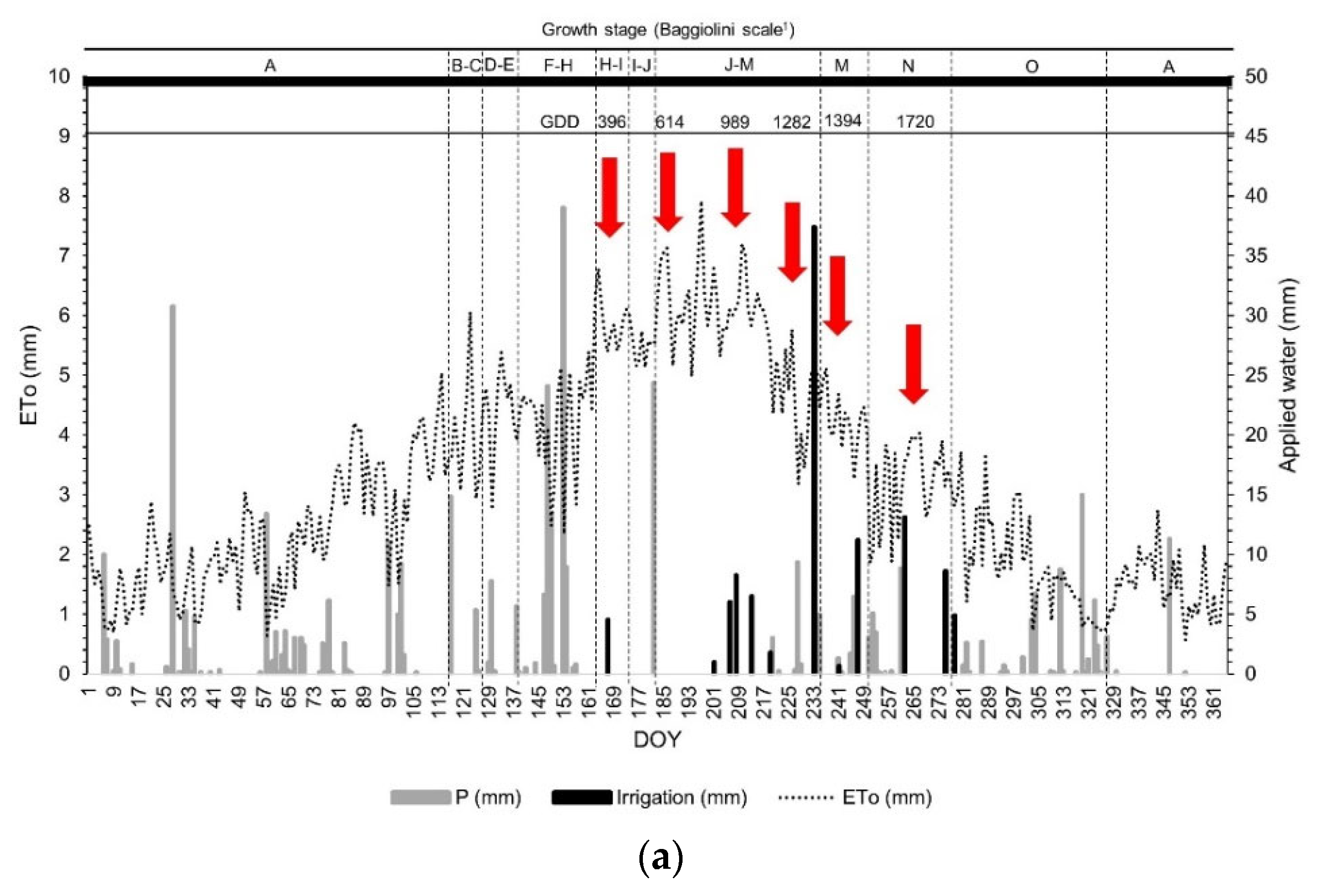
2.1. Study Site and Experimental Design

The field experiment was conducted in a commercial vineyard located in Fuente-Álamo, Albacete, Spain (38°43′43.3″ N, 1°28′12.6″ W; elevation 820 m a.s.l.; see Figure 2) during the 2018, 2019, and 2020 growing seasons. The climate is defined as typical Mediterranean semiarid [31]. Climate data were obtained from a weather station located 10 km from the experimental plot in 2018, and from a weather station located in the experimental plot in the following studied seasons (2019 and 2020). Table 1 shows the annual rainfall and reference evapotranspiration (ET0) data, and those recorded during the growing season (from April to the end of September) for the studied years. There was more rainfall in 2019 and 2020 than in 2018, and in particular more rainfall during the growth stage in 2019, mainly due to torrential rains in April and September. Rainfall was more evenly distributed throughout the 2018 growing season (Figure 3a). In 2019, the ET0 was 8.5% higher than in 2018, and 7.1% higher than 2020. The number of growing degree days (GDD) from April to harvest was computed as the sum of the average daily temperatures above a threshold of 10 °C [32]. Upon harvest (10 October 2018, 7 October 2019, and 29 September 2020, respectively), GDDs were 1904, 1868, and 1836, respectively.
The trial was carried out in a 0.6-hectare subplot of a 6.5-hectare commercial vineyard (Figure 2). Soil was sandy loam (with more than 55% sand) with a variable depth up to 90 cm. Soil had 1.2% organic matter, 47.7% active CaCO3, electrical conductivity (EC) of 0.4 dS/m, pH of 8.9, and bulk density of 1.2 g/cm3. The irrigation water analysis showed an EC of 1.3 dS/m and pH of 8.4. Monastrell vines (grafted onto 110-Richter) were planted in 2007 at a spacing of 3 m × 1.5 m (2222 vines/ha). They were trained to a double Guyot system on a vertical trellis. The vineyard rows were oriented north–south. The inter-row was regularly tilled and the soil under the vine rows was kept weed-free by the use of herbicides. In May, green non-productive shoots were removed from each vine for all treatments. In July, green shoots were trimmed from each grapevine following local growing practices. No fertilisers were applied. Sulphur treatments were applied to flowers and pea-sized berries to prevent fungal diseases. The plot was irrigated with 4 L/h, self-compensating drippers with 1 m spacing. The annual available water for irrigation was set at 1000 m3/ha.
The experimental design consisted of four random blocks. Six treatments (T1–T6) were randomly established in each block (Figure 2). Each experimental unit included four rows of 12 vines. The two outer rows were considered buffers (not considered in the sampling process). The most external vines in every row were also considered as buffers. The treatments consisted of a rain-fed treatment (T1), irrigation with standard-quality water (T2), and four irrigation treatments with added salts reaching an EC of 5 dS/m: T3, T4, T5 and T6 (Table 2). Irrigation began when Ψstem reached −0.8 MPa, except in T5 and T6, which started at veraison. In the 2019 and 2020 seasons, the experimental design was simplified; T5 and T6 were not implemented because differences from the other salt treatments (T3 and T4) in terms of the agronomic characteristics and grape quality were not observed [34].

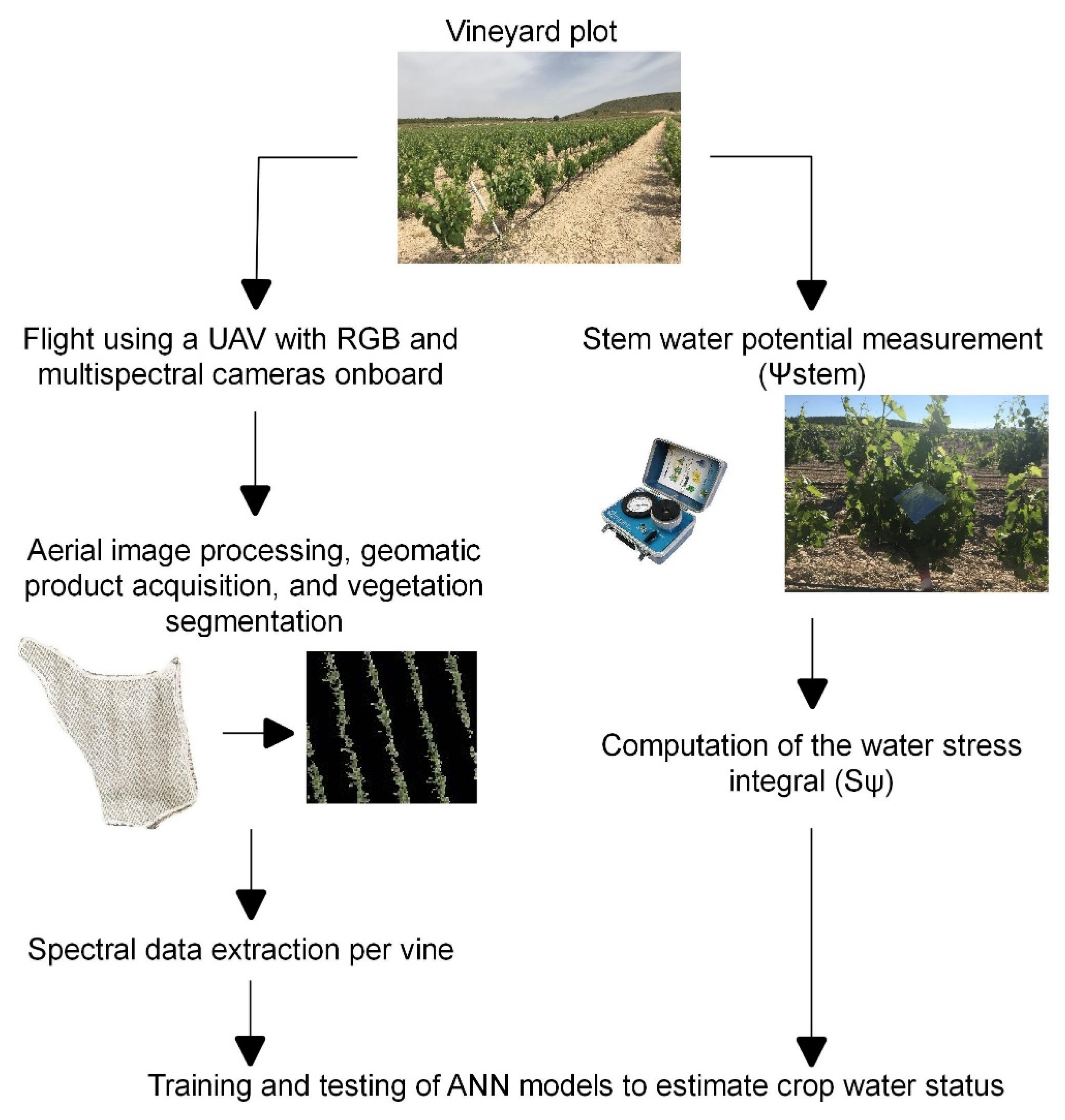
2.2. Plant Water Status Measurements, and Aerial Image Acquisition and Processing

Each year, the grapevine water status was determined at midday (11:30–12:30 solar time) by measuring Ψstem on two representative vines per experimental unit and one leaf per vine, using a pressure chamber (PMS Instrument Company, Albany, OR, USA). Leaves were taken from the west side of the row and were placed in totally hermetic plastic bags covered with aluminium foil for at least 2 h prior to the measurement time, from June to September at fortnightly intervals (Figure 3). The leaves were cut and immediately placed in the chamber. Because of the wide range of irrigation treatments implemented, the vine water statuses of a total of 48 vines were assessed in 2018. In 2019 and 2020, 32 vines were sampled.
Following Myers [35], the effect of water deficit duration and intensity was accounted for by the Sψ computed as the summation of the difference in the average of two consecutive measurements of Ψstem ( ψ ¯ i , i + 1 ) and the least negative value registered during the season (c = −0.35 MPa in 2018 and 2019, and c = −0.28 MPa in 2020), multiplied by the number of days between one measurement and the next (n), as follows:
S φ = | i = 0 i = t ψ ¯ i , i + 1 c n |
Flights at an altitude of 80 m high were carried out during three seasons (six flights in 2018 and seven in 2019 and 2020 seasons) (Figure 1 and Figure 3). All flights and image acquisition were concurrently done with Ψstem field measurements. The flights were always performed near solar noon (between 11:00 and 12:00 solar time) to reduce the grapevine shadow on the images. A multispectral SEQUOIA sensor (Parrot Drone SAS, Paris, France) and an RGB SONY ILCE-5100 digital camera (Sony Corporation, Tokyo, Japan) were mounted on a quadcopter md4-1000 (Microdrones Inc., Kreuztal, Germany). The characteristics of both sensors are shown in Table 3.
Flight planning was performed by using the Microdrones Photogrammetric Flight Planning software (MFLIP) [36]. Eight targets with known coordinates were used to georeference the obtained images and calibrate the cameras geometrically. Radiometric calibration was performed before each flight using the Aircalib calibration panel (Airinov, Paris, France) for the multispectral sensor, to obtain reflectance values. For the RGB camera, the digital levels for each band were obtained and no calibration was performed. The normalisation of RGB bands was performed following the methodology of Woebbecke et al. [37].
Blurred images were automatically detected and eliminated [38] to avoid artefacts during the photogrammetry process. The software Agisoft Metashape Professional (Agisoft LLC, St. Petersburg, Russia), version 1.6.1, was used to perform the photogrammetric process obtaining geomatic products, such as high-resolution multispectral (8-centimetre ground sample distance; GSD) and RGB (2-centimetre GSD) images. These high spatial resolution images allowed us to have a very accurate vegetation cover.
Leaf Area Index Calculation software (LAIC) [39] was used to discriminate GCC from other features (ground, stones, and shadows, among others) in very high spatial resolution aerial images. GCC is a geometric parameter that provides information about vegetative growth status [40]. “GCC” was used to name the GCC from the RGB sensor and “GCCMULTI” to define the GCC obtained from the multispectral sensor. Differences between GCC and GCCMULTI are expected due to the different spatial resolution of the geomatic products. Figure 4 shows the flowchart of the processes implemented with LAIC software in a multispectral orthoimage.
The effect of salt treatments on canopy spectral reflectance was assessed using a test of multiple comparisons (Tukey test) to check the significant differences of the mean values of each band acquired by the sensors for each treatment and season. No significant differences were observed between the different treatments in any sampling events of the three seasons. Therefore, data analysis was conducted for all treatments together.

2.3. Machine Learning Modelling and ANN

ANNs are biologically inspired computer programs designed to simulate the way in which the human brain processes information. ANNs gather their knowledge by detecting the patterns and relationships in data and learn (or are trained) through experience, not from programming. An ANN is formed from hundreds of single units, artificial neurons or processing elements (PE), connected with coefficients (weights), which constitute the neural structure and are organised in layers. The power of neural computations comes from connecting neurons in a network. Each PE has weighted inputs, transfer function, and one output. The behavior of a neural network is determined by the transfer functions of its neurons, by the learning rule, and by the architecture itself. The weights are the adjustable parameters and, in that sense, a neural network is a parameterized system. The weighed sum of the inputs constitutes the activation of the neuron. The activation signal is passed through transfer function to produce a single output of the neuron. Transfer function introduces non-linearity to the network. During training, the inter-unit connections are optimized until the error in predictions is minimized and the network reaches the specified level of accuracy [41]. The NETLAB toolbox in MATLAB software (Mathworks Inc., Natick, MA, USA) version 2018b was used to develop and test ANN models to predict Sψ from different combinations of bands. ANN models enable better models to be obtained, compared to traditional models, based on linear regression models due to their ability to learn from the dataset. In this study, a multilayer perceptron ANN was used. The internal architecture of this type of ANN is formed by interconnected nodes or neurons. Each set of nodes forms a layer, and there are three layers in the network: (a) an input layer, where each neuron corresponds to a different input variable (in this study, the set of separate bands from the multispectral sensor and GCCMULTI for multispectral ANN models, and the set of separate normalised bands of RGB sensors in addition to GCC for RGB ANN models); (b) a hidden layer, where the data are processed; and (c) an output layer, where the forecasted Sψ results are provided. Inter neuron connection strengths are known as synaptic weights.
The objective of the training process is to minimize the error function that is based on the difference between the predicted and expected values [42]. ANNs are very sensitive to absolute magnitudes. Therefore, input data were normalised.
The feed-forward backpropagation neural network algorithm was selected during the calibration process to obtain the values of the synaptic weights [24,43]. The collected input data from the multispectral or RGB sensor were divided into two groups according to Bishop [44], with the purpose of calibrating (60% of the total input dataset) and validating (40% of the total input dataset). To divide the data set in these two groups, an iterative random method was used in such a manner that both sets of data presented the most similar mean and standard deviation possible. In this study the evaluated structures were a combination from two to six hidden neurons with an interval of one, and from ten to sixty iterations with an interval of ten. A previous analysis showed that ANN with more than six hidden neurons and more than one hundred iterations showed better statistical parameters that did not lead to better prediction due to overfitting effects that occurs when using a higher number of hidden neurons and iterations than those mentioned. The selection was performed according to the structure with the lowest RMSE [45]. After defining the best combination, the ANN previously calibrated was applied to 40% of the remaining data to check the performance of the trained network. Two ANN models using the bands from multispectral or RGB sensors and GCCMULTI or GCC as predictors were used to generate Sψ employing the data from all flying dates and treatments together for every season. In 2018, a total of 120 data points were used in the analysis of ANN. In 2019 and 2020, a total of 112 data points for each season were used because, as mentioned above, T5 and T6 and their four experimental units were not analysed.
To assess the accuracy and performance of the ANN models for every sampling season (2018, 2019, and 2020), statistical data regarding the validation process (that used 40% of the random data), such as the coefficient of determination (R2), root mean squared error (RMSE), and relative error (RE) between the measured and simulated Sψ values for each sampling season, were used.
To compare the performance of ANN models with other simpler regression techniques, MRM were assessed by employing the multispectral and RGB bands, and GCCMULTI or GCC as predictors for all the 2018, 2019, and 2020 seasons. R2, RMSE, and RE were obtained to assess the performance of the developed models for each season.

3. Results

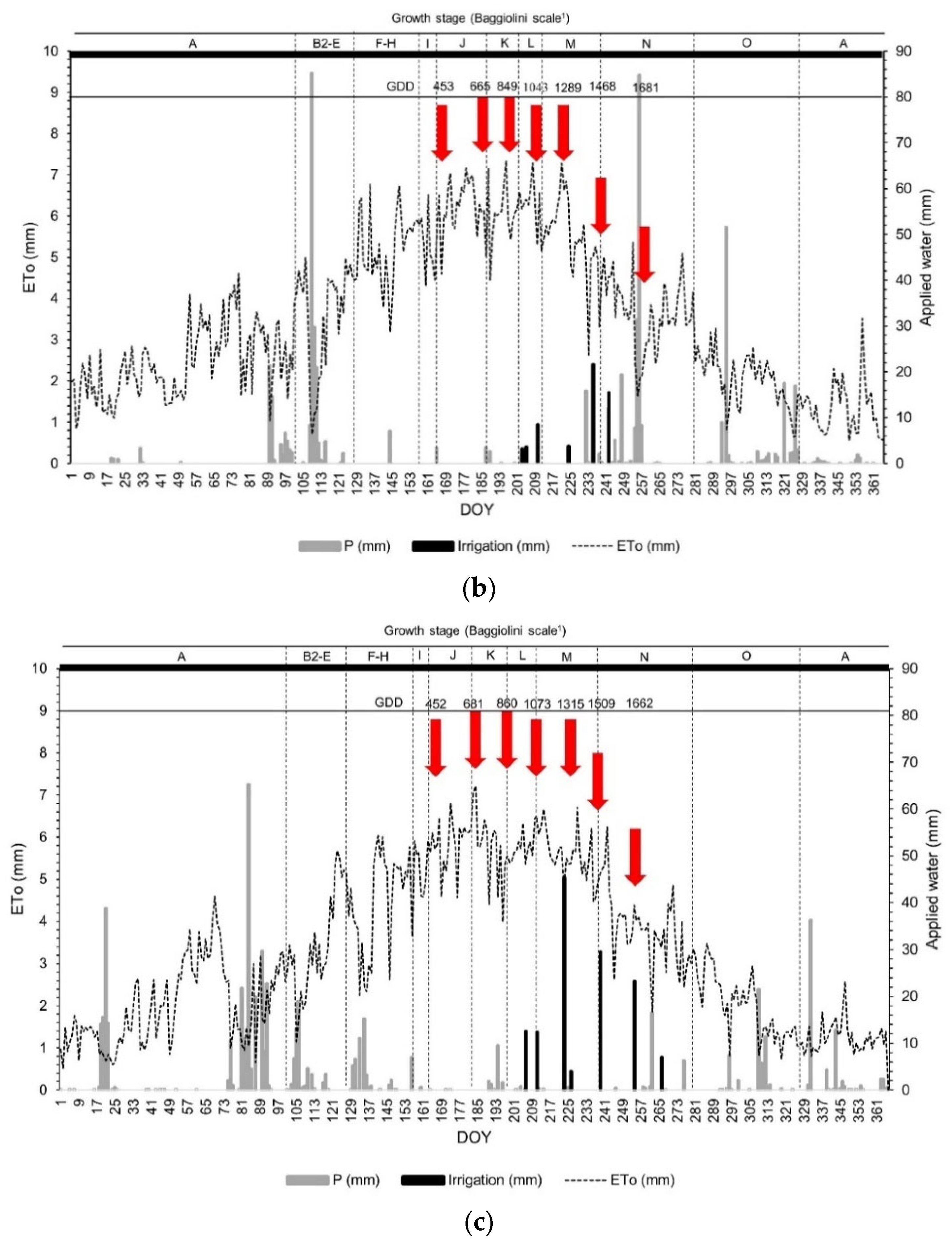
3.1. Analysis of the Water Stress Integral (Sψ)

Analysing the evolution of the grapevine water status throughout the growth cycle in different years, the computed Sψ followed the same trend in 2018 and 2020 (Figure 5). In 2019, the increase in Sψ between the last two measurements decreased due to the effect of more than 130 mm of rainfall four days before the last measurement (Figure 3b). Sψ showed no differences between treatments until the last days of July (closed cluster). Afterwards, water stress differences were visible. The Sψ experienced by the rain-fed (T1) and irrigation (T2) treatments differed significantly. The vines of the other treatments showed intermediate values between those from the irrigation and the more intense stress treatment (rain-fed), although in 2020, salt treatments were closer to the irrigation regime with good quality water, possibly due to the additional effect of recorded rainfall. Sψ values equal to 64.3 MPa×days (T1) and 35.3 MPa×days (T2) were reached in the last sampling date of 2018 (19 September). Such values were equal to 47.6 MPa×days (T1) and 24 MPa×days (T2) in the last sampling date of 2019 (18 September). Similar values were obtained for the same treatments in the last sampling date of 2020 (10 September) with 46 MPa×days and 30 MPa×days. Although the pattern of Sψ was similar in 2018 and 2020 (both years had a similar rainfall in the growth cycle), the Sψ values of rain-fed (T1) and irrigation (T2) treatments were higher in 2018, especially in T1. Although rainfall events were recorded between the last two measurements in 2018 (35 mm), the GDD accumulated in that period (326) more than doubled that accumulated in 2020 (153) (Figure 5). The evaporative demand between the last two measurements was also higher in 2018 (102 mm) than in 2020 (69 mm). In 2020, the high and well-distributed rainfall recorded in the first months of 2020 (especially in January, March, and April) probably replenished soil water reserves (Figure 3c). The cumulative rainfall in the first months of 2020 (from January to April) was 345 mm (more than 60% of annual rainfall), 132% higher than the cumulative rainfall in the first four months of 2018, and 57% higher than the cumulative rainfall in the same period in 2019. On the other hand, evaporative demand in that period time was 258 mm, 7% lower than the evaporative demand in the first four months of 2018, and 16% lower than the evaporative demand in the same period in 2019. As a result, the water available in the soil profile reserve at the beginning of the grapevine activity was higher, and the water needs of the grapevine could be supplied for a longer period of time. Therefore, this resulted in a water status of the grapevine with lower Sψ values at the last sampling date, similar to that obtained at the last sampling date of 2019 when 132 mm of rainfall were previously recorded. After that rain event, the water status of the vine clearly decreased, and this was reflected in the Ψstem as a punctual measure from −1.28 MPa (at the end of August) to −0.58 MPa (at the last measurement in September). It was also reflected in Sψ with a decreasing slope of the line joining the two final measurements (Figure 5). These were the reasons why Sψ at the last sampling date of 2020, when the rainfall recorded during the growth cycle was very low (compared to 2019), was similar to Sψ at the last sampling date of 2019. The mentioned weather conditions determined the grapevine water status and the greatest accumulated water stress at the end of the 2018 growth cycle.

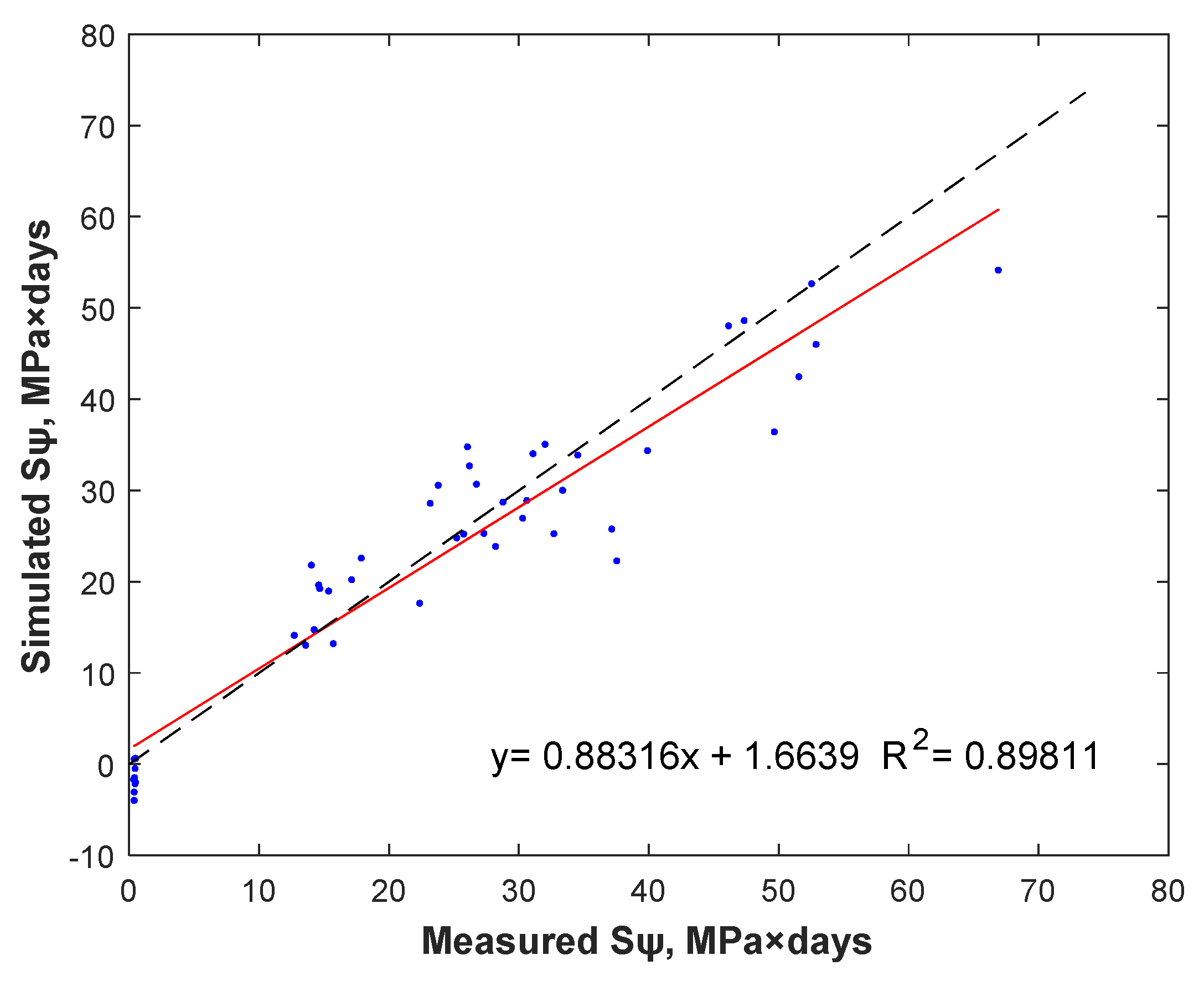
3.2. Estimating Sψ Based on ANN Models with RGB Data

The application of ANN based on the combination of normalised RGB bands and GCC provided better results than those obtained from MRM with the same predicted variables. Table 4 shows the validation results for estimating Sψ in each studied season and every combination of years using ANN and MRM. The ANN model with the best performance was the one that employed 2018 data with R2 = 0.98, RMSE = 1.91 MPa×days, and RE = 10.84% (statistical parameters in bold). For that same season, results obtained from MRM were worse, with lower R2 (0.65) and RE four times higher (48%). Analysing the ANN validation results obtained in 2019, the model showed an RE too high (50.44%). The results obtained in 2020 were better than those obtained in 2019, although the RE was still too high to estimate Sψ. Analysing the seasons’ data in pairs or together, the ANN model that used 2018 and 2020 data presented the best performance (R2 = 0.83, RMSE = 4.9 MPa×days, and RE = 33.47%), even though the RE was high for a predictive model. The best results obtained integrating 2018 and 2020 could be due to similar water status development in both years. Regarding MRM, R2 values were lower than those obtained from ANN models in all seasons, with higher errors.
Figure 6 shows the correlation between the measured and predicted Sψ in the validation process of the RGB ANN model, with the best performance in the 2018 season. The model tends to slightly underestimate Sψ.

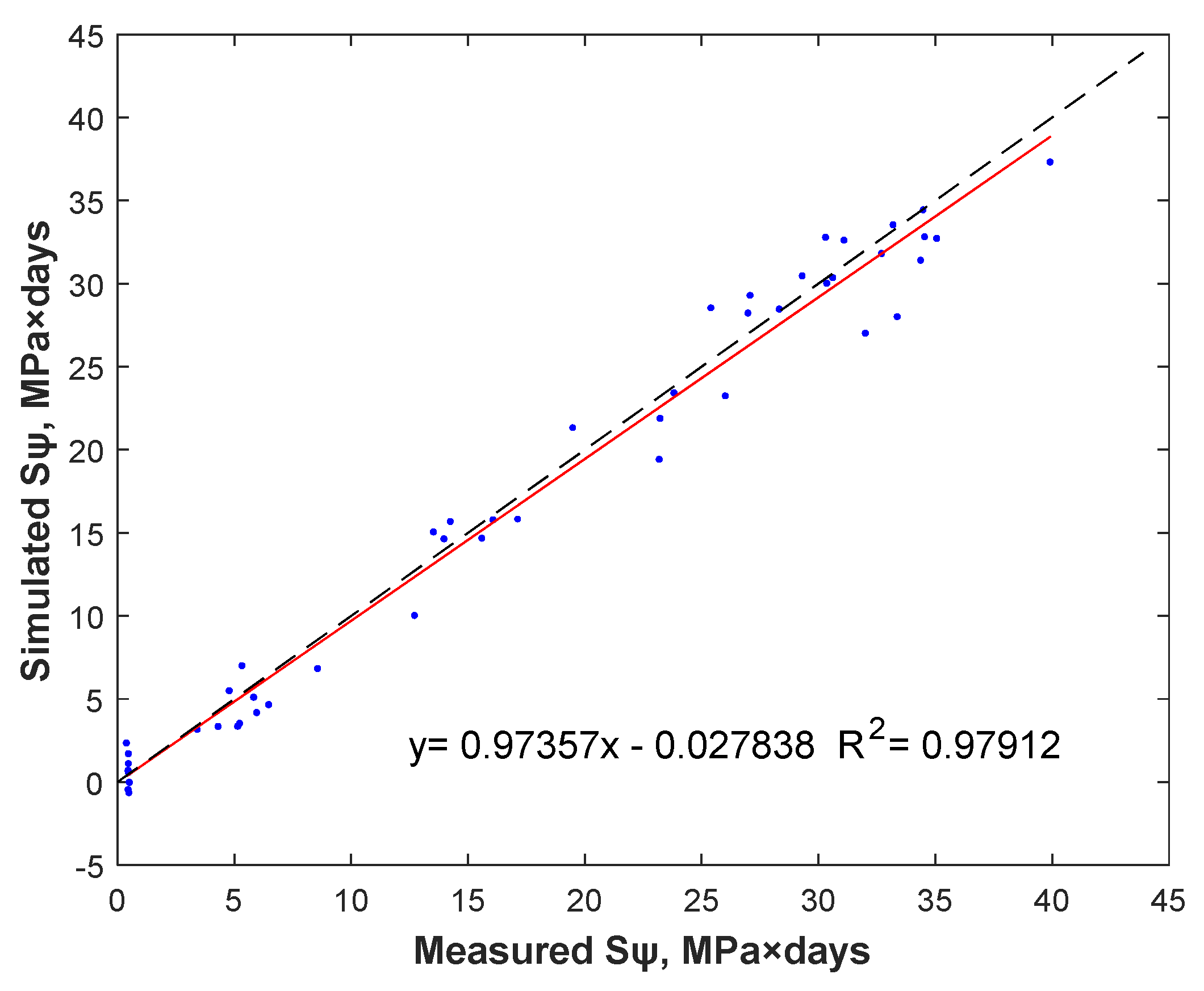
3.3. Estimating Sψ Based on ANN Models with Multispectral Data

ANN models based on the combination of multispectral sensor bands and GCCMULTI provided better results than those obtained from MRM in all analysed years and combined seasons (Table 5). The model with the best performance using ANN was that obtained with 2018 data with R2 = 0.9 and RE = 22.97% (statistical parameters in bold). To analyse the interannual effects, ANN models were evaluated for years in pairs, and as all years together. The best model combining two seasons was that obtained from the 2018 and 2020 data, with the highest R2 (0.87) and the lowest RE (33.73%). In the models generated with RGB data and those generated with multispectral data, the statistical parameters were worse when 2019 data were used. This trend was more accentuated when RGB data were used, showing higher stability when employing multispectral data. Moreover, except for 2018, the ANN models with multispectral data provided the best statistical parameters, with higher R2 and lower RE. In addition, multispectral MRM also provided better statistics than RGB MRM, with slightly higher R2 and lower RE in most of the seasons analysed. However, they were not better than the statistics obtained with multispectral ANN in any analysis.
The correlation between the measured and predicted Sψ in the validation process of the multispectral ANN model, with the best performance in the 2018 season, is shown in Figure 7. In general, values of Sψ between 10 and 30 MPa×days were mostly overestimated, while Sψ values above 30 MPa×days were largely underestimated.

4. Discussion

In agriculture, ANN models are the most popular ML tools used in crop management, water management, and soil management approaches [29]. Moreover, ANN is a widely utilized ML technique for crop water stress determination [10]. Several studies have employed ANN models in order to use aerial spectral information to predict crop water stress, as in this study. Romero et al. [23] obtained aerial multispectral imagery to calculate various VIs which were applied as inputs to one of two ANN models for estimating Ψstem. Their model showed a strong correlation between the simulated Ψstem and the measured Ψstem, with an R2 value of 0.53 for the validation data. In our study, when RGB, multispectral bands, and GCC (which is representative of canopy vigour) were used as inputs for ANN models, the R2 values of all the models generated were higher than 0.53 in all years, with a maximum value of 0.98 and a minimum of 0.64. Poblete et al. [22] used ANN models to predict the spatial variability in Ψstem in vineyards. They used multispectral imagery and used separate bands as inputs to the ANN models. Good results were obtained in the comparisons of the simulated Ψstem versus the measured Ψstem, with R2 and RE values from 0.56 to 0.87 and from 9.11 to 16.50%, respectively. In the present study, the R2 values obtained were slightly better than (considering all growing seasons), or in some cases similar to, the R2 values obtained in the work of Poblete et al. [22]. The RE values in our study were higher than those obtained in their study, with the sole exception of the model obtained for 2018 RGB data with RE = 10.84%.
The results derived from this research proved that the ANN models provided better statistics than those derived from MRM models. Analysing ANN models, multispectral information showed slightly more stable results when analysing interannual effects than RGB-based information with RE between 23 and 44%, while the maximum error reached with RGB ANN models was 50%. Moreover, except for 2018, when the best performing model was that for RGB, the R2 is higher and the RE is either the same or lower in the multispectral sensor-based models as compared with the RGB-based models for all the other years and combinations of years. Nevertheless, although the results obtained with spectral information based on the visible domain have not been the best, they were not excessively different from those obtained with multispectral information, and are of interest for the development of predictive models of biophysical and biochemical parameters of crops, such as water stress. However, few authors have used visible bands to predict water status [46,47,48,49]. Rapaport et al. [50] correlated hyperspectral signatures to midday leaf water potential using the partial least squares regression technique, obtaining R2 (0.88) and error (9%) values. Midday leaf water potential was better explained by combining the reflectance decrease at 530–550 nm with the opposed increased around 1500 nm. The reflectance decrease at 550 nm (green band of visible electromagnetic spectrum) is mainly associated with adjustments of photosynthetic and photoprotective pigments, such as anthocyanin [51]; moreover, the reflectance increase around 1500 nm is strongly affiliated with a direct decrease in leaf water content [52]. Moreover, the adequate performance of these variables could be due to the higher spatial resolution of the RGB data. High spatial resolution compensates the lower reflectance in the visible region of the green band compared with that in the infrared and red-edge bands [53], and could also compensate the poor radiometric quality of these types of cameras. Additionally, this high resolution leads to more precise GCC values. According to the results, using high-resolution RGB products (GSD = 2 cm) to predict Sψ instead of traditional multispectral products would have several advantages, such as cost reduction (RGB sensors are much less expensive than multispectral sensors); more straightforward data processing; less sun glint and fewer hotspot effects, which are typical of multispectral images [54]; and a greater possibility of obtaining the geometric characteristics of the plants due to the high spatial resolution of the generated products. Therefore, using only RGB products as inputs to ANN models can offer a good solution for measuring accumulated water stress.
Unlike most of the works found in the bibliography that estimated water status using punctual measures such as stem or leaf water potential, in our study the Sψ was used. This variable enabled the analysis of the effect of the cumulative water deficit duration and intensity throughout the growing season considering midday Ψstem measurements over a chosen period of time [35], coinciding with the fact that the accumulated effects of water stress are shown in plant tissues affecting the spectral response of leaves [15,55]. Some studies have employed this parameter, as an index of water stress, and it was correlated with volume growth, pre-dawn xylem water potential, soil volumetric water content [11], productivity [56], and mortality [57]. It also has been widely used for irrigation management and modelling in agricultural crops [58,59].
Despite the good performance of ANN regression models in predicting Sψ, especially in the 2018 season, the models did not follow the same Sψ prediction trends in the other years, in which R2 values decreased and RE values increased. This is particularly relevant when data from more than one season were combined together, suggesting that a unique robust estimation of plant water status valid for more than a single season might be difficult to implement at a commercial level. Differences in canopy management, crop loads, and the seasonal development of water stress might influence the relationship between remote sensing and on-the-ground estimations of water status. In this sense, the continued application over more than a season of different irrigation regimes might have affected canopy morphology and growth, indeed making noise in the water status estimation from the RGB bands.
As a consequence, the implementation of the here proposed methodology did not allow us to generate a general predictive model of water status for the three analysed seasons due to the differentiated interannual response of the crop on biotic and abiotic factors. Field punctual measurements in each growing season are required to estimate water status because vine water status depends on the availability of water (soil water, rainfall, and irrigation), weather conditions (temperature, ET0, relative humidity, etc.) and leaf area, as well as the ability of the vine to absorb and transport water to its organs [60]. Among environmental factors, the climate has a more significant impact on vine development. Moreover, climatic conditions vary from one year to the other and are difficult to control [61]. Buesa et al. [59] also found that the seasonal variation in water status was also affected by the soil water available at the beginning of the stress period and the weather conditions during the growth cycle, determining the exact timing of water stress and its intensity difference between years. More effort is therefore needed to integrate additional vines and environmental variables into the generated models to improve the water status estimations.

5. Conclusions

The use of machine learning methods such as ANN models are a powerful tool for processing remote sensing data obtained from UAVs to develop models for estimating Sψ in the same seasons in which field measurements were recorded, as the fits of these models were better than those obtained from linear regression models. Good results were obtained using RGB bands and the GCC as the inputs for the ANN models. Although the results obtained were more stable in the different years with multispectral sensors, the use of conventional RGB cameras is a promising alternative due to its lower cost compared with multispectral and thermal sensors, and the easier photogrammetric processing of the images. High-resolution RGB images permit the precise segmentation of vegetation image data, which is essential for avoiding soil effects and obtaining accurate GCC values.
Interannual differences in the crop response to biotic and abiotic factors did not make it possible to generate a general model that estimates the water stress in vineyard. Thus, it is still necessary to perform punctual measurements of stem water potential in some plants to generate specific models that could be applied to the whole extent of the vineyard. The methodology of this research is a first step for the development of future predictive models of water status. It could be integrated in a farmer decision support system, since from a few measurements of water potential in the field and the spectral information derived from a UAV, the farmer will be able to know the water status of the entire vineyard plot, thus making irrigation programming more efficient. Therefore, future studies will attempt to predict the water status on a specific date in any year using a previously developed generalizable calibrated model by extending the number of seasons analysed. This study was carried out in a cv. Monastrell vineyard; future efforts will attempt to demonstrate that the calibrated model can be applied to vineyards of different varieties in any location.

Author Contributions

P.L.-G. is the main author of this paper together with R.B. who is the corresponding author. P.L.-G., A.M.-M. and E.P.P.-Á. performed the field data collection and M.A.M. executed UAV flights. J.F.O., M.A.M., R.B. and D.I. performed financial and contractual duties. All authors have read and agreed to the published version of the manuscript.

Funding

This research was funded by the Ministry of Science, Innovation and Universities, grant numbers PID2020-115998RB-C22, AGL2017-83738-C3-3-R, and RTC-2017-6365-2; by the Government of Castilla-La Mancha, grant number SBPLY/17/180501/000251; by FEDER funds, grant number AEI-FEDER Project AGL2017-83738-C3-3-R; and by EU HORIZON-CL6-2021 GOVERNANCE-01 CALL Project CHAMELEON 101060529.

Institutional Review Board Statement

Not applicable.

Informed Consent Statement

Not applicable.

Data Availability Statement

Not applicable.

Acknowledgments

The authors would like to thank the University Teaching Scholarship (Formación de Profesorado Universitario, FPU) for financial support. The authors also wish to thank the commercial vineyard owner; the Water User Association “Las Colleras”, located in Fuente-Álamo, Albacete, Spain; and the field technicians for their work and involvement in the trial.

Conflicts of Interest

The authors declare no conflict of interest.

References

  1. OIV Data Base. Available online: http://www.oiv.int/es/statistiques/recherche (accessed on 24 February 2022).
  2. ESYRCE. Available online: https://www.mapa.gob.es/es/estadistica/temas/estadisticas-agrarias/totalespanayccaa2020_tcm30-553610.pdf (accessed on 22 April 2021).
  3. Mirás-Avalos, J.M.; Intrigliolo, D.S. Grape Composition under Abiotic Constrains: Water Stress and Salinity. Front. Plant Sci. 2017, 8, 851. [Google Scholar] [CrossRef]
  4. Hunink, J.; Simons, G.; Suárez-Almiñana, S.; Solera, A.; Andreu, J.; Giuliani, M.; Zamberletti, P.; Grillakis, M.; Koutroulis, A.; Tsanis, I.; et al. A Simplified Water Accounting Procedure to Assess Climate Change Impact on Water Resources for Agriculture across Different European River Basins. Water 2019, 11, 1976. [Google Scholar] [CrossRef]
  5. Antunes, P.; Santos, R.; Cosme, I.; Osann, A.; Calera, A.; De Ketelaere, D.; Spiteri, A.; Mejuto, M.F.; Andreu, J.; Momblanch, A.; et al. A Holistic Framework to Assess the Sustainability of Irrigated Agricultural Systems. Cogent Food Agric. 2017, 3, 1323542. [Google Scholar] [CrossRef]
  6. Romero, P.; Fernández-Fernández, J.I.; Martinez-Cutillas, A. Physiological Thresholds for Efficient Regulated Deficit-Irrigation Management in Winegrapes Grown under Semiarid Conditions. Am. J. Enol. Vitic. 2010, 61, 300–312. [Google Scholar]
  7. Miras-Avalos, J.M.; Araujo, E.S. Optimization of Vineyard Water Management: Challenges, Strategies, and Perspectives. Water 2021, 13, 746. [Google Scholar] [CrossRef]
  8. Choné, X.; VanLeeuwen, C.; Dubourdieu, D.; Gaudillère, J.P. Stem Water Potential Is a Sensitive Indicator of Grapevine Water Status. Ann. Bot. 2001, 87, 477–483. [Google Scholar] [CrossRef]
  9. Acevedo-Opazo, C.; Ortega-Farias, S.; Fuentes, S. Effects of Grapevine (Vitis Vinifera L.) Water Status on Water Consumption, Vegetative Growth and Grape Quality: An Irrigation Scheduling Application to Achieve Regulated Deficit Irrigation. Agric. Water Manag. 2010, 97, 956–964. [Google Scholar] [CrossRef]
  10. Virnodkar, S.S.; Pachghare, V.K.; Patil, V.C.; Jha, S.K. Remote Sensing and Machine Learning for Crop Water Stress Determination in Various Crops: A Critical Review. Precision Agric. 2020, 21, 1121–1155. [Google Scholar] [CrossRef]
  11. Gonzalez-Benecke, C.A.; Dinger, E.J. Use of Water Stress Integral to Evaluate Relationships between Soil Moisture, Plant Water Stress and Stand Productivity in Young Douglas-Fir Trees. New For. 2018, 49, 775–789. [Google Scholar] [CrossRef]
  12. Suárez, L.; Zarco-Tejada, P.J.; González-Dugo, V.; Berni, J.A.J.; Sagardoy, R.; Morales, F.; Fereres, E. Detecting Water Stress Effects on Fruit Quality in Orchards with Time-Series PRI Airborne Imagery. Remote Sens. Environ. 2010, 114, 286–298. [Google Scholar] [CrossRef]
  13. Srinivasan, A. Handbook of Precision Agriculture: Principles and Applications; Food Products Press: Binghamton, NY, USA, 2006; ISBN 9781482277968. [Google Scholar]
  14. Santesteban, L.G. Precision Viticulture and Advanced Analytics. A Short Review. Food Chem. 2019, 279, 58–62. [Google Scholar] [CrossRef]
  15. Cogato, A.; Yassir, S.; Jewan, Y.; Wu, L.; Marinello, F.; Meggio, F.; Sivilotti, P.; Sozzi, M.; Pagay, V. Drought Stress Impacts on Grapevines ( Vitis Vinifera L.) under High VPD Conditions: Physiological and Spectral Responses. Agronomy 2022, 12, 1819. [Google Scholar] [CrossRef]
  16. López-García, P.; Intrigliolo, D.S.; Moreno, M.A.; Martínez-Moreno, A.; Ortega, J.F.; Pérez-Álvarez, E.P.; Ballesteros, R. Assessment of Vineyard Water Status by Multispectral and RGB Imagery Obtained from an Unmanned Aerial Vehicle. Am. J. Enol. Vitic. 2021, 72, 285–297. [Google Scholar] [CrossRef]
  17. Zarco-Tejada, P.J.; Berjón, A.; López-Lozano, R.; Miller, J.R.; Martín, P.; Cachorro, V.; González, M.R.; de Frutos, A. Assessing Vineyard Condition with Hyperspectral Indices: Leaf and Canopy Reflectance Simulation in a Row-Structured Discontinuous Canopy. Remote Sens. Environ. 2005, 99, 271–287. [Google Scholar] [CrossRef]
  18. Berni, J.; Zarco-Tejada, P.J.; Suárez, L.; Fereres, E. Thermal and Narrowband Multispectral Remote Sensing for Vegetation Monitoring from an Unmanned Aerial Vehicle. IEEE Trans. Geosci. Remote Sens. 2009, 47, 722–738. [Google Scholar] [CrossRef]
  19. Baluja, J.; Diago, M.P.; Balda, P.; Zorer, R.; Meggio, F.; Morales, F.; Tardaguila, J. Assessment of Vineyard Water Status Variability by Thermal and Multispectral Imagery Using an Unmanned Aerial Vehicle (UAV). Irrig. Sci. 2012, 30, 511–522. [Google Scholar] [CrossRef]
  20. Ballesteros, R.; Ortega, J.F.; Hernández, D.; Moreno, M.Á. Characterization of Vitis Vinifera L. Canopy Using Unmanned Aerial Vehicle-Based Remote Sensing and Photogrammetry Techniques. Am. J. Enol. Vitic. 2015, 66, 120–129. [Google Scholar] [CrossRef]
  21. Ballesteros, R.; Ortega, J.F.; Hernandez, D.; Moreno, M.A. Onion Biomass Monitoring Using UAV-Based RGB Imaging. Precis. Agric. 2018, 19, 840–857. [Google Scholar] [CrossRef]
  22. Poblete, T.; Ortega-Farías, S.; Moreno, M.A.; Bardeen, M. Artificial Neural Network to Predict Vine Water Status Spatial Variability Using Multispectral Information Obtained from an Unmanned Aerial Vehicle (UAV). Sensors 2017, 17, 2488. [Google Scholar] [CrossRef]
  23. Romero, M.; Luo, Y.; Su, B.; Fuentes, S. Vineyard Water Status Estimation Using Multispectral Imagery from an UAV Platform and Machine Learning Algorithms for Irrigation Scheduling Management. Comput. Electron. Agric. 2018, 147, 109–117. [Google Scholar] [CrossRef]
  24. Bishop, C.M. Pattern Recognition and Machine Learning; Springer: New York, NY, USA, 2006. [Google Scholar]
  25. Chlingaryan, A.; Sukkarieh, S.; Whelan, B. Machine Learning Approaches for Crop Yield Prediction and Nitrogen Status Estimation in Precision Agriculture: A Review. Comput. Electron. Agric. 2018, 151, 61–69. [Google Scholar] [CrossRef]
  26. Pôças, I.; Gonçalves, J.; Costa, P.M.; Gonçalves, I.; Pereira, L.S.; Cunha, M. Hyperspectral-Based Predictive Modelling of Grapevine Water Status in the Portuguese Douro Wine Region. Int. J. Appl. Earth Obs. Geoinf. 2017, 58, 177–190. [Google Scholar] [CrossRef]
  27. Moshou, D.; Pantazi, X.E.; Kateris, D.; Gravalos, I. Water Stress Detection Based on Optical Multisensor Fusion with a Least Squares Support Vector Machine Classifier. Biosyst. Eng. 2014, 117, 15–22. [Google Scholar] [CrossRef]
  28. Loggenberg, K.; Strever, A.; Greyling, B.; Poona, N. Modelling Water Stress in a Shiraz Vineyard Using Hyperspectral Imaging and Machine Learning. Remote Sens. 2018, 10, 202. [Google Scholar] [CrossRef]
  29. Liakos, K.G.; Busato, P.; Moshou, D.; Pearson, S.; Bochtis, D. Machine Learning in Agriculture: A Review. Sensors 2018, 18, 2674. [Google Scholar] [CrossRef] [PubMed]
  30. Krishna, G.; Sahoo, R.N.; Singh, P.; Bajpai, V.; Patra, H.; Kumar, S.; Dandapani, R.; Gupta, V.K.; Viswanathan, C.; Ahmad, T.; et al. Comparison of Various Modelling Approaches for Water Deficit Stress Monitoring in Rice Crop through Hyperspectral Remote Sensing. Agric. Water Manag. 2019, 213, 231–244. [Google Scholar] [CrossRef]
  31. Climate Zones. National Geographic Institute (NGI). Available online: https://www.ign.es/espmap/mapas_clima_bach/pdf/Clima_Mapa_1_2texto.pdf (accessed on 9 February 2022).
  32. Amerine, M.A.; Winkler, A.J. Composition and Quality of Musts and Wines of California Grapes. Hilgardia. A J. Agric. Sci. Publ. Calif. Agric. Exp. Stn. 1944, 15, 184. [Google Scholar] [CrossRef]
  33. Baggiolini, M. Les Stades Repères Dans Le Développment Annuel de La Vigne et Leur Utilisation Pratique. Rev. Rom. D’agric. D’arboric. 1952, 8, 4–6. [Google Scholar]
  34. Martínez-Moreno, A.; Pérez-Álvarez, E.P.; López-Urrea, R.; Paladines-Quezada, D.F.; Moreno-Olivares, J.D.; Intrigliolo, D.S.; Gil-Muñoz, R. Effects of Deficit Irrigation with Saline Water on Wine Color and Polyphenolic Composition of Vitis Vinifera L. Cv. Monastrell. Sci. Hortic. 2021, 283, 110085. [Google Scholar] [CrossRef]
  35. Myers, B.J. Water Stress Integral, a Link between Short-Term Stress and Long-Term Growth. Tree Physiol. 1988, 4, 315–323. [Google Scholar] [CrossRef]
  36. Hernandez-lopez, D.; Felipe-garcia, B.; Gonzalez-aguilera, D.; Arias-perez, B. An Automatic Approach to UAV Flight Planning and Control for Photogrammetric Applications: A Test Case in the Asturias Region (Spain). Photogramm. Eng. Remote Sens. 2013, 79, 87–98. [Google Scholar] [CrossRef]
  37. Woebbecke, D.M.; Meyer, G.E.; Von Bargen, K.; Mortensen, D.A. Color Indices for Weed Identification under Various Soil, Residue, and Lighting Conditions. Trans. Am. Soc. Agric. Eng. 1995, 38, 259–269. [Google Scholar] [CrossRef]
  38. Ribeiro-Gomes, K.; Hernandez-Lopez, D.; Ballesteros, R.; Moreno, M.A. Approximate Georeferencing and Automatic Blurred Image Detection to Reduce the Costs of UAV Use in Environmental and Agricultural Applications. Biosyst. Eng. 2016, 151, 308–327. [Google Scholar] [CrossRef]
  39. Córcoles, J.I.; Ortega, J.F.; Hernández, D.; Moreno, M.A. Estimation of Leaf Area Index in Onion (Allium Cepa L.) Using an Unmanned Aerial Vehicle. Biosyst. Eng. 2013, 115, 31–42. [Google Scholar] [CrossRef]
  40. Steduto, P.; Hsiao, T.C.; Raes, D.; Fereres, E. AquaCrop—The FAO Crop Model to Simulate Yield Response to Water: I. Concepts and Underlying Principles. Agron. J. 2009, 101, 426. [Google Scholar] [CrossRef]
  41. Agatonovic-Kustrin, S.; Beresford, R. Basic Concepts of Artificial Neural Network (ANN) Modeling and Its Application in Pharmaceutical Research. J. Pharm. Biomed. Anal. 2000, 22, 717–727. [Google Scholar] [CrossRef]
  42. Kumar, M.; Raghuwanshi, N.S.; Singh, R.; Wallender, W.W.; Pruitt, W.O. Estimating Evapotranspiration Using Artificial Neural Network. J. Irrig. Drain. Eng. 2002, 128, 224–233. [Google Scholar] [CrossRef]
  43. Kubat, M. An Introduction to Machine Learning, 2nd ed.; Springer: Cham, Switzerland, 2017; ISBN 9783319639130. [Google Scholar]
  44. Bishop, C.M. Neural Networks for Pattern Recognition; Clarendon Press: Oxford, UK, 1995; ISBN 9780198538646. [Google Scholar]
  45. Ballesteros, R.; Ortega, J.F.; Moreno, M.Á. FORETo: New Software for Reference Evapotranspiration Forecasting. J. Arid Environ. 2016, 124, 128–141. [Google Scholar] [CrossRef]
  46. Pôças, I.; Rodrigues, A.; Gonçalves, S.; Costa, P.M.; Gonçalves, I.; Pereira, L.S.; Cunha, M. Predicting Grapevine Water Status Based on Hyperspectral Reflectance Vegetation Indices. Remote Sens. 2015, 7, 16460–16479. [Google Scholar] [CrossRef]
  47. Rodríguez-Pérez, J.R.; Riaño, D.; Carlisle, E.; Ustin, S.; Smart, D.R. Evaluation of Hyperspectral Reflectance Indexes to Detect Grapevine Water Status in Vineyards. Am. J. Enol. Vitic. 2007, 58, 302–317. [Google Scholar]
  48. Rossini, M.; Fava, F.; Cogliati, S.; Meroni, M.; Marchesi, A.; Panigada, C.; Giardino, C.; Busetto, L.; Migliavacca, M.; Amaducci, S.; et al. Assessing Canopy PRI from Airborne Imagery to Map Water Stress in Maize. ISPRS J. Photogramm. Remote Sens. 2013, 86, 168–177. [Google Scholar] [CrossRef]
  49. Zarco-Tejada, P.J.; González-Dugo, V.; Williams, L.E.; Suárez, L.; Berni, J.A.J.; Goldhamer, D.; Fereres, E. A PRI-Based Water Stress Index Combining Structural and Chlorophyll Effects: Assessment Using Diurnal Narrow-Band Airborne Imagery and the CWSI Thermal Index. Remote Sens. Environ. 2013, 138, 38–50. [Google Scholar] [CrossRef]
  50. Rapaport, T.; Hochberg, U.; Shoshany, M.; Karnieli, A.; Rachmilevitch, S. Combining Leaf Physiology, Hyperspectral Imaging and Partial Least Squares-Regression (PLS-R) for Grapevine Water Status Assessment. ISPRS J. Photogramm. Remote Sens. 2015, 109, 88–97. [Google Scholar] [CrossRef]
  51. Viña, A.; Gitelson, A.A. Sensitivity to Foliar Anthocyanin Content of Vegetation Indices Using Green Reflectance. IEEE Geosci. Remote Sens. Lett. 2011, 8, 464–468. [Google Scholar] [CrossRef]
  52. Eitel, J.U.H.; Gessler, P.E.; Smith, A.M.S.; Robberecht, R. Suitability of Existing and Novel Spectral Indices to Remotely Detect Water Stress in Populus Spp. For. Ecol. Manag. 2006, 229, 170–182. [Google Scholar] [CrossRef]
  53. Carter, G.A. Primary and Secondary Effects on Water Content on the Spectral Reflectance of Leaves. Am. J. Bot. 1991, 78, 916–924. [Google Scholar] [CrossRef]
  54. Ortega-Terol, D.; Hernandez-Lopez, D.; Ballesteros, R.; Gonzalez-Aguilera, D. Automatic Hotspot and Sun Glint Detection in UAV Multispectral Images. Sensors 2017, 17, 2352. [Google Scholar] [CrossRef]
  55. Marín-Ortiz, J.C.; Gutierrez-Toro, N.; Botero-Fernández, V.; Hoyos-Carvajal, L.M. Linking Physiological Parameters with Visible/near-Infrared Leaf Reflectance in the Incubation Period of Vascular Wilt Disease. Saudi J. Biol. Sci. 2020, 27, 88–99. [Google Scholar] [CrossRef]
  56. De la Rosa, J.M.; Conesa, M.R.; Domingo, R.; Aguayo, E.; Falagán, N.; Pérez-Pastor, A. Combined Effects of Deficit Irrigation and Crop Level on Early Nectarine Trees. Agric. Water Manag. 2016, 170, 120–132. [Google Scholar] [CrossRef]
  57. Hanson, P.J.; Todd, J.; Amthor, J.S. Erratum: A Six-Year Study of Sapling and Large-Tree Growth and Mortality Responses to Natural and Induced Variability in Precipitation and Throughfall (Tree Physiology 21 (345–358)). Tree Physiol. 2001, 21, 1158. [Google Scholar] [CrossRef]
  58. Ballester, C.; Castel, J.; Intrigliolo, D.S.; Castel, J.R. Response of Navel Lane Late Citrus Trees to Regulated Deficit Irrigation: Yield Components and Fruit Composition. Irrig. Sci. 2013, 31, 333–341. [Google Scholar] [CrossRef]
  59. Buesa, I.; Pérez, D.; Castel, J.; Intrigliolo, D.S.; Castel, J.R. Effect of Deficit Irrigation on Vine Performance and Grape Composition of Vitis Vinifera L. Cv. Muscat of Alexandria. Aust. J. Grape Wine Res. 2017, 23, 251–259. [Google Scholar] [CrossRef]
  60. Baeza, P.; Junquera, P.; Peiro, E.; Lissarrague, J.R.; Uriarte, D.; Vilanova, M. Effects of Vine Water Status on Yield Components, Vegetative Response and Must and Wine Composition. Adv. Grape Wine Biotechnol. 2019. [Google Scholar] [CrossRef] [Green Version]
  61. Van Leeuwen, C.; Darriet, P. The Impact of Climate Change on Viticulture and Wine Quality. J. Wine Econ. 2016, 11, 150–167. [Google Scholar] [CrossRef] [Green Version]
Figure 1. Flowchart of the methodology of this study carried out in a vineyard cv. Monastrell, located in south-eastern Spain.
Agronomy 12 02122 g001
Figure 2. Location of the commercial vineyard in south-eastern Spain, and the distribution of experimental units in 2018, 2019, and 2020. In the lefthand image, the white dashed line outlines the blocks of the experiment (four blocks). In the righthand image, each symbol corresponds to a grapevine plant.
Agronomy 12 02122 g002
Figure 3. Rainfall (P), irrigation, reference evapotranspiration (ET0), and growing degree days (GDD) during the days of the year (DOY) of the growing cycle in a vineyard located in Fuente-Álamo, Spain, in (a) 2018; (b) 2019; and (c) 2020. The red arrow represents the date of imagery acquisition and Ψstem measurement. 1 Baggiolini scale: [33] (A: winter dormancy, B: bleeding, B2: bud swelling, C: bud burst, D: green shoot, E: 2 to 3 leaves unfolded, F: inflorescence clearly visible, G: separate inflorescences, H: separate floral button, I: flowering, J: fruit set, K: pea-sized berry, L: closed bunch, M: veraison, N: berry ripening, O: leaf fall).
Agronomy 12 02122 g003aAgronomy 12 02122 g003b
Figure 4. Flowchart of the segmentation of vegetation by LAIC software in a vineyard located in Fuente-Álamo, Spain.
Agronomy 12 02122 g004
Figure 5. Water stress integral (Sψ; MPa×days) of studied vineyard located in Fuente-Álamo, Spain, for different experimental treatments during the 2018, 2019, and 2020 seasons. GDD: growing degree days of measurement and flight dates in each year.
Agronomy 12 02122 g005
Figure 6. Correlation between the measured and predicted Sψ using the best predictive RGB ANN model in the 2018 season.
Agronomy 12 02122 g006
Figure 7. Correlation between the measured and predicted Sψ using the best predictive multispectral ANN model in the 2018 season.
Agronomy 12 02122 g007
Table 1. Annual and growing season (from April to the end of September) rainfall and reference evapotranspiration (ET0) values from the studied vineyard cv. Monastrell located in south-eastern Spain.
Rainfall (mm)ET0 (mm)
2018
Annual4061171
Growing season230834
2019
Annual5501270
Growing season400879
2020
Annual5531185
Growing season166853
Table 2. Description of the experimental treatments carried out in a vineyard cv. Monastrell, located in south-eastern Spain, in the 2018, 2019, and 2020 seasons.
TreatmentDescription
T1Rain-fed
T2Irrigation with standard-quality water
T3Irrigation with added sulphates (Na2SO4 and MgSO4)
T4Irrigation with added NaCl
T5Irrigation with added sulphates starting at veraison
T6Irrigation with added NaCl starting at veraison
Table 3. Characteristics of the sensors mounted on the UAV flown in a vineyard cv. Monastrell, located in south-eastern Spain, in the 2018, 2019, and 2020 seasons.
Parrot SEQUOIASony ILCE-5100
Sensor4.8 mm × 3.6 mm CCD 123.5 mm × 15.6 mm CMOS 2
Pixel size (μm)3.75 × 3.754 × 4
Image resolution (columns and rows of pixels)1280 × 9606000 × 4000
Focal length (mm)3.9820
Spectral bandsGreen: 530–570 nm
Red: 640–680 nm
Red-edge: 730–740 nm
Near-infrared: 770–810 nm
Red
Green
Blue
1 CCD: charge-coupled device; 2 CMOS: complementary metal oxide semiconductor.
Table 4. Validation results (R2: determination coefficient, RMSE: root mean squared error, and RE: relative error) for the ANN regression models and MRM using normalised RGB bands and GCC to simulate the Sψ for every studied season in a vineyard cv. Monastrell, located in south-eastern Spain. Statistical values shown in bold indicate the best-performing model.
SeasonsStatistical ModelsRGB Bands and GCC
R2RMSE (MPa×days)RE (%)
2018ANN0.981.9110.84
MRM0.657.148
2019ANN0.756.6650.44
MRM0.469.2366.07
2020ANN0.885.4035.83
MRM0.696.7745.29
2018 and 2019ANN0.706.9747.24
MRM0.331069.47
2018 and 2020ANN0.834.9033.47
MRM0.597.751.8
2019 and 2020ANN0.647.5650.84
MRM0.49.5566.05
2018, 2019 and 2020ANN0.696.0644.61
MRM0.49.4264.63
Table 5. Validation results (R2: determination coefficient, RMSE: root mean squared error, and RE: relative error) for the ANN regression models and MRM using multispectral bands and GCCMULTI to simulate the Sψ for every studied season in a vineyard cv. Monastrell, located in south-eastern Spain. Statistical values shown in bold indicate the best-performing model.
SeasonsStatistical ModelsMultispectral Bands and GCCMULTI
R2RMSE (MPa×days)RE (%)
2018ANN0.95.4722.97
MRM0.788.1234.74
2019ANN0.914.1928.16
MRM0.498.9764.21
2020ANN0.904.5030.27
MRM0.637.3349.04
2018 and 2019ANN0.787.7444.21
MRM0.4611.661.59
2018 and 2020ANN0.875.7233.73
MRM0.649.2948.12
2019 and 2020ANN0.825.5638.69
MRM0.498.7760.66
2018, 2019, and 2020ANN0.796.6640.51
MRM0.441162.61
Publisher’s Note: MDPI stays neutral with regard to jurisdictional claims in published maps and institutional affiliations.

