Soybean Crop Rotation Stability in Rainfed Agroforestry System through GGE Biplot and EBLUP

Abstract

The genotype–environment interaction causes difficulties in selecting stable and ideal soybean cultivars across crop rotation models. Thus, this study aimed to provide the best estimates of soybean yields in every crop rotation model for recommendations in the rainfed agroforestry system using GGE biplot and EBLUP. In this study, the productivity and stability of 15 soybean cultivars were evaluated using four crop rotation models, that is, soybean planting after fallow (F–S), soybean planting after maize (M–S), soybean planting after rice (R–S), and continuous soybean (S–S) in dry and wet seasons at Menggoran Forest Resort, Playen District, Gunungkidul Regency, Special Province of Yogyakarta, Indonesia. Results in the dry season revealed that the Dering I cultivar had the highest yield in F–S and R–S of 1.267 and 1.375 tons ha⁻¹ and the Grobogan cultivar in M–S and S–S of 1.200 and 1.349 tons ha⁻¹, respectively. During the wet season, the Grobogan cultivar showed the highest yields in F–S, M–S, and S–S of 2.187, 2.435, and 2.247 tons ha⁻¹, and the Dega I cultivar in R–S of 2.049 tons ha⁻¹. Based on the GGE biplot and Shukla model, Dering I and Grobogan cultivars were classified as fairly and relatively stable in dry and wet seasons. The cultivars that are well suited to the environment can maximize the yield potential of these cultivars and help to build a sustainable production system.

1. Introduction

Soybean is the main food commodity in Indonesia after rice and maize [1]. Soybean is a source of farmer income, and it has various functions such as food, animal feed, and cosmetics [2]. The Indonesian Ministry of Agriculture estimates that soybean production will decline from 2021 to 2024. In 2021, domestic soybean production was projected to reach 613.3 thousand tons, a decrease of 3.01% from 2020, which reached 632.3 thousand tons [3]. Increasing soybean production in productive areas is no longer possible because agricultural land is converted to non-agricultural by 10.68 million hectares or 6.15% per year [4]. Mulyani et al. [5] estimated that by 2045, agricultural land in Indonesia will decrease from 8.1 million hectares to 5.1 million hectares.

Alternative solutions to the abovementioned problems include the intensification of rainfed areas particularly in the kayu putih (Melaleuca cajuputi) agroforestry system, crop rotation arrangement, and the use of superior soybean cultivars. Indonesia has rainfed areas such as the kayu putih forest with an area of 248.756 hectares [6,7,8], which can be used to increase soybean production. The advantage of planting annual crops among kayu putih stands is no competition between species related to sunlight, nutrients, and water. The leaves and branches of kayu putih are pruned twice a year, and there are differences in the root zone between kayu putih and annual crops [6,7,8].

However, in rainfed areas, irrigation systems depend on rainfall, and they have low soil fertility and yield [9]. Thus, crop rotation, which is used by farmers, needs soil moisture for soybeans and other commodities. Soybean can be planted at the beginning or end of the wet season after rice and maize. Crop rotation is a proven management strategy to increase crop yields significantly. Crop rotation can increase soil fertility, break pest and disease cycles, and reduce yield gaps with increasing genotype yield [10]. Neupane et al. [11] found that the yield of soybeans grown after continuous maize was higher than that of continuous soybeans. This finding could be attributed to the high soil microbial content of continuous maize. In addition, planting maize in crop rotation, particularly legumes, can increase the soil’s physical and chemical properties and microbial activity [12].

The use of superior cultivars can increase productivity and farmer income. Cultivars are an easy, inexpensive, and quickly accessible technology for farmers to maximize production [13]. In 1984, rice self-sufficiency in Indonesia reached 56.10% by using superior cultivars, whereas the increase in harvested areas and their interaction contributed 26.3% and 17.5%, respectively [6]. Strategies that can be applied to increase soybean yields include using superior soybean cultivars and appropriate cropping patterns. However, using superior soybean cultivars in crop rotation models does not address the problem because of the genotype–environment interaction (GEI).

The GEI causes difficulties in selecting stable and ideal genotypes across environmental conditions. This interaction occurs when superior cultivars are unstable and unable to produce high yields in various environments [14,15,16]. No specific recommendations regarding soybean cultivars have been established in crop rotation models, particularly in the rainfed agroforestry system. Therefore, the selection of superior soybean cultivars in crop rotation models to ensure yield stability is crucial to plant-breeding programs.

Various statistical methods to evaluate GEI have been widely used, including univariate and multivariate techniques [17]. However, the multivariate technique is more widely used because it displays more complete and comprehensive information. The multivariate technique often uses genotype-genotype-by-environment biplot (GGE biplot) and empirical best linear unbiased prediction (EBLUP). The GGE biplot can visualize GEI information in an easy-to-understand graphic form [16,18]. In particular, the GGE biplot can be used to determine the (1) which-won-where pattern in genotype and environment, (2) average environment coordination (AEC) based on environmental scaling of the mean value and stability of genotype, and (3) ranking of entries based on mean and instability [19,20,21].

EBLUP is used to determine genotypic values in specific environments by borrowing information from other environments [13,22,23,24,25]. The EBLUP results provide a more precise value than the empirical best linear unbiased estimation (EBLUE), which tends to be over-optimistic [24]. GGE biplot and EBLUP were used to assess the stability of soybean and rice yields in various soil types in rainfed areas. The results showed that the soybean cultivars, namely Anjasmoro, Argomulyo, and Burangrang were included in the fairly stable category, whereas Dering I and Gema tended to be unstable. Other information regarding rice cultivars shows that several superior potential lines and national cultivars were classified as stable and fairly stable [17,26,27].

This study aimed to provide the best estimates of soybean yields in every crop rotation model for recommendations in rainfed areas using the GGE biplot and EBLUP. Moreover, this study can be used by farmers, researchers, and policymakers in developing soybean cultivars based on crop rotation models in the rainfed agroforestry system.

2. Materials and Methods

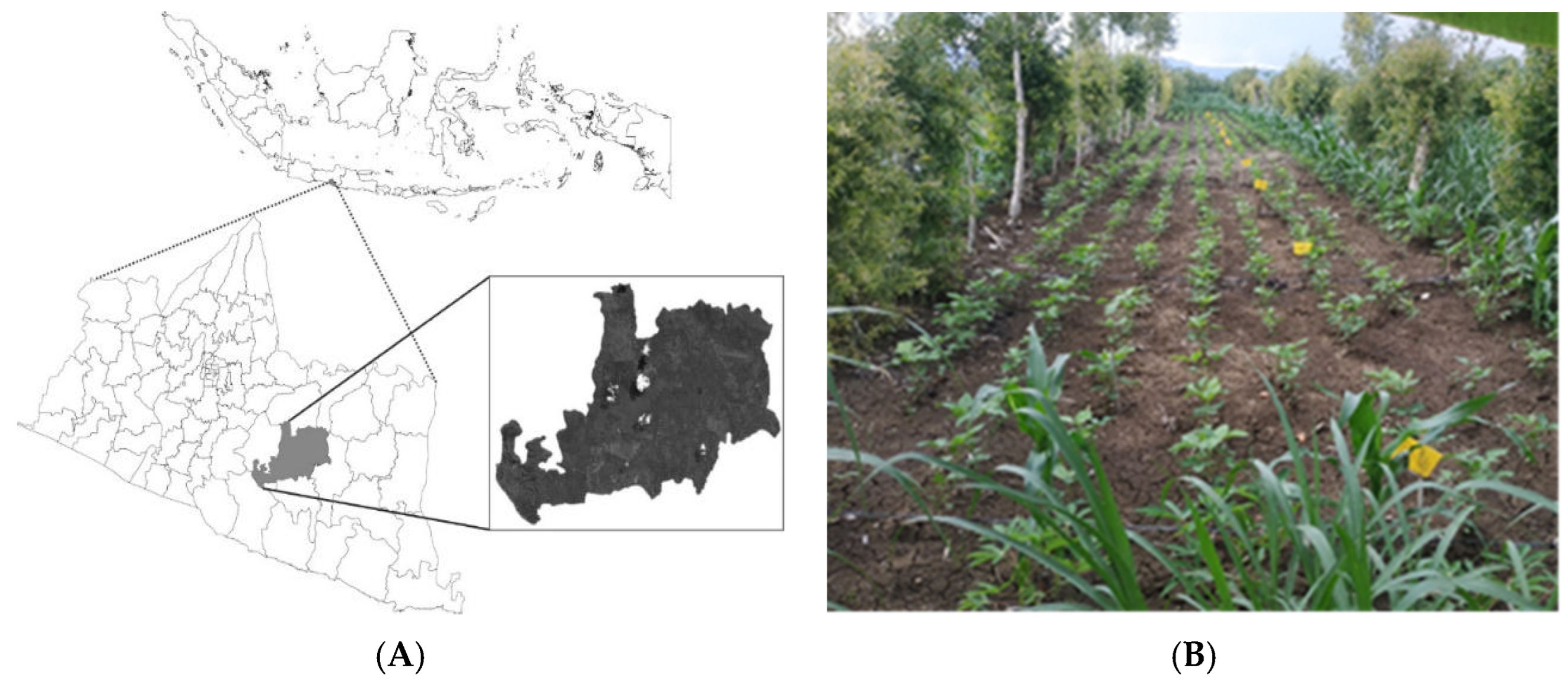
2.1. Study Sites

A two-year experiment was conducted during the dry season (March–June 2021) and the wet season (November 2021–February 2022) at Menggoran Forest Resort, Playen District, Gunungkidul Regency, Special Province of Yogyakarta, Indonesia. The experimental site was approximately 43 km to the southeast of Yogyakarta City with an altitude of approximately 150 m above sea levels (Figure 1A) [8,26,27,28]. The total rainfall, average air temperature, relative humidity, and sun hours were 586 mm, 24.80 °C, 85.00%, and 7.78 h, respectively, during the dry season and 1117 mm, 24.58 °C, 87.25%, and 7.23 h, respectively, during the wet season.

2.2. Multi-Environmental Trial Setup and Crop Management

All the trials in dry and wet seasons were laid out in a randomized complete block design factorial with three blocks as replications. The first factor was crop rotation models consisting of soybean planting after fallow (F–S), soybean planting after maize (M–S), soybean planting after rice (R–S), and continuous soybean planting (S–S). The second factor consisted of 15 major soybean cultivars that were primarily used by farmers in rainfed areas at Gunungkidul Regency (Table 1). Seeds were obtained from the Indonesian Legumes and Tuber Crops Research Institute in Malang Regency of East Java, Indonesia, and the Indonesian Center for Agricultural Biotechnology and Genetic Resource Research and Development, Bogor Regency of West Java, Indonesia. More details regarding pedigree, yield potential, harvest age, resistance level to pests and diseases, and their specific features are presented in Table 2 [29,30].

The experimental plots were placed between the kayu putih stands. The plot size was 12 m² (4 m × 3 m), with a 0.5 and 1 m distance between blocks and plots, respectively, (Figure 1B). The harvest area for soybean was 7 m², excluding border crops [7]. Soil tillage was carried out with minimum tillage. The standard spacing was 40 cm × 20 cm with two seeds per planting hole and 5 cm planting depth. Planting was completed by direct seeding in the area. In addition, 50 kg ha⁻¹ of urea, 100 kg ha⁻¹ of SP-36, and 150 kg ha⁻¹ of KCl were used as fertilizer and applied once a week after planting (wap) [28]. Irrigation was not carried out during the study, as the experimental plots were situated in rainfed areas.

2.3. Data Collection

2.3.1. Soil Characteristics

The observed parameters included % soil texture (clay, sand, and silt) [31], bulk density [31], soil moisture content [31], permeability [31], pH H₂O [32], soil organic carbon (SOC) [32], cation exchange capacity [32], electrical conductivity [32], total nitrogen [32], soil nutrient availability (phosphorus, potassium, sodium, calcium, manganese, iron, aluminum, total bacteria, and fungi) [32,33]. Such parameters were analyzed at the initial stage of the study. The observations were carried out at the study site and at the Laboratory of General Soil and Microbiology, Faculty of Agriculture, Universitas Gadjah Mada, Yogyakarta, Indonesia.

2.3.2. Soybean Yield

Seed weight data per plot were collected for each treatment in the harvest area (7 m²). The observation of soybean yield was carried out when 80% of the pods had turned yellow. The seed weight was weighed using a digital scale (Merk: ACIS Digital Precision Balance; Series: AD-600i). The seed moisture content was measured using a moisture tester (Model: TK100S Moisture Meter). The seed weight was converted to a moisture content of 12% using the following formula [7]:

$${\mathrm{yield} (\mathrm{tons} \mathrm{ha}}^{-1})=\frac{10000}{\mathrm{HA}} \times \frac{100 - \mathrm{MC}}{100 - 12} \times \mathrm{Y},$$

(1)

where yield is the yield of soybean (tons ha⁻¹); HA is the harvest area (7 m²); MC is the seed moisture content during harvesting, and Y is the seed weight during harvesting.

2.4. Statistical Analysis

The model built in this experiment was shown as follows [17,26]:

Soybean Cultivars × (Crop Rotation Models/Replicate) = Crop Rotation Models: Replicate + Soybean Cultivars + Soybean Cultivars • Crop Rotation Models,

(2)

where fixed and random effects are shown before and after the colon; the dot between the two factors represents the cross-effect; the interaction between soybean cultivars and the crop rotation model is denoted by C•M (Table 1). The random effect on the covariance structure for each treatment factor is described as follows:

i

The covariance structure for replicate (R) is $G_R={\oplus }_{j=1}^J{G}_{R\left(j\right)}$, where $G_{R\left(j\right)}$ is a diagonal matrix with diagonal elements ${\sigma }_{R\left(j\right)}^2$. A certain soil type variance was assumed.

ii

The covariance structure for the cultivar effect is the identity structure, that is, $G_{\mathrm{V}}={\sigma }^2{\rm I}$.

iii

The residual covariance structure is heterogeneous with soil-type-specific $R={\oplus }_{j=1}^J{R}_j$, where $R_j$ is a diagonal matrix with ${\sigma }_{\epsilon \left(j\right)}^2$.

Table 1. Factors for the analysis of soybean cultivars and crop rotation models in rainfed agroforestry system by using linear mixed models.

Factors	Total	Symbol
Cultivar	15	C
Crop rotation model	4	M
Replicate	3	R

Table 1. Factors for the analysis of soybean cultivars and crop rotation models in rainfed agroforestry system by using linear mixed models.

Factors	Total	Symbol
Cultivar	15	C
Crop rotation model	4	M
Replicate	3	R

The stability assessment of soybean cultivars was carried out by constructing a linear model for the C•M variance based on the cultivars. We can borrow information from crop rotation models to estimate the effect of cultivars on each crop rotation model in the dry and wet seasons. C and C•M were considered random effects. This estimation was performed using the EBLUP method because cultivars have random effects. The term ‘empirical’ was used because the components of the variance are unknown; therefore, they must be estimated [34]. The base model was reparameterized by removing the main C effect, and the C•M effect was removed using C as the subject effect to apply a variance–covariance (VCOV) model that differs from the C•M term. The genetic effect for crop rotation models was C•M for the same cultivar and correlated among crop rotation models [13,22,23,24,25].

In assessing cultivar stability, the model was generalized on the basis of the variance stability model [35]. Random effects were used to estimate cultivar effects per crop rotation model by borrowing information across crop rotation models using C and C•M effects. EBLUP and Shukla models used PROC MIXED in SAS 9.4 [36].

The GEI interpretation was visualized using the GGE biplot [16]. This technique can be used to determine the (1) which-won-where pattern in genotype and environment, (2) AEC based on environmental scaling of the mean value and stability of genotype, and (3) ranking of entries based on mean and instability. The GGE biplot was analyzed using Genstat 18th edition [37].

Table 2. Fifteen evaluated soybean cultivars (with some features).

No.	Cultivars	Pedigree	Yield Potential (tons ha−1)	Harvest Age (dap)	Pest or Disease Resistance	Specific Features
1.	Anjasmoro	Mass selection for ‘Mansuria’ pure line	2.03–2.25	82.5–92.5	Moderate resistance to leaf rust	Resistance to pod shattering
2.	Argomulyo	Introduction from Thailand	1.5–2.0	80–82	Tolerant to leaf rust	Suitable for soy milk ingredient
3.	Baluran	AVRDC Cross	2.5–3.5	80	–	–
4.	Biosoy I	The pedigree selection from a population of mutant strains from crosses of Chinese soybeans with Japanese soybeans irradiated with a dose of 250 Gray gamma rays	3.3	83	Resistance to leaf rust, pod borer, and army worm	Resistance to pod shattering
5.	Burangrang	Pure-line selection from Jember landrace	1.6–2.5	80–82	Tolerant to leaf rust	Suitable for soy milk, tempeh, and tofu
6.	Dega I	Single cross of ‘Grobogan’ and ‘Malabar’	3.82	69–73	Moderate resistance to leaf rust and not resistant to army worm	Adaptive in paddy fields
7.	Dena I	Single cross of ‘Agromulyo’ × IAC 100	2.9	78	Resistance to leaf rust, not resistant to pod borer and army worm	Tolerant to 50% shade
8.	Dena II	Single cross of IAC 100 × ‘Ijen’	2.8	81	Resistance to leaf rust and pod borer, moderate resistance to army worm	Very tolerant to 50% shade
9.	Dering I	Single cross of ‘Davros’ × MLG 2984	2.8	81	Resistance to pod borer and resistance to leaf rust	Resistance to drought in reproductive phase
10.	Dering II	Single cross of Arg/GCP–335 × ‘Baluran’	3.32	70–76	Moderate resistance to leaf, army worm, and leaf rust	Resistance to drought in reproductive phase
11.	Dering III	Single cross of ‘Dering I’ × ‘Malabar’	2.99	70–76	Moderate resistance to leaf, army worm, and leaf rust	Resistance to drought in reproductive phase
12.	Devon I	Derived from ‘Kawi’ × IAC100	2.75	83	Resistance to leaf rust and moderate resistance to pod sucker	High isoflavone content (2219.8 µg g−1)
13.	Grobogan	Pure-line selection from ‘Malabar’ in Grobogan	2.77	76	–	Less pod shattering
14.	Mahameru	Mass selection for ‘Man–suria’ pure line	2.04–2.16	83.5–94.8	Moderate resistance to leaf rust	Resistance to pod shattering
15.	Tanggamus	Hibrida (single cross): ‘Kerinci’ × No. 3911	1.22	85	Moderate resistance to leaf rust	Resistance to pod shattering, adaptive in acid dry land

Table 2. Fifteen evaluated soybean cultivars (with some features).

No.	Cultivars	Pedigree	Yield Potential (tons ha−1)	Harvest Age (dap)	Pest or Disease Resistance	Specific Features
1.	Anjasmoro	Mass selection for ‘Mansuria’ pure line	2.03–2.25	82.5–92.5	Moderate resistance to leaf rust	Resistance to pod shattering
2.	Argomulyo	Introduction from Thailand	1.5–2.0	80–82	Tolerant to leaf rust	Suitable for soy milk ingredient
3.	Baluran	AVRDC Cross	2.5–3.5	80	–	–
4.	Biosoy I	The pedigree selection from a population of mutant strains from crosses of Chinese soybeans with Japanese soybeans irradiated with a dose of 250 Gray gamma rays	3.3	83	Resistance to leaf rust, pod borer, and army worm	Resistance to pod shattering
5.	Burangrang	Pure-line selection from Jember landrace	1.6–2.5	80–82	Tolerant to leaf rust	Suitable for soy milk, tempeh, and tofu
6.	Dega I	Single cross of ‘Grobogan’ and ‘Malabar’	3.82	69–73	Moderate resistance to leaf rust and not resistant to army worm	Adaptive in paddy fields
7.	Dena I	Single cross of ‘Agromulyo’ × IAC 100	2.9	78	Resistance to leaf rust, not resistant to pod borer and army worm	Tolerant to 50% shade
8.	Dena II	Single cross of IAC 100 × ‘Ijen’	2.8	81	Resistance to leaf rust and pod borer, moderate resistance to army worm	Very tolerant to 50% shade
9.	Dering I	Single cross of ‘Davros’ × MLG 2984	2.8	81	Resistance to pod borer and resistance to leaf rust	Resistance to drought in reproductive phase
10.	Dering II	Single cross of Arg/GCP–335 × ‘Baluran’	3.32	70–76	Moderate resistance to leaf, army worm, and leaf rust	Resistance to drought in reproductive phase
11.	Dering III	Single cross of ‘Dering I’ × ‘Malabar’	2.99	70–76	Moderate resistance to leaf, army worm, and leaf rust	Resistance to drought in reproductive phase
12.	Devon I	Derived from ‘Kawi’ × IAC100	2.75	83	Resistance to leaf rust and moderate resistance to pod sucker	High isoflavone content (2219.8 µg g−1)
13.	Grobogan	Pure-line selection from ‘Malabar’ in Grobogan	2.77	76	–	Less pod shattering
14.	Mahameru	Mass selection for ‘Man–suria’ pure line	2.04–2.16	83.5–94.8	Moderate resistance to leaf rust	Resistance to pod shattering
15.	Tanggamus	Hibrida (single cross): ‘Kerinci’ × No. 3911	1.22	85	Moderate resistance to leaf rust	Resistance to pod shattering, adaptive in acid dry land

3. Results

3.1. Soil Characteristic in Study Sites

The soil at the study site was Lithic Haplusterts [8,17,26]. Lithic Haplusterts had a limestone rock and ustic soil moisture regime, and it belonged to the Vertisol order, which had a shallow solum (<30 cm) and rock contact. Lithic Haplusterts will shrink (cracks: width > 5 mm and thickness > 25 cm) and expand under dry and wet conditions [38].

Soil analysis carried out before the study on various crop rotations models in the dry and wet seasons is shown in Table 3. The soil texture was dominated by clay and it had very slow permeability (0.01 cm h⁻¹). In the wet season (25.35–27.53 mm cm⁻¹), the soil water content was higher than that in the dry season (16.45–19.77 mm cm⁻¹). The pH of H₂O, SOC, CEC, and EC in various crop rotations models in the wet and dry seasons were slightly alkaline, low, very high, and low, respectively.

The total N content in the soil varied from very low to moderate levels. The total N, which was at a moderate level in continuous soybean (S–S) in the dry season was 0.25%, and soybean planting after fallow (F–S) and continuous soybeans (S–S) in the wet season were 0.22% and 0.29%, respectively. The available P content varied from low to moderate, ranging from 8 to 18 ppm. The available base cations (K, Na, Ca, and Mg) at various crop rotation models and seasons were categorized as low, medium, and high. The Mn, Fe, and Al availability in all crop rotations and seasons were included in the very low category.

Soil biology was represented by the total bacteria and fungi in the soil. In general, in the wet season, the total bacteria and fungi were higher than those in the dry season. The results of the land suitability evaluation for soybeans in the research location were included in the marginally suitable category.

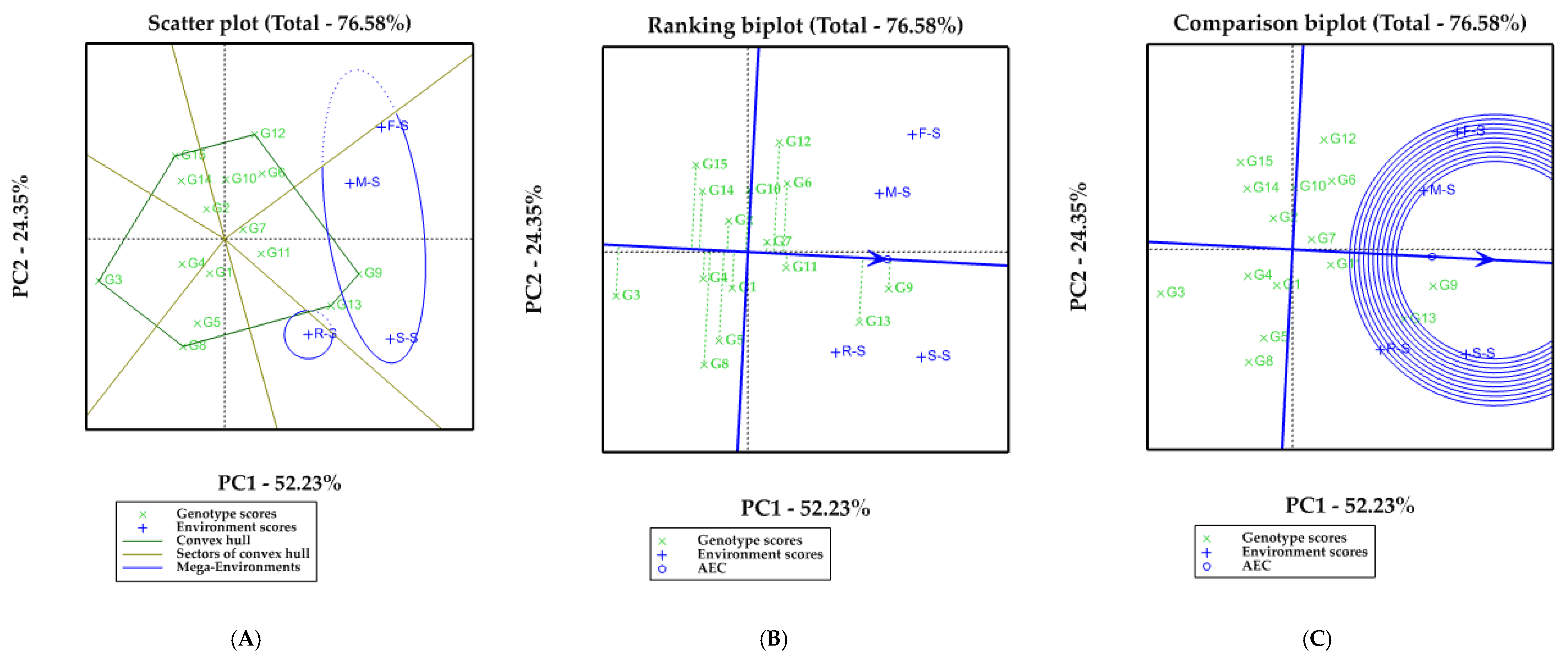
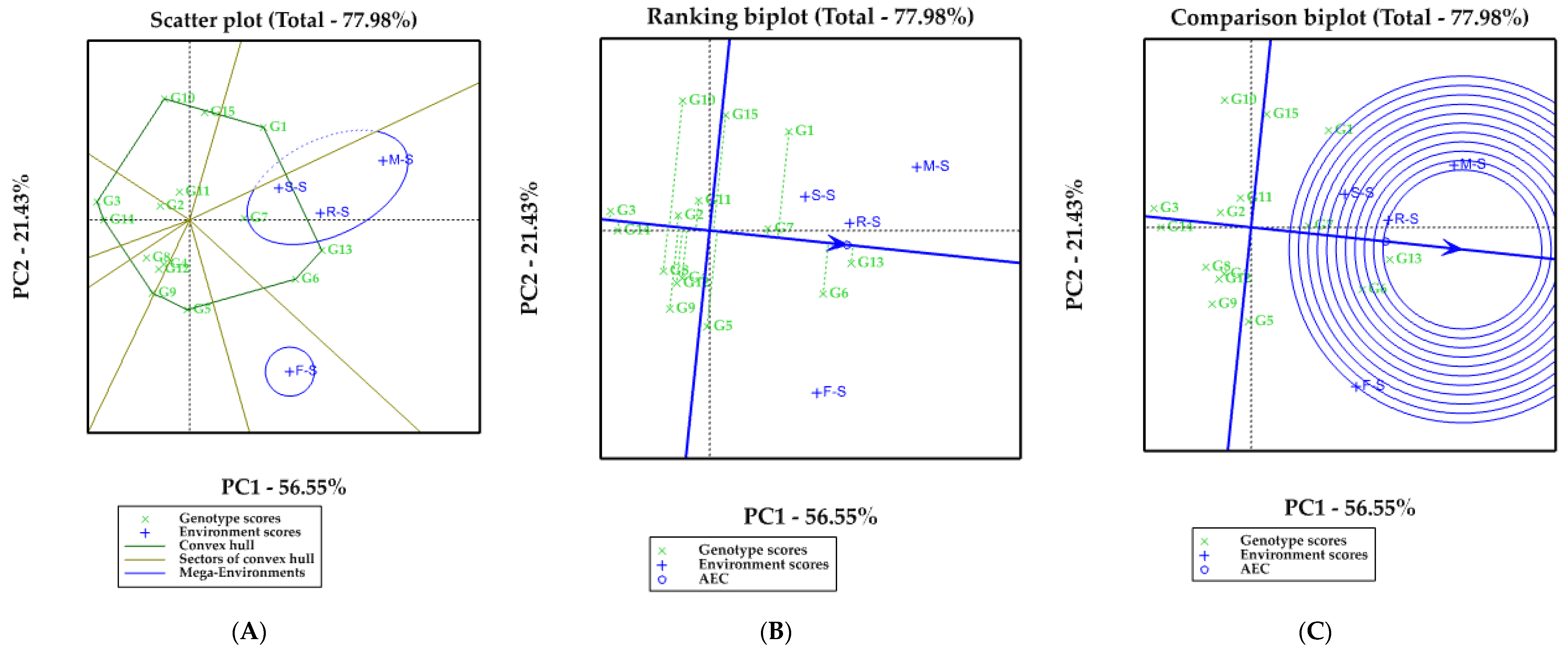
3.2. Ranking and EBLUP of 15 Soybean Cultivars in Each Crop Rotation Model

The C•M model was a term from the VCOV model evaluated using Akaike information criterion (AIC) values, including independent (ID), compound symmetry (CS), heterogeneous compound symmetry (CSH), and unstructured (UN, Table 4). Based on the AIC value, the CS model was the most suitable because it had the lowest AIC value compared with ID, CSH, and UN. The lowest AIC value in the CS model with relatively few cultivars was used as the basis for presenting EBLUP for the CS model. In this study, the genetic correlation between the dry and wet seasons was relatively small; thus, differences in soybean yields and ranking in various crop rotation models were observed (Table 5).

The prediction and ranking of soybean yield in different cultivars and crop rotation models were conducted using the EBLUP of the C•S effect (Table 6 and Table 7). Based on the EBLUP, different patterns regarding the performance of soybean cultivars were observed in various crop rotation models and seasons. Based on the crop rotation model, the Dering I cultivar showed the highest yield in F−S during the dry season of 1.267 tons ha⁻¹, followed by the Dega I and Dena I cultivars with yields of 1.250 and 1.222 tons ha⁻¹, respectively. By contrast, the Dena II cultivar had the lowest yield in F−S of 0.754 tons ha⁻¹.

Table 3. Soil characteristics (physical, chemical, and biological) in study sites.

No.	Soil Characteristics	Unit	Crop Rotation Models
			Dry Season				Wet Season
			F−S	M−S	R−S	S−S	F−S	M−S	R−S	S−S
	Soil Physical
1.	Soil Texture	–	Clay	Clay	Clay	Clay	Clay	Clay	Clay	Clay
2.	Bulk Density	g cm−3	1.16	1.12	1.11	1.12	1.11	1.12	1.15	1.09
3.	Soil Moisture Content	mm cm−1	16.45	17.18	19.21	19.77	25.35	26.46	27.14	27.53
4.	Permeability	cm h−1	0.001	0.01	0.01	0.01	0.01	0.01	0.01	0.01
	Soil Chemical
1.	pH H2O	–	8.4	8.3	8.2	8.1	8.3	8.1	8.0	8.0
2.	Soil Organic Carbon	%	1.6	1.5	1.6	1.4	1.7	1.6	1.6	1.5
3.	Cation Exchange Capacity	cmol(+) kg−1	62.23	58.48	59.72	59.92	64.71	63.72	64.82	64.51
4.	Electrical Conductivity	dS m−1	1.682	1.689	1.614	1.647	1.711	1.742	1.691	1.708
5.	Total Nitrogen	%	0.09	0.16	0.18	0.25	0.22	0.19	0.16	0.29
6.	Soil Nutrient Availability:
	− Phosphorus	mg L	9	11	11	12	11	18	8	17
	− Potassium	cmol(+) kg−1	0.18	0.12	0.15	0.11	0.26	0.22	0.22	0.24
	− Sodium	cmol(+) kg−1	0.64	0.62	0.61	0.59	0.74	0.69	0.67	0.65
	− Calcium	cmol(+) kg−1	29.72	24.46	25.67	24.89	23.11	23.01	21.38	22.71
	− Magnesium	cmol(+) kg−1	1.27	1.16	1.18	1.11	1.34	1.26	1.62	1.42
	− Manganese	mg L−1	1.14	2.22	1.19	2.16	1.92	1.12	1.93	1.11
	− Fe	mg L−1	1.28	1.13	1.22	1.16	1.19	1.11	1.16	1.08
	− Al	mg L−1	1.54	1.42	1.32	1.31	1.27	1.19	1.13	1.09
	Soil Biological
1.	Total Bacteria	cfu	1.32 × 105	1.74 × 105	1.92 × 105	1.82 × 105	1.99 × 105	2.53 × 105	1.64 × 105	2.31 × 105
2.	Total Fungi	cfu	1.46 × 103	1.61 × 103	1.71 × 103	1.68 × 103	1.83 × 103	1.94 × 103	1.57 × 103	1.90 × 103

Table 3. Soil characteristics (physical, chemical, and biological) in study sites.

No.	Soil Characteristics	Unit	Crop Rotation Models
			Dry Season				Wet Season
			F−S	M−S	R−S	S−S	F−S	M−S	R−S	S−S
	Soil Physical
1.	Soil Texture	–	Clay	Clay	Clay	Clay	Clay	Clay	Clay	Clay
2.	Bulk Density	g cm−3	1.16	1.12	1.11	1.12	1.11	1.12	1.15	1.09
3.	Soil Moisture Content	mm cm−1	16.45	17.18	19.21	19.77	25.35	26.46	27.14	27.53
4.	Permeability	cm h−1	0.001	0.01	0.01	0.01	0.01	0.01	0.01	0.01
	Soil Chemical
1.	pH H2O	–	8.4	8.3	8.2	8.1	8.3	8.1	8.0	8.0
2.	Soil Organic Carbon	%	1.6	1.5	1.6	1.4	1.7	1.6	1.6	1.5
3.	Cation Exchange Capacity	cmol(+) kg−1	62.23	58.48	59.72	59.92	64.71	63.72	64.82	64.51
4.	Electrical Conductivity	dS m−1	1.682	1.689	1.614	1.647	1.711	1.742	1.691	1.708
5.	Total Nitrogen	%	0.09	0.16	0.18	0.25	0.22	0.19	0.16	0.29
6.	Soil Nutrient Availability:
	− Phosphorus	mg L	9	11	11	12	11	18	8	17
	− Potassium	cmol(+) kg−1	0.18	0.12	0.15	0.11	0.26	0.22	0.22	0.24
	− Sodium	cmol(+) kg−1	0.64	0.62	0.61	0.59	0.74	0.69	0.67	0.65
	− Calcium	cmol(+) kg−1	29.72	24.46	25.67	24.89	23.11	23.01	21.38	22.71
	− Magnesium	cmol(+) kg−1	1.27	1.16	1.18	1.11	1.34	1.26	1.62	1.42
	− Manganese	mg L−1	1.14	2.22	1.19	2.16	1.92	1.12	1.93	1.11
	− Fe	mg L−1	1.28	1.13	1.22	1.16	1.19	1.11	1.16	1.08
	− Al	mg L−1	1.54	1.42	1.32	1.31	1.27	1.19	1.13	1.09
	Soil Biological
1.	Total Bacteria	cfu	1.32 × 105	1.74 × 105	1.92 × 105	1.82 × 105	1.99 × 105	2.53 × 105	1.64 × 105	2.31 × 105
2.	Total Fungi	cfu	1.46 × 103	1.61 × 103	1.71 × 103	1.68 × 103	1.83 × 103	1.94 × 103	1.57 × 103	1.90 × 103

Table 4. Akaike information criterion (AIC) for variance–covariance structures fitted to cultivars by crop rotation models.

Model	Akaike Information Criterion
	Dry Season	Wet Season
Identity	1292.7	1400.8
Compound symmetry	1312.7	1420.8
Heteroscedastic compound symmetry	1314.1	1422.1
Unstructured	1319.8	1427.9

Table 4. Akaike information criterion (AIC) for variance–covariance structures fitted to cultivars by crop rotation models.

Model	Akaike Information Criterion
	Dry Season	Wet Season
Identity	1292.7	1400.8
Compound symmetry	1312.7	1420.8
Heteroscedastic compound symmetry	1314.1	1422.1
Unstructured	1319.8	1427.9

In soybean planting after maize (M−S), the Grobogan, Dering I, and Devon I cultivars had the highest yields of 1.200, 1.174, and 1.155 tons ha⁻¹, respectively. On the contrary, the Baluran cultivar had the lowest yield of 0.736 tons ha⁻¹. The crop rotation model using soybean planting after rice (R−S) model showed that soybean yields ranging from grades 1 to 3 were represented by the Dering I, Grobogan, and Anjasmoro cultivars with yields of 1.375, 1.334, and 1.306 tons ha⁻¹, respectively. By contrast, Devon I had the lowest yield of 0.984 tons ha⁻¹. In continuous soybean (S−S), the Grobogan cultivar had the highest yield of 1.349 tons ha⁻¹, followed by the Dering I and Dering III cultivars with yields of 1.346 and 1.210 tons ha⁻¹, respectively, whereas the Baluran cultivar had the lowest yield of 0.789 tons ha⁻¹. Therefore, the best crop rotation model for soybean cultivars in the dry season was R−S > S−S > F−S > M−S.

Table 5. Variance estimates (10⁻¹ kg² ha⁻²) for the C•M model.

Effect †	Group	Variance Estimate
		Dry Season	Wet Season
R	F–S	0.00107	0.00565
	M–S	0.00078	0.00645
	R–S	0.00089	0.00383
	S–S	0.00105	0.00494
C•M ‡	Genetic variance (C)	0.15450	0.20173
	Genetic correlation §	0.08066	0.11877
E	F–S	0.00003	0.00005
	M–S	0.00002	0.00007
	R–S	0.00316	0.00005
	S–S	0.00003	0.00026

† R: Replicate; C•M: Cultivar-by-crop rotation model interaction; E: error term/residual. ‡ Obtained by fitting the C•M model. § The unit does not apply for genetic correlation.

Table 5. Variance estimates (10⁻¹ kg² ha⁻²) for the C•M model.

Effect †	Group	Variance Estimate
		Dry Season	Wet Season
R	F–S	0.00107	0.00565
	M–S	0.00078	0.00645
	R–S	0.00089	0.00383
	S–S	0.00105	0.00494
C•M ‡	Genetic variance (C)	0.15450	0.20173
	Genetic correlation §	0.08066	0.11877
E	F–S	0.00003	0.00005
	M–S	0.00002	0.00007
	R–S	0.00316	0.00005
	S–S	0.00003	0.00026

† R: Replicate; C•M: Cultivar-by-crop rotation model interaction; E: error term/residual. ‡ Obtained by fitting the C•M model. § The unit does not apply for genetic correlation.

The different wet season patterns related to soybean yield are shown in Table 6. The crop rotation model in F−S showed that the Grobogan cultivar had the highest yield of 2.187 tons ha⁻¹, followed by the Dega I and Burangrang cultivars with 2.175 and 2.128 tons ha⁻¹, respectively. On the contrary, the Dering II cultivar had the lowest yield of 1.611 tons ha⁻¹. The Grobogan, Anjasmoro, and Dena I cultivars had the highest yields in M−S with 2.435, 2.388, and 2.354 tons ha⁻¹, respectively, whereas the Mahameru cultivar had the lowest yield of 1.733 tons ha⁻¹. The R−S results showed that the Dega I cultivar had the highest yield of 2.049, followed by the Grobogan and Argomulyo cultivars with yields of 1.895 and 1.772 tons ha⁻¹, respectively. By contrast, the Mahameru cultivar had the lowest yield in R−S of 1.449 tons ha⁻¹. In S−S, the Grobogan, Anjasmoro, and Dega I cultivars had the highest yields of 2.247, 2.233, and 2.202 tons ha⁻¹, respectively, whereas the Baluran cultivar had the lowest yield of 1.851 tons ha⁻¹. Therefore, the best crop rotation model for soybean cultivars in the wet season was M−S > S−S > F−S > R−S. A difference in the productivity of soybean cultivars was observed between dry and wet seasons. In the dry season, the highest productivity was dominated by the Dering I and Grobogan cultivars, whereas in the wet season, it is dominated by the Grobogan and Dega I cultivars.

3.3. Stability Variance Estimates

Visualization using the GGE biplot in the dry season on all crop rotation models formed six sectors, and only two contained mega-environments (Mega-E, Figure 2A). The outermost genotype forms a polygon connected by the convex hull line in the sector. The genotype that forms the polygon was known as the vertex genotype, which consisted of Baluran (G3), Dena II (G8), Dering I (G9), Devon I (G12), Grobogan (G13), and Tanggamus (G15) cultivars (Figure 2A). Vertex genotype indicates that the genotype had the highest or lowest yield in some or all crop rotation models.

The first Mega-E consisted of three environments, namely, soybean planting after fallow (F−S), soybean planting after maize (M−S), and continuous soybean (S−S) crop rotation models. The second Mega-E consisted of one environment, namely, the soybean planting after rice (R−S) crop rotation model. Mega-E had one genotype, namely, the Dering I cultivar, which consisted of F−S, M−S, M–S, and S–S. Thus, the Dering I cultivar had the best performance on F−S, M−S, and S−S crop rotations models. The second Mega-E consisted of R−S, which showed that no genotype had the best performance.

Evaluation related to the stability of soybean cultivars was performed using the AEC (Figure 2B). The AEC showed the GGE biplot based on environmental scaling of the mean value and stability of the genotype. The AEC was bounded by two lines, namely, the biplot abscissa and biplot ordinate. The abscissa biplot line showed the yield performance of soybean genotypes, whereas the ordinate biplot line divided genotypes that had a high average yield (right side) and low yields (left side). Soybean cultivars that were included in the high average yield category in all crop rotation models during the dry season included Dering I (G9), Grobogan (G13), Dering III (G11), Dega I (G6), Dena I (G7), Devon I (G12), and Dering II (G10). The length of the line between the genotype and biplot abscissa indicated the level of stability of a genotype. The short line indicated high stability, whereas the long line indicated low stability. In general, the Dering I cultivar showed a high yield performance, which was relatively stable in all crop rotation models in the dry season.

The ideal genotype in all crop rotation models in the dry season was determined using the GGE biplot based on the genotype focus scale to compare the genotype with the ideal genotype. A genotype is ideal if it has a high yield and stability (Figure 2C). It is important because the ideal genotype can be recommended to farmers. The ideal genotype is found in the first concentric circle, whereas the genotype in the second concentric circle can be categorized as the desired genotype. Furthermore, the third concentric circle can be categorized as an unwanted genotype because it has a low mean yield and stability. The Dering I cultivar belonged to the first concentric circle; thus, the Dering I cultivar could be categorized as an ideal genotype. By contrast, no desired genotype was identified for the second concentric circle. Therefore, only Dering I was recommended for all crop rotation models in the dry season.

Visualization using the GGE biplot in the wet season on all crop rotation models shows eight sectors, and only two had Mega-E (Figure 3A). Vertex genotypes consisted of cultivars Anjasmoro (G1), Baluran (G3), Burangrang (G5), Dega I (G6), Dering I (G9), Dering II (G10), Grobogan (G13), Mahameru (G14), and Tanggamus (G15). The first Mega-E consisted of three crop rotation models, namely, soybean planting after maize (M−S), soybean planting after soybean (R−S), and continuous soybean (S−S). The second Mega-E consisted of one environment: soybean planting after fallow (F−S). In these two Mega-E, neither of the two genotypes had the best performance. Based on the AEC, soybean cultivars Grobogan (G13), Dega I (G6), Anjasmoro (G1), Dena I (G7), Burangrang (G5), and Tanggamus (G15) were included in the high average yield category in all crop rotation models in successive wet seasons. In general, Grobogan cultivars showed a high yield performance, and they were relatively stable in all crop rotation models during the wet season (Figure 3B).

The GGE biplot based on genotype-focused scaling to compare genotypes with ideal genotypes indicated that the Grobogan cultivar was identified in the first concentric circle (Figure 3C). The Grobogan cultivar can be categorized as an ideal genotype, whereas no desired genotype was identified in the second concentric circle. Therefore, only the Grobogan cultivar was recommended for all crop rotation models in the wet season.

Table 6. Ranking and empirical best linear unbiased prediction (tons ha⁻¹) of 15 soybean cultivars in each crop rotation model during the wet season.

Ranking	Fallow–Soybean (F–S)		Maize–Soybean (M–S)		Rice–Soybean (R–S)		Soybean–Soybean (S–S)
	Cultivars	EBLUP	Cultivars	EBLUP	Cultivars	EBLUP	Cultivars	EBLUP
1	Dering I	1.267	Grobogan	1.200	Dering I	1.375	Grobogan	1.349
2	Dega I	1.250	Dering I	1.174	Grobogan	1.334	Dering I	1.346
3	Dena I	1.222	Devon I	1.155	Anjasmoro	1.306	Dering III	1.210
4	Devon I	1.204	Anjasmoro	1.153	Burangrang	1.279	Dena II	1.179
5	Grobogan	1.096	Argomulyo	1.144	Dega I	1.270	Burangrang	1.065
6	Dering II	1.093	Dega I	1.080	Dena I	1.269	Dena I	1.021
7	Dering III	1.084	Dering II	1.069	Biosoy I	1.164	Devon I	1.021
8	Tanggamus	1.077	Mahameru	1.049	Baluran	1.138	Dering II	1.001
9	Mahameru	0.974	Dering III	1.015	Dering III	1.117	Biosoy I	0.969
10	Argomulyo	0.935	Tanggamus	0.939	Dena II	1.113	Argomulyo	0.966
11	Biosoy I	0.921	Biosoy I	0.908	Argomulyo	1.066	Anjasmoro	0.934
12	Burangrang	0.906	Dena II	0.880	Dering II	1.034	Dega I	0.931
13	Anjasmoro	0.853	Dena I	0.853	Mahameru	1.009	Mahameru	0.886
14	Baluran	0.758	Burangrang	0.838	Tanggamus	0.994	Tanggamus	0.844
15	Dena II	0.754	Baluran	0.736	Devon I	0.984	Baluran	0.789

Table 6. Ranking and empirical best linear unbiased prediction (tons ha⁻¹) of 15 soybean cultivars in each crop rotation model during the wet season.

Ranking	Fallow–Soybean (F–S)		Maize–Soybean (M–S)		Rice–Soybean (R–S)		Soybean–Soybean (S–S)
	Cultivars	EBLUP	Cultivars	EBLUP	Cultivars	EBLUP	Cultivars	EBLUP
1	Dering I	1.267	Grobogan	1.200	Dering I	1.375	Grobogan	1.349
2	Dega I	1.250	Dering I	1.174	Grobogan	1.334	Dering I	1.346
3	Dena I	1.222	Devon I	1.155	Anjasmoro	1.306	Dering III	1.210
4	Devon I	1.204	Anjasmoro	1.153	Burangrang	1.279	Dena II	1.179
5	Grobogan	1.096	Argomulyo	1.144	Dega I	1.270	Burangrang	1.065
6	Dering II	1.093	Dega I	1.080	Dena I	1.269	Dena I	1.021
7	Dering III	1.084	Dering II	1.069	Biosoy I	1.164	Devon I	1.021
8	Tanggamus	1.077	Mahameru	1.049	Baluran	1.138	Dering II	1.001
9	Mahameru	0.974	Dering III	1.015	Dering III	1.117	Biosoy I	0.969
10	Argomulyo	0.935	Tanggamus	0.939	Dena II	1.113	Argomulyo	0.966
11	Biosoy I	0.921	Biosoy I	0.908	Argomulyo	1.066	Anjasmoro	0.934
12	Burangrang	0.906	Dena II	0.880	Dering II	1.034	Dega I	0.931
13	Anjasmoro	0.853	Dena I	0.853	Mahameru	1.009	Mahameru	0.886
14	Baluran	0.758	Burangrang	0.838	Tanggamus	0.994	Tanggamus	0.844
15	Dena II	0.754	Baluran	0.736	Devon I	0.984	Baluran	0.789

Table 7. Ranking and empirical best linear unbiased prediction (tons ha⁻¹) of 15 soybean cultivars in each crop rotation model during the dry season.

Ranking	Fallow–Soybean (F–S)		Maize–Soybean (M–S)		Rice–Soybean (R–S)		Soybean–Soybean (S–S)
	Cultivars	EBLUP	Cultivars	EBLUP	Cultivars	EBLUP	Cultivars	EBLUP
1	Grobogan	2.187	Grobogan	2.435	Dega I	2.049	Grobogan	2.247
2	Dega I	2.175	Anjasmoro	2.388	Grobogan	1.895	Anjasmoro	2.233
3	Burangrang	2.128	Dena I	2.354	Argomulyo	1.772	Dega I	2.202
4	Dering I	2.024	Dega I	2.206	Anjasmoro	1.761	Tanggamus	2.163
5	Dena I	2.019	Tanggamus	2.159	Tanggamus	1.756	Burangrang	2.162
6	Devon I	1.989	Dering II	2.158	Dering III	1.755	Mahameru	2.145
7	Biosoy I	1.981	Biosoy I	2.063	Baluran	1.596	Dering II	2.125
8	Dena II	1.941	Dering III	1.970	Dena I	1.586	Dering III	2.107
9	Anjasmoro	1.816	Dering I	1.967	Burangrang	1.578	Dena I	2.093
10	Dering III	1.806	Argomulyo	1.953	Dering I	1.535	Devon I	2.091
11	Argomulyo	1.794	Burangrang	1.943	Biosoy I	1.524	Dena II	2.073
12	Mahameru	1.786	Devon I	1.922	Devon I	1.521	Argomulyo	1.892
13	Baluran	1.697	Dena II	1.891	Dena II	1.510	Biosoy I	1.853
14	Tanggamus	1.669	Baluran	1.776	Dering II	1.485	Dering I	1.853
15	Dering II	1.611	Mahameru	1.733	Mahameru	1.449	Baluran	1.851

Table 7. Ranking and empirical best linear unbiased prediction (tons ha⁻¹) of 15 soybean cultivars in each crop rotation model during the dry season.

Ranking	Fallow–Soybean (F–S)		Maize–Soybean (M–S)		Rice–Soybean (R–S)		Soybean–Soybean (S–S)
	Cultivars	EBLUP	Cultivars	EBLUP	Cultivars	EBLUP	Cultivars	EBLUP
1	Grobogan	2.187	Grobogan	2.435	Dega I	2.049	Grobogan	2.247
2	Dega I	2.175	Anjasmoro	2.388	Grobogan	1.895	Anjasmoro	2.233
3	Burangrang	2.128	Dena I	2.354	Argomulyo	1.772	Dega I	2.202
4	Dering I	2.024	Dega I	2.206	Anjasmoro	1.761	Tanggamus	2.163
5	Dena I	2.019	Tanggamus	2.159	Tanggamus	1.756	Burangrang	2.162
6	Devon I	1.989	Dering II	2.158	Dering III	1.755	Mahameru	2.145
7	Biosoy I	1.981	Biosoy I	2.063	Baluran	1.596	Dering II	2.125
8	Dena II	1.941	Dering III	1.970	Dena I	1.586	Dering III	2.107
9	Anjasmoro	1.816	Dering I	1.967	Burangrang	1.578	Dena I	2.093
10	Dering III	1.806	Argomulyo	1.953	Dering I	1.535	Devon I	2.091
11	Argomulyo	1.794	Burangrang	1.943	Biosoy I	1.524	Dena II	2.073
12	Mahameru	1.786	Devon I	1.922	Devon I	1.521	Argomulyo	1.892
13	Baluran	1.697	Dena II	1.891	Dena II	1.510	Biosoy I	1.853
14	Tanggamus	1.669	Baluran	1.776	Dering II	1.485	Dering I	1.853
15	Dering II	1.611	Mahameru	1.733	Mahameru	1.449	Baluran	1.851

The results of the GGE biplot using the AEC were strengthened by stability analysis using the Shukla model (Table 8). This model showed that the effect of C•M was highly variable among cultivars. The smaller the variance of each cultivar, the more stable it was. If the value was 0, then the cultivar was considered stable because the variance was negative. The more significant the variance of each cultivar, the more unstable the crop rotation model. Soybean cultivars that were fairly stable in the dry season included Dering I (0.708), Mahameru (0.210), Argomulyo (0.630), and Dering II (0.708, Table 8). During the wet season, the relatively stable soybean cultivars included Dena II (0.000) and Grobogan (0.026), whereas the fairly stable cultivar was Devon I (0.537, Table 8).

Table 8. Stability variance estimates (10⁻¹ kg² ha⁻²) for the Shukla model.

Cultivars	Stability Variance Estimate For C•S
	Dry Season	Wet Season
Anjasmoro	2.742	7.684
Argomulyo	0.630	3.330
Baluran	6.454	3.706
Biosoy I	1.161	2.129
Burangrang	3.085	11.214
Dega I	1.887	9.584
Dena I	2.892	4.768
Dena II	5.120	0.000
Dering I	0.176	1.708
Dering II	0.708	4.789
Dering III	1.393	1.983
Devon I	1.114	0.537
Grobogan	4.054	0.026
Mahameru	0.210	1.695
Tanggamus	5.163	5.053

Table 8. Stability variance estimates (10⁻¹ kg² ha⁻²) for the Shukla model.

Cultivars	Stability Variance Estimate For C•S
	Dry Season	Wet Season
Anjasmoro	2.742	7.684
Argomulyo	0.630	3.330
Baluran	6.454	3.706
Biosoy I	1.161	2.129
Burangrang	3.085	11.214
Dega I	1.887	9.584
Dena I	2.892	4.768
Dena II	5.120	0.000
Dering I	0.176	1.708
Dering II	0.708	4.789
Dering III	1.393	1.983
Devon I	1.114	0.537
Grobogan	4.054	0.026
Mahameru	0.210	1.695
Tanggamus	5.163	5.053

4. Discussion

The C•M model, which was a term for the VCOV model, uses a reparameterized base model without using the main effects of cultivars. In this case, the C•M effect uses a different VCOV model with C as the subject. The specific genetic effects of the C•M crop rotation models for cultivars are the same and correlated among crop rotation models. Thus, the BLUP for specific crop rotation models can borrow strength/information from certain crop rotation models [13,23,25,39]. In this study, soybean yields varied widely in various crop rotation models in dry and wet seasons. This result is due to the low genetic correlation among environments [13].

The multiple symmetry (CS) model is recommended in this study compared with the unstructured (UN) model. The number of soybean cultivars is not large; thus, it is not supported when using a more complex heteroscedastic model. In addition, the CS model had the smallest AIC value compared with other VCOV structures. The unstructured model had a high AIC value, and different covariances can cause this model to be overfitted and not parsimonious enough. Stroup et al. [34] reported that the simple model is considered a parsimonious model.

The CS model assumed the genetic variance among crop rotation models; therefore, yield stability was used to estimate genetic variance and covariance. Kleinknecht et al. [25] reported that the CS model was used to analyze maize data in India. In this study, the genetic correlation between the dry and wet seasons was relatively small; thus, differences in soybean yields and ratings were observed among various crop rotation models. Considering that the terms C and C•S are random, strength/information could be borrowed from a particular crop rotation model. Smith et al. [40] suggested that in selecting the best cultivar, the predicted cultivar effect must match the actual cultivar.

The difference in soybean yield in various crop rotation models in the wet and dry seasons was due to the high GEI. Kasno and Trustinah [41] indicated that the soybean yield is generally inconsistent in various environments because of an interaction between genotype × season × location. Each genotype responds differently to fertilizers and soil amendments, causing yield differences [42,43]. This result is consistent with soil analysis results in this study on various crop rotation models and seasons. The Dering I and Grobogan cultivars had the highest yields in the dry season. The Dering I cultivar had the highest yield in F–S and R–S because it is sensitive to Mn, which is relatively low in F–S and R–S [26,44]. In addition, the Dering I cultivar is resistant to drought during the reproductive phase [30].

The Grobogan cultivar had a relatively high yield in the dry season in addition to the Dering I cultivar. Alam et al. [44] stated that the increase in the Grobogan cultivar yield is followed by an increase in N and P content in the soil, which is consistent with the higher N content in M–S and S–S than in F–S and R–S in the dry season. In the wet season, the highest yields in various crop rotation models were dominated by the Grobogan and Dega I cultivars, followed by the Anjasmoro cultivar. The Grobogan cultivar is highly adaptive in soils with high available Ca and P content. The Dega I cultivar is adaptive in paddy fields, whereas the Anjasmoro is fairly stable in Lithic Haplusterts soil [8,26,27,30].

Crop rotation is a proven management strategy to increase crop yields significantly, which provides many important benefits for improving soil and yields’ physical, chemical, and biological properties. For soil biological properties, the application of crop rotation can increase the heterogeneity and abundance of bacteria and fungi communities [10]. Continuous cropping systems without legumes are not recommended because the yield and soil health are not sustainable [45].

In the dry season, the highest mean yield of soybean cultivars was observed in soybean planting after rice (R–S), whereas in the wet season, it was observed in soybean planting after maize (M–S). Agomoh et al. [46] suggested that soybean yield decreased when planted continuously but increased by 39–44% when planted alternately with cereal crops. This result is related to soil’s higher C content and microbial activity. In this study, the content of SOC in R–S in the dry season and M–S in the wet season was relatively higher when compared to other crop rotation models of 1.6% and 1.7%, respectively. In the dry season, R–S has 1.92 × 10⁵ cfu and 1.71 × 10³ cfu for bacteria and fungi, whereas M–S in the wet season has 2.53 × 10⁵ cfu and 1.94 × 10³ cfu. The total number of bacteria and fungi was relatively higher than in other crop rotation models in each season.

5. Conclusions

The cultivars that are well suited to the environment can maximize the yield potential of these cultivars and help to build a sustainable production system. In the dry season, the Dering I cultivar had the highest yields in F–S and R–S of 1.267 and 1.375 tons ha⁻¹, whereas the Grobogan cultivar had the highest yield in M–S and S–S of 1.200 and 1.349 tons ha⁻¹. In the wet season, the Grobogan cultivar showed the highest yields in F–S, M–S, and S–S of 2.187, 2.435, and 2.247 tons ha⁻¹, respectively, whereas the Dega I cultivar had the highest yield in R–S of 2.049 tons ha⁻¹. The Dering I cultivar was found to be fairly stable, whereas the Grobogan cultivar tended to be relatively unstable in the dry and wet seasons for all crop rotation models. We recommended the use of the Dering I cultivar on the F–S and R–S crop rotation models and the Grobogan cultivar on the M–S and S–S crop rotation models in the dry season, whereas the use of the Grobogan cultivar was recommended on all crop rotation models in the wet season, particularly in rainfed agroforestry systems with kayu putih.

References

1. Ministry of Agriculture. The Strategic Plan of Ministry of Agriculture for 2015–2019; Ministry of Agriculture: Jakarta, Indonesia, 2016. Available online: http://sakip.pertanian.go.id/admin/file/Renstra%20Kementan%202015–2019%20(edisi%20revisi).pdf (accessed on 25 May 2022).
2. FAO. The Future of Food and Agriculture–Trends and Challenges; The Food and Agriculture Organization (FAO): Rome, Italy, 2017; Available online: https://www.fao.org/3/i6583e/i6583e.pdf (accessed on 25 May 2022).
3. Ministry of Agriculture. Indonesian Soybean Production Projection (2020–2024); Ministry of Agriculture: Jakarta, Indonesia, 2021. Available online: https://databoks.katadata.co.id/datapublish/2021/06/04/produksi–kedelai–diproyeksi–turun–hingga–2024#:~:text=Proyeksi%20Produksi%20Kedelai%20Indonesia%20(2020%2D2024)&text=Pada%20tahun%20ini%2C%20proyeksi%20kedelai,6%20ribu%20ton%20pada%202022 (accessed on 25 May 2022).
4. Statistics Indonesia. The Harvested Area and Rice Production in Indonesia 2019; Statistics Indonesia: Jakarta, Indonesia, 2020. Available online: https://www.bps.go.id/pressrelease/2020/02/04/1752/luas–panen–dan–produksi–padi–pada–tahun–2019–mengalami–penurunan–dibandingkan–tahun–2018–masing–masing–sebesar–6–15–dan–7–76–persen.html (accessed on 25 May 2022).
5. Mulyani, A.; Nursyamsi, D.; Syakir, M. Land resource utilization strategy to achieve sustainable rice self–sufficiency. J. Sumberd. Lahan 2017, 11, 11–22. [Google Scholar] [CrossRef]
6. Alam, T.; Suryanto, P.; Kurniasaih, B.; Kastono, D.; Supriyanta; Widyawan, M.H.; Muttaqin, A.S.; Taryono. Kayu putih forest: Window opportunity for food estate development in Indonesia. In Appropriate Technology 75th Faculty of Agriculture Serving; Deviyanti, J., Ed.; Lily Publisher: Yogyakarta, Indonesia, 2021; pp. 144–146. [Google Scholar]
7. Alam, T.; Suryanto, P.; Susyanto, N.; Kurniasih, B.; Basunanda, P.; Putra, E.T.S.; Kastono, D.; Respatie, D.W.; Widyawan, M.H.; Nurmansyah; et al. Performance of 45 non–linear models for determining critical period of weed control and acceptable yield loss in soybean agroforestry systems. Sustainability 2022, 14, 7636. [Google Scholar] [CrossRef]
8. Suryanto, P.; Faridah, E.; Nurjanto, H.H.; Putra, E.T.S.; Kastono, D.; Handayani, S.; Boy, R.; Widyawan, M.H.; Alam, T. Short–term effect of in situ biochar briquettes on nitrogen loss in hybrid rice grown in an agroforestry system for three years. Agronomy 2022, 12, 564. [Google Scholar] [CrossRef]
9. FAO. Drought Characteristics and Management in Central Asia and Turkey; The Food and Agriculture Organization (FAO) Sub–regional Office for Central Asia, Ankara, Turkey and Land and Water Division: Rome, Italy, 2017; Available online: https://www.fao.org/3/i6738e/i6738e.pdf (accessed on 25 May 2022).
10. Bowles, T.M.; Mooshammer, M.; Socolar, Y.; Calderón, F.; Cavigelli, M.A.; Culman, S.W.; Deen, W.; Drury, C.F.; Garcia, A.G.Y.; Gaudin, A.C.M.; et al. Long–term evidence shows that crop–rotation diversification increases agricultural resilience to adverse growing conditions in North America. One Earth 2020, 2, 284–293. [Google Scholar] [CrossRef]
11. Neupane, A.; Bulbul, I.; Wang, Z.; Lehman, R.M.; Nafziger, E.; Marzano, S.Y.L. Long term crop rotation effect on subsequent soybean yield explained by soil and root-associated microbes and soil health indicators. Sci. Rep. 2021, 11, 9200. [Google Scholar] [CrossRef]
12. Dolijanović, Z.; Milena, S. The role of the crop rotation in maize agroecosystem sustainability. In Zea mays L.: Molecular Genetics, Potential Environmental Effects and Impact on Agricultural Practices; Barnes, L., Ed.; Nova Science Publishers, Inc.: New York, NY, USA, 2016. [Google Scholar]
13. Piepho, H.P.; Nazir, M.F.; Qamar, M.; Rattu, A.U.R.; Hussain, M.; Ahmad, G.; Ahmad, J.; Laghari, K.B.; Vistro, I.A.; Kakar, M.S.; et al. Stability analysis for a countrywide series of wheat trials in Pakistan. Crop Sci. 2016, 56, 2465–2475. [Google Scholar] [CrossRef]
14. Eberhart, S.A.; Russell, W.A. Stability parameters for comparing varieties. Crop Sci. 1966, 6, 36–40. [Google Scholar] [CrossRef]
15. Finlay, K.W.; Wilkinson, G.N. The analysis of adaptation in a plant breeding programme. Aust. J. Agric. Res. 1963, 14, 742–754. [Google Scholar] [CrossRef]
16. Yan, W.; Kang, M.S.; Ma, B.; Woods, S.; Cornelius, P.L. GGE–biplot vs. AMMI analysis of genotype–by–environment data. Crop Sci. 2007, 47, 643–655. [Google Scholar] [CrossRef]
17. Alam, T.; Suryanto, P.; Supriyanta; Basunanda, P.; Wulandari, R.A.; Kastono, D.; Widyawan, M.H.; Nurmansyah, T. Rice cultivar selection in an agroforestry system through GGE biplot and EBLUP. Biodiversitas 2021, 22, 4750–4757. [Google Scholar] [CrossRef]
18. Yan, W.; Kang, M.S. GGE Biplot Analysis: A Graphical Tool for Breeders, Geneticists and Agronomists, 1st ed.; CRC Press: Boca Raton, FL, USA, 2019; p. 286. [Google Scholar]
19. Bilgin, O.; Guzmán, C.; Baser, I.; Crossa, J.; Korkut, K.Z.; Balkan, A. Evaluation of grain yield and quality traits of bread wheat genotypes cultivated in Northwest Turkey. Crop Sci. 2015, 56, 73–84. [Google Scholar] [CrossRef]
20. Gerrano, A.S.; van Rensburg, W.S.J.; Mathew, I.; Shayanowako, A.I.T.; Bairu, M.W.; Venter, S.L.; Swart, W.; Mofokeng, A.; Mellem, J.; Labuschagne, M. Genotype and genotype × environment interaction effects on the grain yield performance of cowpea genotypes in dryland farming system in South Africa. Euphytica 2020, 216, 80. [Google Scholar] [CrossRef]
21. Oladosu, Y.; Rafii, M.Y.; Abdullah, N.; Magaji, U.; Miah, G.; Hussin, G.; Ramli, A. Genotype × environment interaction and stability analyses of yield and yield components of established and mutant rice genotypes tested in multiple locations in Malaysia. Acta Agric. Scand. Sect. B–Soil Plant Sci. 2017, 67, 590–606. [Google Scholar] [CrossRef]
22. Buntaran, H.; Forkman, J.; Piepho, H.P. Projecting results of zoned multi-environment trials to new locations using environmental covariates with random coefcient models: Accuracy and precision. Theor. App. Genet. 2021, 134, 1513–1530. [Google Scholar] [CrossRef] [PubMed]
23. Buntaran, H.; Piepho, H.P.; Hagman, J.; Forkman, J. A cross–validation of statistical models for zoned–based prediction in cultivar testing. Crop Sci. 2019, 59, 1544–1553. [Google Scholar] [CrossRef]
24. Buntaran, H.; Piepho, H.P.; Schmidt, P.; Ryden, J.; Halling, M.; Forkman, J. Cross–validation of stagewise mixed–model analysis of Swedish variety trials with winter wheat and spring barley. Crop Sci. 2020, 60, 2221–2240. [Google Scholar] [CrossRef]
25. Kleinknecht, K.; Möhring, J.; Singh, K.P.; Zaidi, P.H.; Atlin, G.N.; Piepho, H.P. Comparison of the performance of BLUE and BLUP for zoned Indian maize data. Crop Sci. 2013, 53, 1384–1391. [Google Scholar] [CrossRef]
26. Alam, T.; Kurniasih, B.; Suryanto, P.; Basunanda, P.; Supriyanta; Ambarwati, E.; Widyawan, M.H.; Handayani, S.; Taryono. Stability analysis for soybean in agroforestry system with kayu putih. SABRAO J. Breed. Genet. 2019, 51, 405–418. [Google Scholar]
27. Alam, T.; Suryanto, P.; Nurmalasari, A.I.; Kurniasih, B. GGE Biplot analysis for the suitability of soybean varieties in an agroforestry system based on kayu putih (Melaleuca cajuputi) stands. Caraka Tani J. Sustain. Agric. 2019, 34, 213–222. [Google Scholar] [CrossRef]
28. Alam, T.; Suryanto, P.; Handayani, S.; Kastono, D.; Kurniasih, B. Optimizing application of biochar, compost and nitrogen fertilizer in soybean intercropping with kayu putih (Melaleuca cajuputi). Rev. Bras. Cienc. Solo 2020, 44, e0200003. [Google Scholar] [CrossRef]
29. Indonesian Center for Agricultural Biotechnology and Genetic Resource Research. Biosoy 1 Soybean; Indonesian Center for Agricultural Biotechnology and Genetic Resource Research, Ministry of Agriculture: West Java, Indonesia, 2018. Available online: http://biogen.litbang.pertanian.go.id/biosoy–1/ (accessed on 25 May 2022).
30. Mejaya, M.J.; Harnowo, D.; Adie, M.M. Technical Guidelines for Soybean Cultivation in Various Agroecosystems; Indonesian Legume and Tuber Crops Research Institute, Ministry of Agriculture: East Java, Indonesia, 2015. Available online: https://opac.perpusnas.go.id/DetailOpac.aspx?id=956412 (accessed on 25 May 2022).
31. Bandyopadhyay, K.K.; Aggarwal, P.; Chakraborty, D.; Pradhan, S.; Garg, R.N.; Singh, R. Practical Manual on Measurement of Soil Physical Properties; Division of Agricultural Physics, Indian Agricultural Research Institute: New Delhi, India, 2012; p. 62. [Google Scholar]
32. Peters, J. Wisconsin Procedures for Soil Testing, Plant Analysis and Feed & Forage Analysis; Soil Science Department, College of Agriculture and Life Sciences, University of Wisconsin: Madison, WI, USA, 2013. Available online: https://datcp.wi.gov/Documents/NMProcedures.pdf (accessed on 29 June 2022).
33. David, A.B.; Davidson, C.E. Estimation method for serial dilution experiments. J. Microbiol Methods 2014, 107, 214–221. [Google Scholar] [CrossRef] [PubMed] [Green Version]
34. Stroup, W.W.; Milliken, G.A.; Claassen, E.A.; Wolfinger, R.D. SAS® for Mixed Models: Introduction and Basic Applications; SAS Institute Inc.: Cary, NC, USA, 2018; pp. 307–338. [Google Scholar]
35. Shukla, G.K. Some statistical aspects of partitioning genotype–environmental components of variability. Heredity 1972, 29, 237–245. [Google Scholar] [CrossRef] [PubMed]
36. SAS Institute Inc. Step–by–Step Programming with Base SAS® 9.4, 2nd ed.; SAS Institute Inc.: Cary, NC, USA, 2013. [Google Scholar]
37. Goedhart, P.W.; Thissen, J.T.N.M. Biometris GenStat Procedure Library Manual, 18th ed.; Wageningen University and Research Center: Wageningen, The Netherlands, 2016. [Google Scholar]
38. Boettinger, J.; Chiaretti, J.; Ditzler, C.; Galbraith, J.; Kerschen, K.; Loerch, C.; McDanie, P.; McVey, S.; Monger, C.; Owens, P.; et al. Illustrated Guide to Soil Taxonomy, Version 2; U.S. Department of Agriculture, Natural Resources Conservation Service, National Soil Survey Center: Lincoln, NE, USA, 2015.
39. Piepho, H.P.; Möhring, J. Best linear unbiased prediction for subdivided target regions. Crop Sci. 2005, 45, 1151–1159. [Google Scholar] [CrossRef]
40. Smith, A.B.; Cullis, B.R.; Thompson, R. The analysis of crop cultivar breeding and evaluation trials: An overview of current mixed model approaches. J. Agric. Sci. 2005, 143, 449–462. [Google Scholar] [CrossRef]
41. Kasno, A.; Trustinah. Genotype–environment interaction analysis of peanut in Indonesia. SABRAO J. Breed. Genet. 2015, 47, 482–492. [Google Scholar]
42. Giller, K.E.; Tittonell, P.; Rufino, M.C.; van Wijk, M.T.; Zingore, S.; Mapfumo, P.; Adjeinsiah, S.; Herrero, M.; Chikowo, R.; Corbeels, M.; et al. Communicating complexity: Integrated assessment of trade–offs concerning soil fertility management within African farming system to support innovation and development. Agric. Syst. 2011, 104, 191–203. [Google Scholar] [CrossRef]
43. Klee, H.J.; Tieman, D.M. Genetic challenges of flavor improvement in tomato. Trends Genet. 2013, 29, 257–267. [Google Scholar] [CrossRef]
44. Alam, T.; Muhartini, S.; Suryanto, P.; Ambarwati, E.; Kastono, D.; Nurmalasari, A.I.; Kurniasih, B. Soybean varieties suitability in agroforestry system with kayu putih under influence of soil quality parameters. Rev. Ceres 2020, 67, 410–418. [Google Scholar] [CrossRef]
45. Ashworth, A.J.; Allen, F.L.; Saxton, A.M.; Tyler, D.D. Impact of crop rotations and soil amendments on long–term no–tilled soybean yield. Agron. J. 2017, 109, 938–946. [Google Scholar] [CrossRef]
46. Agomoh, I.V.; Drury, C.F.; Yang, X.; Phillips, L.A.; Reynolds, W.D. Crop rotation enhances soybean yields and soil health indicators. Soil Sci. Soc. Am. J. 2021, 5, 1185–1195. [Google Scholar] [CrossRef]
Figure 1. (A) Geographical locations of the study site (latitude 7°52′59.5992″ S to 7°59′41.1288″ S and longitude 110°26′21.462″ E to 110° 35′7.4868″ E) and (B) soybean among kayu putih stands.
Agronomy 12 02012 g001
Figure 2. Soybean crop rotation stability in the dry season. (A) GGE biplot polygon with which-won-where pattern; (B) AEC shows the GGE biplot based on environmental scaling of the mean value and stability of genotype; (C) GGE biplot based on genotype-focused scaling to compare genotypes with the ideal genotype. G1: Anjasmoro; G2: Argomulyo; G3: Baluran; G4: Biosoy I; G5: Burangrang; G6: Dega I; G7: Dena I; G8: Dena II; G9: Dering I; G10: Dering II; G11: Dering III; G12: Devon I; G13: Grobogan; G14: Mahameru; G15: Tanggamus. F–S: Soybean planting after fallow; R–M: Soybean planting after maize; R–S: Soybean planting after rice; S–S: continuous soybean.
Agronomy 12 02012 g002
Figure 3. Soybean crop rotation stability during the wet season. (A) GGE biplot polygon with which-won-where pattern; (B) AEC shows the GGE biplot based on environmental scaling of the mean value and stability of genotype; (C) GGE biplot based on genotype-focused scaling to compare genotypes with the ideal genotype. G1: Anjasmoro; G2: Argomulyo; G3: Baluran; G4: Biosoy I; G5: Burangrang; G6: Dega I; G7: Dena I; G8: Dena II; G9: Dering I; G10: Dering II; G11: Dering III; G12: Devon I; G13: Grobogan; G14: Mahameru; G15: Tanggamus. F–S: Soybean planting after fallow; R–M: Soybean planting after maize; R–S: Soybean planting after rice; S–S: continuous soybean.
Agronomy 12 02012 g003
Publisher’s Note: MDPI stays neutral with regard to jurisdictional claims in published maps and institutional affiliations.