
Irrigation Scheduling and Production of Wheat with Different Water Quantities in Surface and Drip Irrigation: Field Experiments and Modelling Using CROPWAT and SALTMED


Abstract
1. Introduction
2. Materials and Methods
2.1. Field Study Site
2.2. Experimental Layout and Design
2.3. Measurement of Soil Water Content
2.4. Measurements of Yield Components, Grain Yield, and Water Productivity
2.5. Maximum Grain Yield
2.6. CROPWAT Model
- -
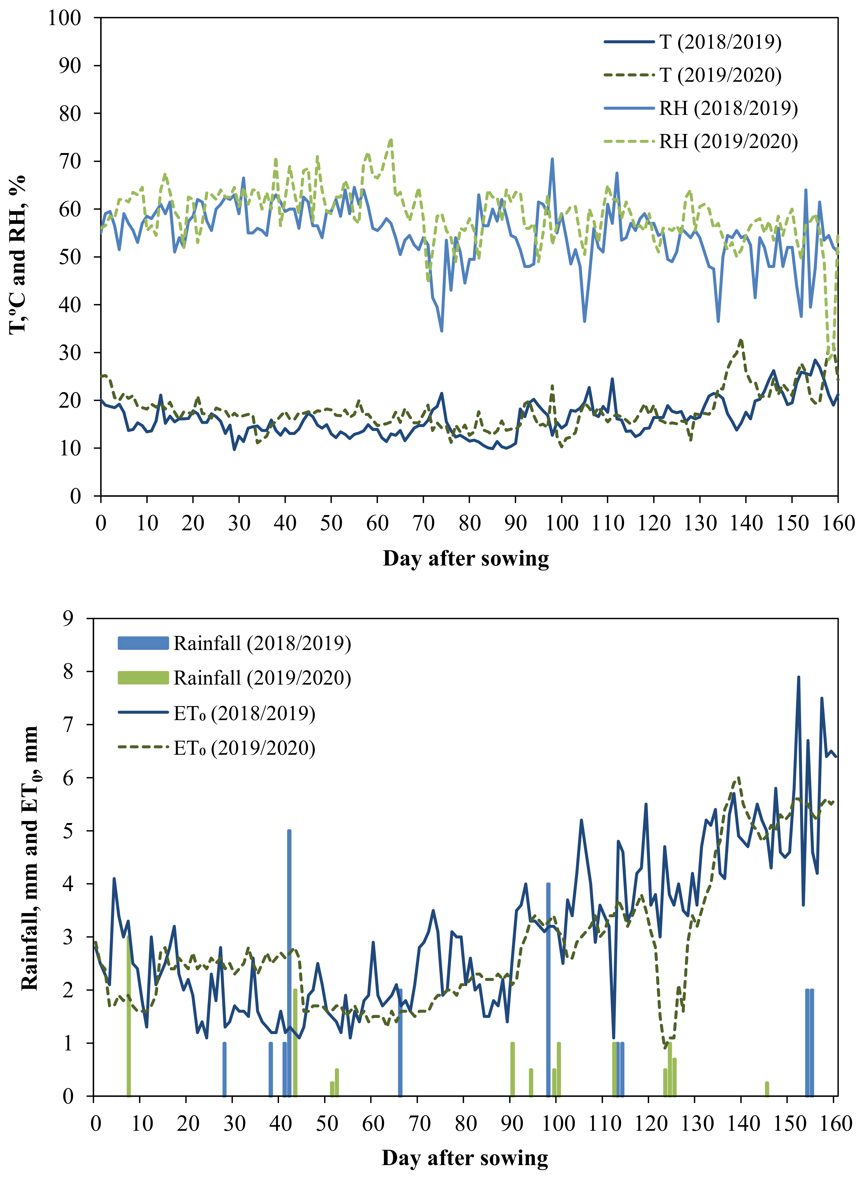
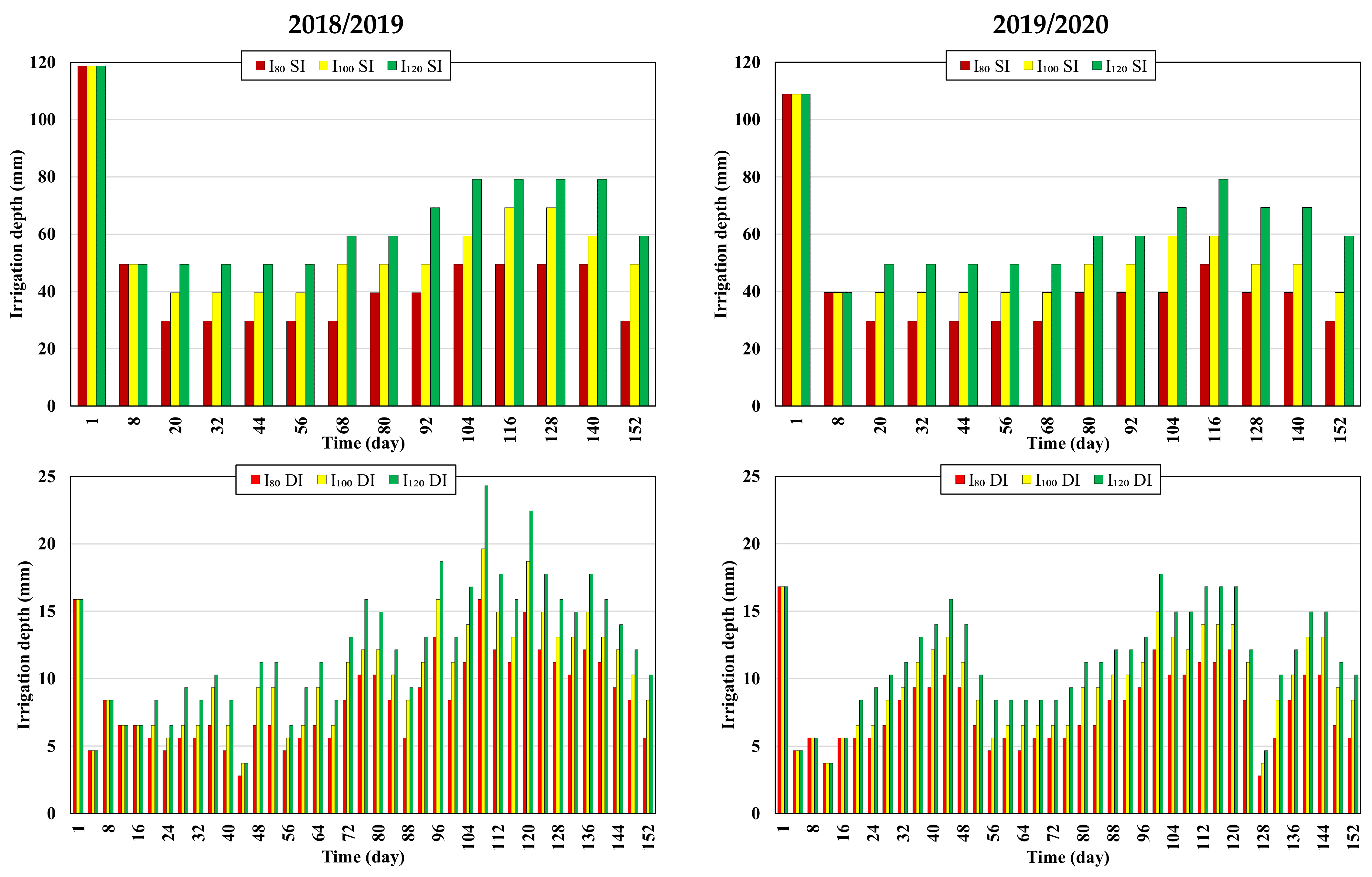
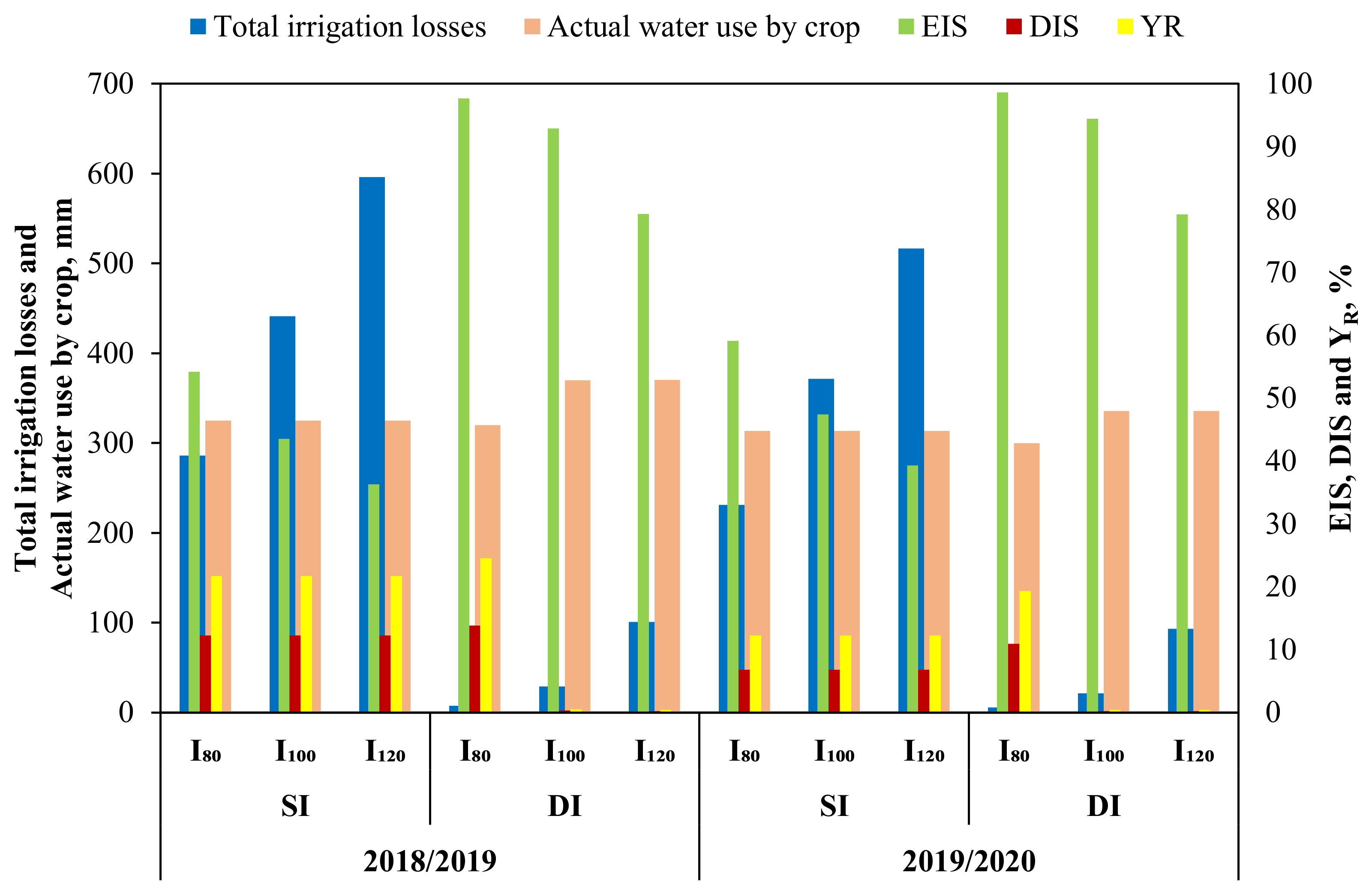
- The daily ET0 values were calculated using the Penman–Monteith FAO-56 equation (Equation (2)), which was based on climatic data from the Central Laboratory for Agricultural Climate’s Meteorological Data, as well as the daily rainfall data, for the seasons of 2018/2019 and 2019/2020. The actual crop evapotranspiration was estimated by multiplying ET0, Kc, and 0.8, 1, or 1.2. The efficiencies of SI and DI were estimated through field investigation, which was about 69% and 93%, respectively. Irrigation application depth was then estimated at irrigation events for SI and DI, as shown in Figure 2.
- -
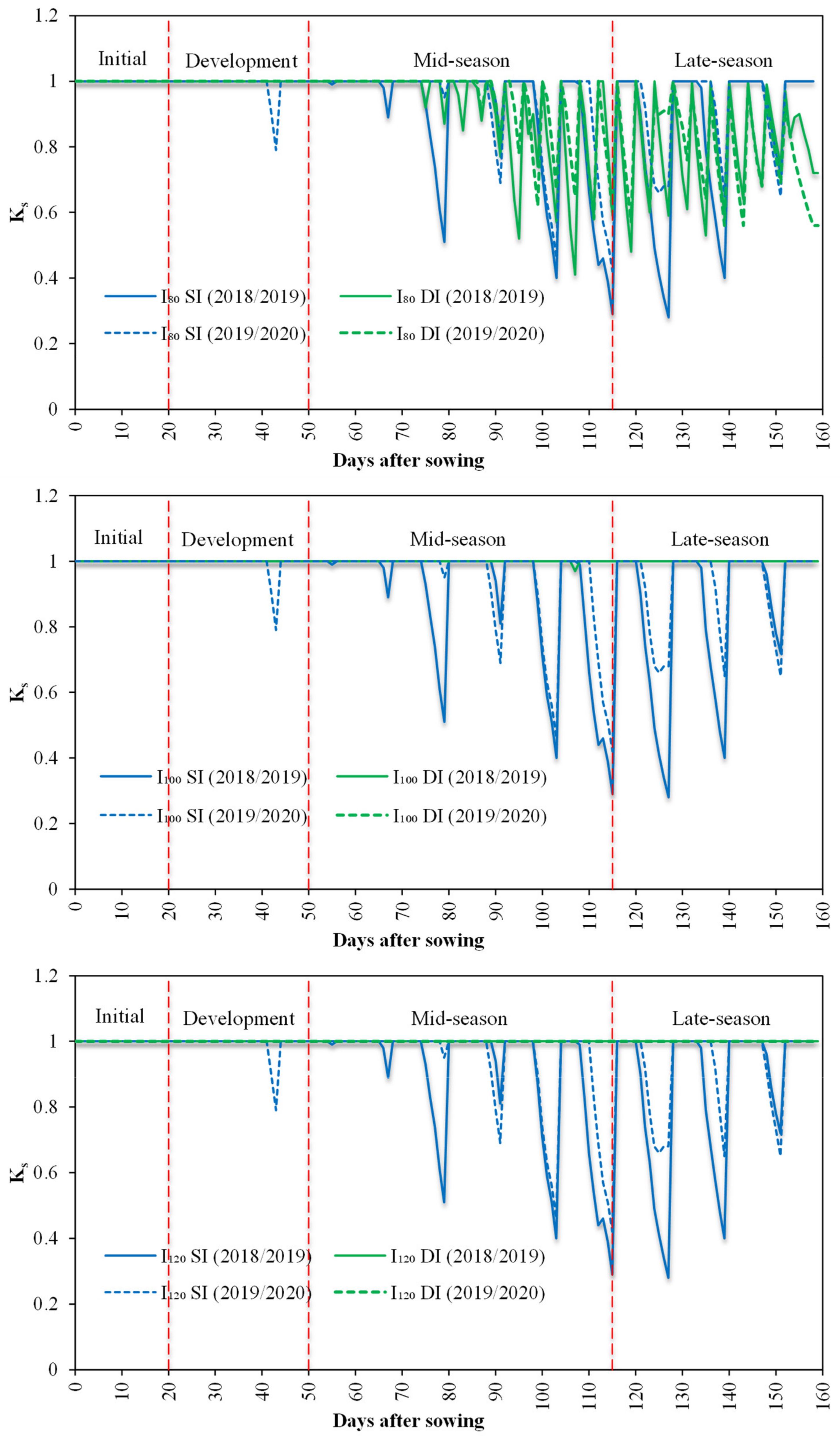
- Planting and harvesting dates, duration and water stress coefficient (Ks) of crop growth stages, and root depth were all included in the crop data. In addition, according to Allen et al. [39], the depletion fraction (p) (0.65 for initial and mid-season stages, and 0.57 for late-season stage) were calculated using the following equation:where is the depletion fraction at ETc = 5 mm/day, which is equivalent to winter wheat as 0.55 [39].
- -
- Total available soil water from measured data (Table 1), maximum rooting depth and maximum rain infiltration rate from FAO, and initial soil moisture depletion from the CROPWAT program were among the soil data.
2.7. SALTMED Model
- Climate data, including the daily data of maximum and minimum temperatures, wind speed, sunshine hours, rainfall, relative humidity, total solar radiation, and net radiation. The Penman–Monteith FAO-56 equation (Equation (2)) was used to calculate the daily ET0 values.
- Irrigation management data, including applied irrigation water amounts, dates of irrigation events, and irrigation water quality, were based on field measurement data.
- Soil parameters, including saturated SWC, initial soil moisture, saturated hydraulic conductivity, and salinity, were based on measurements either in the laboratory or in the field. Soil evaporation coefficient (Ke) values were taken from Allen et al. [39]. The Richards equation was used in the model to simulate two-dimensional water flow in the soil. The analytical functions of van Genuchten [66] in the model were used for determining soil hydraulic properties (i.e., the soil water pressure head and hydraulic conductivity relationships).
- Crop parameters, including plant height, maximum and minimum root depth, leaf area index, length of the growth stage, and sowing and harvesting dates, were obtained from field measurements. From Allen et al. [39], Kc and fraction cover (Fc) for the initial, middle, and late growth stages were taken. Basal crop coefficient (Kcb) values were then estimated as:
2.8. Performance Accuracy Criteria
2.9. Statistical Analysis
3. Results and Discussion
3.1. Irrigation Water Applied
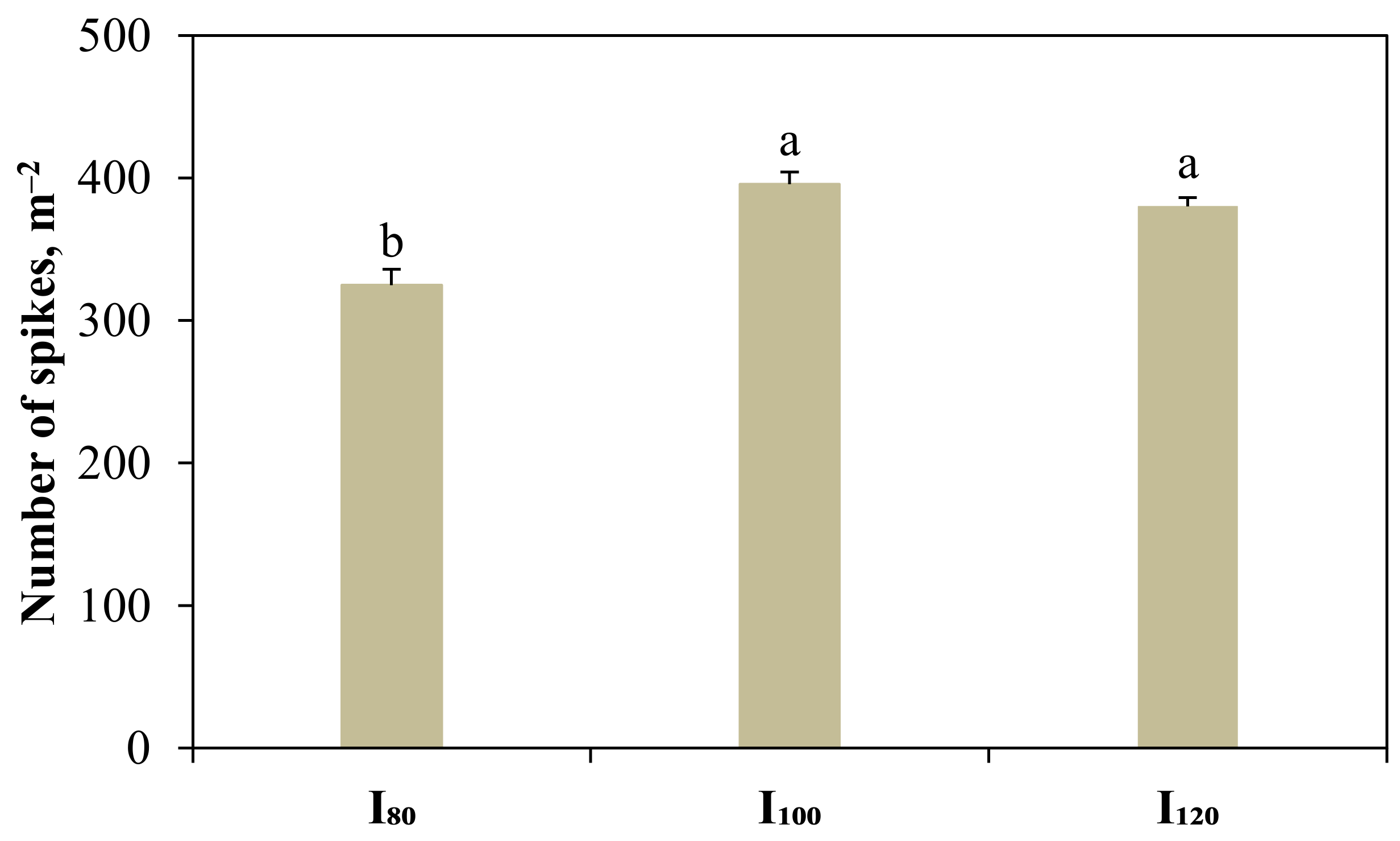
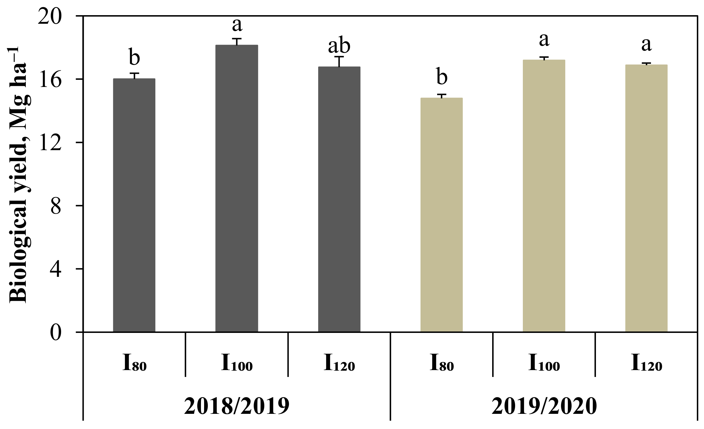
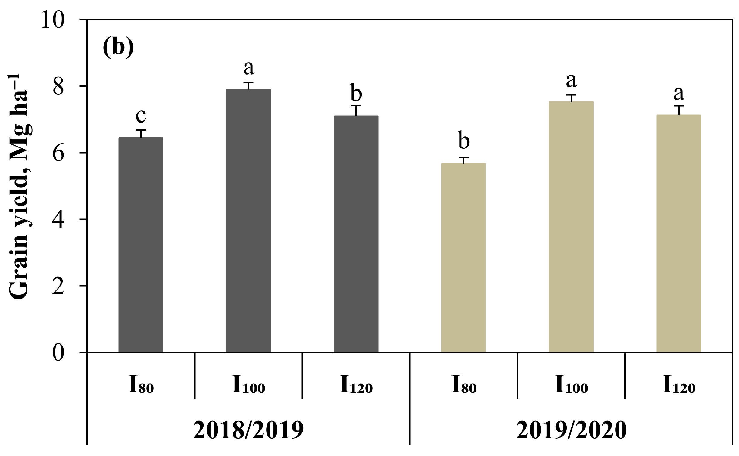
3.2. Yield Components and Grain Yield
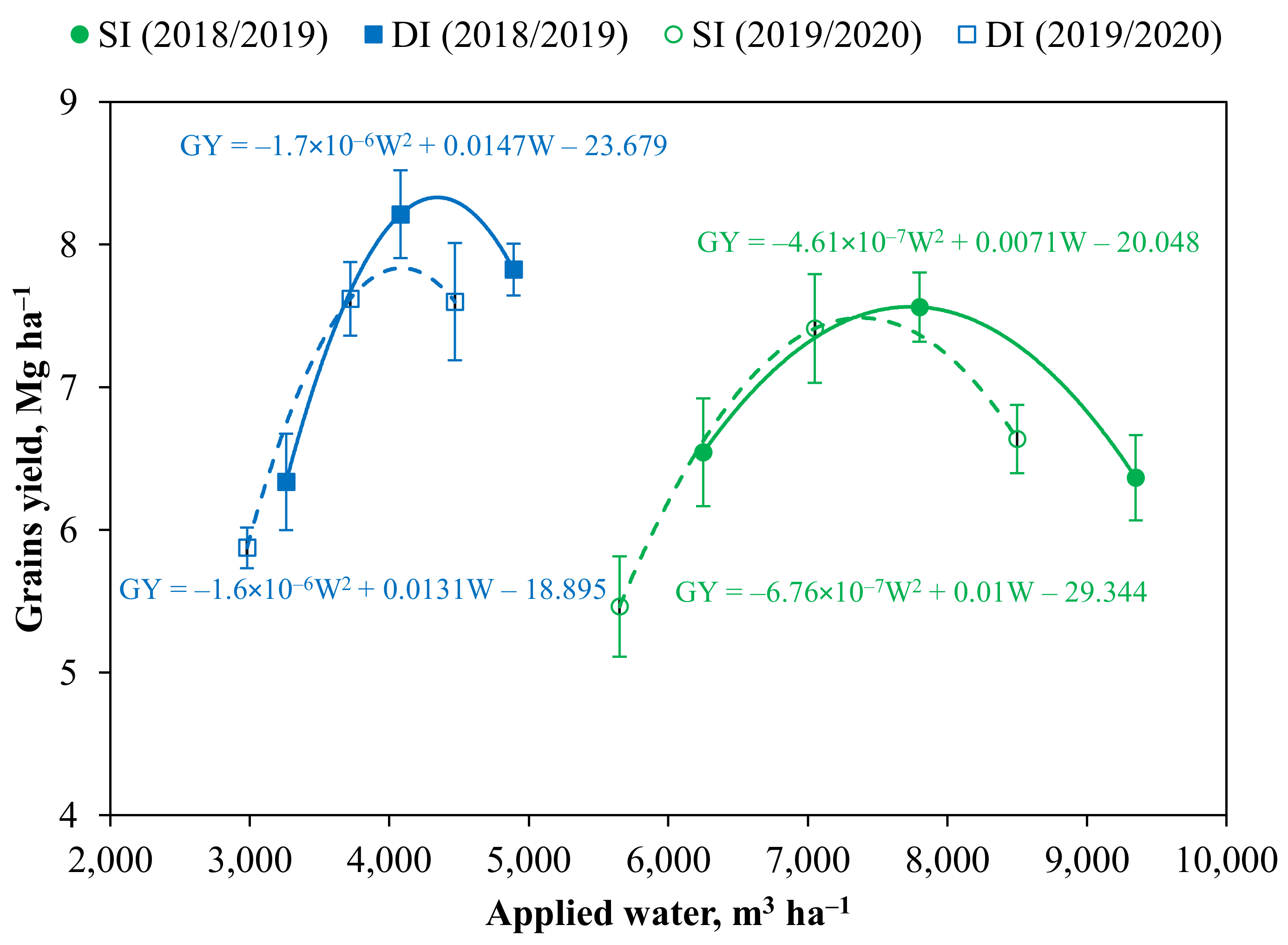
3.3. Grain Yield–Water Relationship
3.4. CROPWAT Model
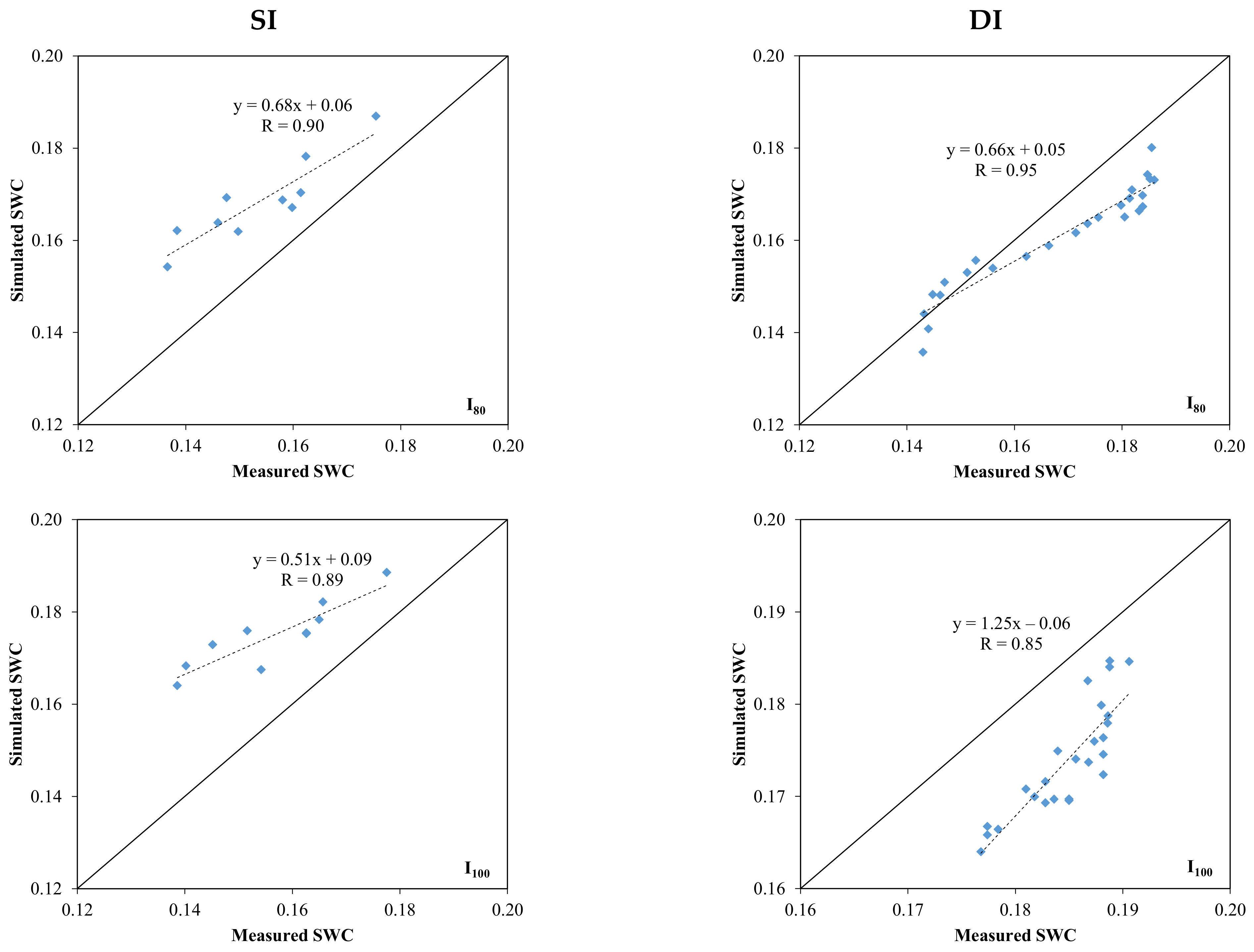
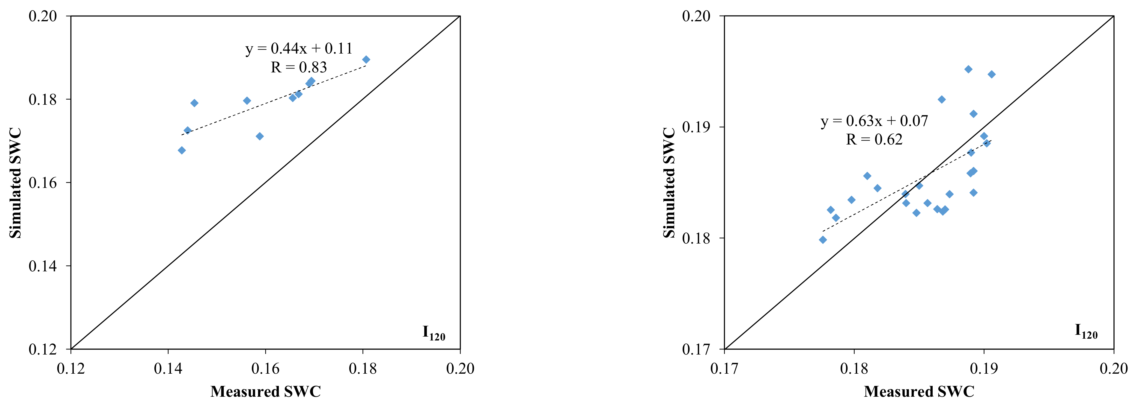
3.5. SALTMED Model
4. Conclusions
Author Contributions
Funding
Institutional Review Board Statement
Informed Consent Statement
Data Availability Statement
Acknowledgments
Conflicts of Interest
References
- Wu, W.; Ma, B.-L. Assessment of canola crop lodging under elevated temperatures for adaptation to climate change. Agric. For. Meteorol. 2018, 248, 329–338. [Google Scholar] [CrossRef]
- Eck, M.; Murray, A.; Ward, A.R.; Konrad, C. Influence of growing season temperature and precipitation anomalies on crop yield in the southeastern United States. Agric. For. Meteorol. 2020, 291, 108053. [Google Scholar] [CrossRef]
- The World Bank. Water in Agriculture. 2020. Available online: https://www.worldbank.org/en/topic/water-in-agriculture (accessed on 12 December 2021).
- Monaghan, J.M.; Daccache, A.; Vickers, L.H.; Hess, T.M.; Weatherhead, E.K.; Grove, I.G.; Knox, J.W. More ‘crop per drop’: Constraints and opportunities for precision irrigation in European agriculture. J. Sci. Food Agric. 2013, 93, 977–980. [Google Scholar] [CrossRef] [PubMed]
- Zhang, T.; Zou, Y.; Kisekka, I.; Biswas, A.; Cai, H. Comparison of different irrigation methods to synergistically improve maize’s yield, water productivity and economic benefits in an arid irrigation area. Agric. Water Manag. 2021, 243, 106497. [Google Scholar] [CrossRef]
- Xu, D.; Li, Y. Review on advancements of study on precision surface irrigation system. J. Hydraul. Eng. 2007, 38, 529–537. [Google Scholar]
- Benjamin, J.G.; Havis, H.R.; Ahuja, L.R.; Alonso, C.V. Leaching and water flow patterns in every-furrow and alternate-furrow irrigation. Soil Sci. Soc. Am. J. 1994, 58, 1511–1517. [Google Scholar] [CrossRef]
- Kang, S.; Liang, Z.; Pan, Y.; Shi, P.; Zhang, J. Alternate furrow irrigation for maize production in an arid area. Agric. Water Manag. 2000, 45, 267–274. [Google Scholar] [CrossRef]
- Amayreh, J.; Al-Abed, N. Developing crop coefficients for field-grown tomato (Lycopersicon esculentum Mill.) under drip irrigation with black plastic mulch. Agric. Water Manag. 2005, 73, 247–254. [Google Scholar] [CrossRef]
- Wang, F.-X.; Wu, X.-X.; Shock, C.C.; Chu, L.-Y.; Gu, X.-X.; Xue, X. Effects of drip irrigation regimes on potato tuber yield and quality under plastic mulch in arid Northwestern China. Field Crops Res. 2011, 122, 78–84. [Google Scholar] [CrossRef]
- Chaves, M.M.; Zarrouk, O.; Francisco, R.; Costa, J.M.; Santos, T.; Regalado, A.P.; Rodrigues, M.L.; Lopes, C.M. Grapevine under deficit irrigation: Hints from physiological and molecular data. Ann. Bot. 2010, 105, 661–676. [Google Scholar] [CrossRef]
- Sezen, S.M.; Yazar, A.; Daşgan, Y.; Yucel, S.; Akyıldız, A.; Tekin, S.; Akhoundnejad, Y. Evaluation of crop water stress index (CWSI) for red pepper with drip and furrow irrigation under varying irrigation regimes. Agric. Water Manag. 2014, 143, 59–70. [Google Scholar] [CrossRef]
- Jovanovic, Z.; Stikic, R. Strategies for Improving Water Productivity and Quality of Agricultural Crops in an Era of Climate Change. In Irrigation Systems and Practices in Challenging Environments; Lee, T.S., Ed.; IntechOpen: Rijeka, Croatia, 2012; pp. 77–102. [Google Scholar]
- Loveys, B.R.; Stoll, M.; Davies, W.J. Physiological approaches to enhance water use efficiency in agriculture: Exploiting plant signaling in novel irrigation practice. In Water Use Efficiency in Plant Biology; Bacon, M.A., Ed.; University of Lancaster: Lancaster, UK, 2004; pp. 113–141. [Google Scholar]
- Yang, H.; Du, T.; Qiu, R.; Chen, J.; Wang, F.; Li, Y.; Wang, C.; Gao, L.; Kang, S. Improved water use efficiency and fruit quality of greenhouse crops under regulated deficit irrigation in northwest China. Agric. Water Manag. 2017, 179, 193–204. [Google Scholar] [CrossRef]
- Chai, Q.; Gan, Y.; Zhao, C.; Xu, H.L.; Waskom, R.M.; Niu, Y.; Siddique, K.H.M. Regulated deficit irrigation for crop production under drought stress. a review. Agron. Sustain. Dev. 2016, 36, 1–21. [Google Scholar] [CrossRef]
- Evett, S.R.; Tolk, J.A. Introduction: Can water use efficiency Be modeled well enough to impact crop management? Agron. J. 2009, 101, 423–425. [Google Scholar] [CrossRef]
- Kato, Y.; Abe, J.; Kamoshita, A.; Yamagishi, J. Genotypic variation in root growth angle in rice (Oryza sativa L.) and its association with deep root development in upland fields with different water regimes. Plant Soil. 2006, 287, 117–129. [Google Scholar] [CrossRef]
- Kirda, C. Deficit irrigation scheduling based on plant growth stages showing water stress tolerance. In Deficit Irrigation Practice; FAO: Rome, Italy, 2002; pp. 3–10. [Google Scholar]
- Stikic, R.; Savic, S.; Jovanovic, Z.; Jacobsen, S.E.; Liu, F.; Jensen, C.R. Deficit irrigation strategies: Use of stress physiology knowledge to increase water use efficiency in tomato and potato. In Horticulture in 21st Century Series: Botanical Research and Practices; Sampson, A.N., Ed.; Nova Science Publishers: New York, NY, USA, 2010; pp. 161–178. [Google Scholar]
- Pequeno, D.N.L.; Hernández-Ochoa, I.M.; Reynolds, M.; Sonder, K.; Moleromilan, A.; Robertson, R.D.; Lopes, M.S.; Xiong, W.; Kropff, M.; Asseng, S. Climate impact and adaptation to heat and drought stress of regional and global wheat production. Environ. Res. Lett. 2021, 16, 054070. [Google Scholar] [CrossRef]
- Khuhro, W.A.; Kandhro, M.N.; Sadiq, N.; Jakhro, M.I.; Amanullah Naseer, N.S.; Latif, S.A. Impact of irrigation stress on agronomic traits of promising wheat varieties in Tandojam-Pakistan. Pure Appl. Biol. 2018, 7, 714–720. [Google Scholar] [CrossRef]
- Meena, R.P.; Tripathi, S.; Sharma, R.; Chhokar, R.; Chander, S.; Jha, A. Role of precision irrigation scheduling and residue-retention practices on water-use efficiency and wheat (Triticum aestivum) yield in north-western plains of India. Indian J. Agron. 2018, 54, 34–47. [Google Scholar]
- Qiu, G.Y.; Wang, L.; He, X.; Zhang, X.; Chen, S.; Chen, J.; Yang, Y. Water use efficiency and evapotranspiration of winter wheat and its response to irrigation regime in the north China plain. Agric. For. Meteorol. 2008, 148, 1848–1859. [Google Scholar] [CrossRef]
- Lobell, D.B.; Ortiz-Monasterio, J.I. Evaluating strategies for improved water use in spring wheat with CERES. Agric. Water Manag. 2006, 84, 249–258. [Google Scholar] [CrossRef]
- Peake, A.S.; Carberry, P.S.; Raine, S.R.; Gett, V.; Smith, R.J. An alternative approach to whole-farm deficit irrigation analysis: Evaluating the risk-efficiency of wheat irrigation strategies in sub-tropical Australia. Agric. Water Manag. 2016, 169, 61–76. [Google Scholar] [CrossRef][Green Version]
- Panda, R.K.; Behera, S.K.; Kashyap, P.S. Effective management of irrigation water for wheat under stressed conditions. Agric. Water Manag. 2003, 63, 37–56. [Google Scholar] [CrossRef]
- Jalota, S.K.; Sood, A.; Chahal, G.B.S.; Choudhury, B.U. Crop water productivity of cotton (Gossypium hirsutum L.)—wheat (Triticum aestivum L.) system as influenced by deficit irrigation, soil texture and precipitation. Agric. Water Manag. 2006, 84, 137–146. [Google Scholar] [CrossRef]
- Wang, Q.; Li, F.; Zhang, E.; Li, G.; Vance, M. The effects of irrigation and nitrogen application rates on yield of spring wheat (longfu-920), and water use efficiency and nitrate nitrogen accumulation in soil. Aust. J. Crop Sci. 2012, 6, 662–672. [Google Scholar]
- Rao, S.S.; Regar, P.L.; Tanwar, S.P.S.; Singh, Y.V. Wheat yield response to line source sprinkler irrigation and soil management practices on medium-textured shallow soils of arid environment. Irrig. Sci. 2013, 31, 1185–1197. [Google Scholar] [CrossRef]
- Gao, Z.; Liang, X.-G.; Lin, S.; Zhao, X.; Zhang, L.; Zhou, L.-L.; Shen, S.; Zhou, S.-L. Supplemental irrigation at tasseling optimizes water and nitrogen distribution for high-yield production in spring maize. Field Crops Res. 2017, 209, 120–128. [Google Scholar] [CrossRef]
- Memon, S.A.; Sheikh, I.A.; Talpur, M.A.; Mangrio, M.A. Impact of deficit irrigation strategies on winter wheat in semi-arid climate of Sindh. Agric. Water Manag. 2021, 243, 106389. [Google Scholar] [CrossRef]
- Sadras, V.O.; Angus, J.F. Benchmarking water-use efficiency of rainfed wheat in dry environments. Aust. J. Agric. Res. 2006, 57, 847–856. [Google Scholar] [CrossRef]
- Ragab, R.; Malash, N.; Abdel Gawad, G.; Arslan, A.; Ghaibeh, A. A Holistic Generic Integrated Approach for Irrigation, Crop and Field Management: 2. The SALTMED Model Validation Using Field Data of Five Growing seasons from Egypt and Syria. Agric. Water Manag. 2005, 78, 89–107. [Google Scholar] [CrossRef]
- Doorenbos, J.; Pruitt, W.O. Guidelines for Predicting Crop Water Requirements, 2nd ed.; FAO Irrigation and Drainage Paper 24; Food and Agriculture Organization of the United Nations: Rome, Italy, 1977; 156p. [Google Scholar]
- Smith, M.; Allen, R.; Monteith, J.; Perrier, L.; Segeren, A. Report on the Expert Consultation for the Revision of FAO Methodologies for Crop Water Requirements; FAO/AGL: Rome, Italy, 1991. [Google Scholar]
- Smith, M. CropWat. In A Computer Program for Irrigation Planning and Management; FAO Irrigation and Drainage Paper 46; Food and Agriculture Organization of the United Nations: Rome, Italy, 1992. [Google Scholar]
- Smith, M. CLIMWAT for CROPWAT, a Climatic Data Base for Irrigation Planning and Management; FAO Irrigation and Drainage Paper 49; Food and Agriculture Organization of the United Nations: Rome, Italy, 1993; 113p. [Google Scholar]
- Allen, R.G.; Pereira, L.S.; Raes, D.; Smith, M. Crop Evapotranspiration: Guidelines for Computing Crop Water Requirements; FAO Irrigation and Drainage Paper 56; FAO: Rome, Italy, 1998. [Google Scholar]
- Doorenbos, J.; Kassam, A. Yield Response to Water; FAO Irrigation and Drainage, Paper 33; FAO, United Nation: Rome, Italy, 1979. [Google Scholar]
- Kuo, S.-F.; Ho, S.-S.; Liu, C.-W. Estimation irrigation water requirements with derived crop coefficients for upland and paddy crops in ChiaNan irrigation association, Taiwan. Agric. Water Manag. 2006, 82, 433–451. [Google Scholar] [CrossRef]
- Elamin, A.W.M.; Saeed, A.B.; Boush, A. Water Use Efficiencies of Gezira, Rahad and New Haifa Irrigated Schemes under Sudan Dryland Condition. Sudan J. Des. Res. 2011, 3, 62–72. [Google Scholar]
- Rajaona, A.; Sutterer, N.; Asch, F. Potential of waste water use for Jatropha cultivation in arid environments. Agriculture 2012, 2, 376–392. [Google Scholar] [CrossRef]
- Garg, K.K.; Wani, S.P.; Rao, A.K. Crop coefficients of Jatropha (Jatropha curcas) and Pongamia (Pongamia pinna ta) using water balance approach. Wiley Interdiscip. Rev. Energy Environ. 2014, 3, 301–309. [Google Scholar]
- Song, L.; Oeumg, C.; Hornbuckle, J. Assessment of rice Water requirement by using CROPWAT model. In Proceedings of the 15th Science Council of Asia Board Meeting and International Symposium, Siem Reap, Cambodia, 15–17 May 2015. [Google Scholar]
- Tsakmakis, I.D.; Zoidou, M.; Gikas, G.D.; Sylaios, G.K. Impact of irrigation technologies and strategies on cotton water footprint using AquaCrop and CROPWAT models. Environ. Process. 2018, 5, 181–199. [Google Scholar] [CrossRef]
- Moseki, O.; Murray-Hudson, M.; Kashe, K. Crop water and irrigation requirements of Jatropha curcas L. in semi-arid conditions of Botswana: Applying the CROPWAT model. Agric. Water Manag. 2019, 225, 105754. [Google Scholar] [CrossRef]
- Ewaid, S.H.; Abed, S.A.; Al-Ansari, N. Water footprint of wheat in Iraq. Water 2019, 11, 535. [Google Scholar] [CrossRef]
- Ragab, R.A. Holistic Generic Integrated Approach for Irrigation, Crop and Field Management: The SALTMED Model. Environ. Model. Softw. 2002, 17, 345–361. [Google Scholar] [CrossRef]
- Ragab, R.; Malash, N.; Abdel Gawad, G.; Arslan, A.; Ghaibeh, A. A Holistic Generic Integrated Approach for Irrigation, Crop and Field Management: 1. The SALTMED Model and Its Calibration Using Field Data from Egypt and Syria. Agric. Water Manag. 2005, 78, 67–88. [Google Scholar] [CrossRef]
- Marwa, M.A.; El-Shafie, A.F.; Dewedar, O.M.; Molina-Martinez, J.M.; Ragab, R. Predicting the water requirement, soil moisture distribution, yield, water yield of peas and impact of climate change using SALTMED model. Plant. Arch. 2020, 20, 3673–3689. [Google Scholar]
- Montenegro, S.G.; Montenegro, A.; Ragab, R. Improving Agricultural Water Management in The Semi-Arid Region of Brazil: Experimental and Modelling Study. Irrig. Sci. 2010, 28, 301–316. [Google Scholar] [CrossRef]
- Mehanna, H.M.; Sabreen, R.H.P.; El-Hagarey, M.E. Validation of SALTMED model under different conditions of drought and fertilizer for snap bean in delta, Egypt. In Proceedings of the Minta International Conference for Agriculture and Irrigation in the Nile Basin Countries, El-Minia, Egypt, 26–29 March 2012. [Google Scholar]
- Pulvento, C.; Riccardi, M.; Lavini, A.; D’andria, R.; Ragab, R. SALTMED Model to Simulate Yield and Dry Matter for Quinoa Crop and Soil Moisture Content under Different Irrigation Strategies in South Italy. Irrig. Drain. 2013, 62, 229–238. [Google Scholar] [CrossRef]
- Rameshwaran, P.; Tepe, A.; Yazar, A.; Ragab, R. The Effect of Saline Irrigation Water on the Yield of Pepper: Experimental and Modeling Study. Irrig. Drain. 2015, 64, 41–49. [Google Scholar] [CrossRef]
- Aly, A.A.; Al-Omran, A.M.; Khasha, A.A. Water management for cucumber: Greenhouse experiment in Saudi Arabia and modeling study using SALTMED model. J. Soil Water Conserv. 2015, 70, 1–11. [Google Scholar] [CrossRef]
- Hassanli, M.; Ebrahimian, H.; Mohammadi, E.; Rahirni, A.; Shokouhi, A. Simulating maize yields when irrigating with saline water, using the AquaCrop, SALTMED, and SWAP models. Agric. Water Manag. 2016, 176, 91–99. [Google Scholar] [CrossRef]
- Al-Omran, A.; Louki, I.; Alkhasha, A.; Abd El-Wahed, M.H.; Obadi, A. Water Saving and Yield of Potatoes under Partial Root-Zone Drying Drip Irrigation Technique: Field and Modelling Study Using SALTMED Model in Saudi Arabia. Agronomy 2020, 10, 1997. [Google Scholar] [CrossRef]
- Page, A.; Miller, R.; Keeney, D. Chemical and microbiological properties. In Methods of Soil Analysis, Part 2, 2nd ed.; Agronomy Monogram 9; Agronomy Society of America and Soil Science Society of America: Madison, WI, USA, 1982. [Google Scholar]
- Klute, A. Methods of Soil Analysis; Part 1 Book Series No. 9; American Society of Agronomy and Soil Science America: Madison, WI, USA, 1986. [Google Scholar]
- Jarvan, M.; Edesi, L.; Adamson, A. Effect of sulphur fertilization on grain yield and yield components of winter wheat. Acta Agric. Scand. 2012, 62, 401–409. [Google Scholar] [CrossRef]
- Xie, Y.; Zhang, H.; Zhu, Y.; Zhao, L.; Yang, J.; Cha, F.; Liu, C.; Wang, C.; Guo, T. Grain yield and water use of winter wheat as affected by water and sulfur supply in the North China Plain. J. Integr. Agric. 2017, 16, 614–625. [Google Scholar] [CrossRef]
- Kijne, J.; Barker, R.; Molden, D. Improving water productivity in agriculture. In Water Productivity in Agriculture: Limits and Opportunities for Improvement; Kijne, J., Barker, R., Eds.; International Water Management Institute: Colombo, Sri Lanka, 2003; pp. 11–19. [Google Scholar]
- Helweg, O. Functions of crop yield from applied water. Agron. J. 1991, 83, 769–773. [Google Scholar] [CrossRef]
- Swennenhuis, J. CROPWAT Version 8.0 Model; FAO, Viale delle Terme di Caracalla: Rome, Italy, 2009; Available online: http://www.fao.org/nr/water/infores_databases_cropwat.html (accessed on 12 January 2022).
- Van Genuchten, M.T. A closed-form equation for predicting the hydraulic conductivity of unsaturated soils. Soil Sci. Soc. Am. J. 1980, 44, 892–898. [Google Scholar] [CrossRef]
- Legates, D.R.; McCabe, G.J., Jr. Evaluating the use of “goodness-of fit” measures in hydrologic and hydroclimatic model validation. Water Resour. Res. 1999, 35, 233–241. [Google Scholar] [CrossRef]
- Willmott, C.J.; Matsuura, K. Advantages of the mean absolute error (MAE) over the root mean square error (RMSE) in assessing average model performance. Clim. Res. 2005, 30, 79–82. [Google Scholar] [CrossRef]
- CoStat Version 6.303 Copyright 1998–2004 CoHort Software798 Lighthouse Ave. PMB 320, Monterey, CA, 93940, USA. Available online: https://cohortsoftware.com/costat.html (accessed on 2 October 2021).
- Snedecor, G.; Cochran, W. Statistical Method, 7th ed.; Ames, I.A., Ed.; The Iowa State University Press: Ames, IA, USA, 1980. [Google Scholar]
- Moussa, A.M.; Abdel-Maksoud, H.H. Effect of soil moisture regime on yield and its components and water use efficiency for some wheat cultivars. Ann. Agric. Sci. 2004, 49, 515–530. [Google Scholar]
- Abdelkhalek, A.A.; Darwesh, R.K.; El-Mansoury, M.A.M. Response of some wheat varieties to irrigation and nitrogen fertilization using ammonia gas in North Nile Delta region. Ann. Agric. Sci. 2015, 60, 245–256. [Google Scholar] [CrossRef]
- Pandey, D.S.; Kumar, D.; Misra, R.D.; Prakash, A.; Gupta, V.K. An integrated approach of irrigation and fertilizer management to reduce lodging in wheat (Triticum aestivum). Indian J. Agron. 1997, 42, 86–89. [Google Scholar]
- Eissa, M.A. Improving Yield of Drip-Irrigated Wheat under Sandy Calcareous Soils. World Appl. Sci. J. 2014, 30, 818–826. [Google Scholar]
- Noreldin, T.; Ouda, S.; Mounzer, O.; Abdelhamid, M.T. CropSyst model for wheat under deficit irrigation using sprinkler and drip irrigation in sandy soil. J. Water Land Dev. 2015, 26, 57–64. [Google Scholar] [CrossRef]
- Mugabe, F.T.; Nyakatawa, E.Z. Effect of deficit irrigation on wheat and opportunities of growing wheat on residual soil moisture in southeast Zimbabwe. Agric. Water Manag. 2000, 46, 111–119. [Google Scholar] [CrossRef]
- Ali, M.H.; Hoque, M.R.; Hassan, A.A.; Khair, A. Effects of deficit irrigation on yield, water productivity, and economic returns of wheat. Agric. Water Manag. 2017, 92, 151–161. [Google Scholar] [CrossRef]
- Geerts, S.; Raes, D. Deficit irrigation as an on-farm strategy to maximize crop water productivity in dry areas. Agric. Water Manag. 2009, 96, 1275–1284. [Google Scholar] [CrossRef]
- Pereira, L.S.; Oweis, T.; Zairi, A. Irrigation management under water scarcity. Agric. Water Manag. 2002, 57, 175–206. [Google Scholar] [CrossRef]
- Maurya, R.K.; Singh, G.R. Effect of crop establishment methods and irrigation schedules on economics of wheat (Triticum aestivum) production moisture depletion pattern, consumptive use and crop water use efficiency. Indian J. Agric. Sci. 2008, 78, 830–833. [Google Scholar]
- Knežević, M.; Perović, N.; Životić, L.; Ivanov, M.; Topalović, A. Simulation of winter wheat water balance with CROPWAT and ISAREG models. Agric. For. 2013, 59, 41–53. [Google Scholar]
- Zhou, H.; Zhao, W. Modeling soil water balance and irrigation strategies in a flood-irrigated wheat-maize rotation system. A case in dry climate, China. Agric. Water Manag. 2019, 221, 286–302. [Google Scholar] [CrossRef]
- English, M. Deficit irrigation. I: Analytical framework. J. lrrig. Drain. Eng. 1990, 116, 399–412. [Google Scholar] [CrossRef]
- Fereres, E.; Garda-Vila, M. Irrigation Management for Efficient Crop Production. In Crop Science; Savin, R., Slafer, G.A., Eds.; Springer: New York, NY, USA, 2019; pp. 345–360. [Google Scholar]
- Bennett, D.R.; Harms, T.E. Crop yield and water requirement relationships for major irrigated crops in southern Alberta. Can. Water Resour. J. 2011, 36, 159–170. [Google Scholar] [CrossRef]
- Karandisha, F.; Simunek, J. A comparison of the HYDRUS (2D/3D) and SALTMED models to investigate the influence of various water-saving irrigation strategies on the maize water footprint. Agric. Water Manag. 2019, 213, 809–820. [Google Scholar] [CrossRef]
- Hirich, A.; Ragab, R.; Choukr-Allah, R.; Rami, A. The effect of deficit irrigation with treated wastewater on sweet corn: Experimental and modelling study using SALTMED model. Irrig Sci. 2014, 32, 205–219. [Google Scholar] [CrossRef]
- Kaya, C.I.; Yazar, A.; Sezen, S. SALTMED model performance on simulation of soil moisture and crop yield for quinoa irrigated using different irrigation systems, 1rn·galion strategies and water qualities in Turkey. Agric. Agric. Sci. Procedia 2015, 4, 108–118. [Google Scholar]
- Hirich, A.; Choukr-Allah, R.; Ragab, R.; Jacobsen, S.-E.; El Youssfi, L.; El-Omari, H. The SALTMED model calibration and validation using field data from Morocco. J. Mater Environ. Sci. 2012, 3, 342–359. [Google Scholar]


| Soil’s Physical Properties | |||||||||||
|---|---|---|---|---|---|---|---|---|---|---|---|
| Depth (cm) | Particle Size (%) | Texture | ρb (g cm−3) | FC (%) | WP (%) | θs m3 m−3 | TAW m3 m−3 | Ks (mm h−1) | |||
| Sand | Silt | Clay | |||||||||
| 0–30 | 72.1 | 11.9 | 16.0 | Loamy sand | 1.57 | 20.0 | 12.0 | 0.44 | 0.08 | 32.5 | |
| 30–60 | 73.4 | 12.0 | 14.6 | Loamy sand | 1.51 | 19.5 | 11.5 | 0.43 | 0.08 | 33.1 | |
| Soil’s Chemical Properties | |||||||||||
| Depth (cm) | ECe (dS m−1) | pH | OM | Soluble Cations (meq L−1) | Soluble Anions (meq L−1) | ||||||
| Ca2+ | Mg2+ | Na+ | K+ | CO32− | HCO3− | SO42− | Cl− | ||||
| 0–30 | 4.42 | 7.87 | 0.7 | 28.7 | 7.74 | 9.62 | 0.46 | - | 2.98 | 22.00 | 21.56 |
| 30–60 | 5.56 | 7.74 | 0.8 | 27.8 | 5.88 | 18.88 | 0.35 | - | 2.97 | 22.98 | 23.93 |
| Treatments | Plant Height | Number of Spikes | Spike Length | 1000-Kernel Weight | Biological Yield | Grain Yield | Harvest Index | ||||||||
|---|---|---|---|---|---|---|---|---|---|---|---|---|---|---|---|
| df | p-Value | LSD | p-Value | LSD | p-Value | LSD | p-Value | LSD | p-Value | LSD | p-Value | LSD | p-Value | LSD | |
| 2018/2019 | |||||||||||||||
| Irr. syst. | 1 | 0.1417 | ns | 0.2680 | ns | 0.3037 | ns | 0.1063 | ns | 0.0747 | ns | 0.0188 | 0.51 | 0.4502 | ns |
| Irr. lev. | 2 | 0.9522 | ns | 0.4414 | ns | 0.1998 | ns | <0.001 | 1.58 | 0.0239 | 1.48 | 0.0008 | 0.63 | 0.1491 | ns |
| Irr. syst. × Irr. lev. | 2 | 0.2830 | ns | 0.4651 | ns | 0.9103 | ns | 0.3825 | ns | 0.2375 | ns | 0.0405 | 0.89 | 0.1187 | ns |
| CV, % | 3.78 | 19.44 | 6.05 | 3.53 | 8.17 | 8.26 | 6.86 | ||||||||
| 2019/2020 | |||||||||||||||
| Irr. syst. | 1 | 0.4590 | ns | 0.2852 | ns | 0.9403 | ns | 0.2042 | ns | 0.0919 | ns | 0.0476 | 0.52 | 0.2376 | ns |
| Irr. lev. | 2 | 0.3757 | ns | <0.001 | 21.99 | 0.3518 | ns | 0.0022 | 3.93 | <0.001 | 0.57 | <0.001 | 0.64 | 0.0853 | ns |
| Irr. syst. × Irr. lev. | 2 | 0.0829 | ns | 0.5231 | ns | 0.4794 | ns | 0.5828 | ns | 0.3245 | ns | 0.4472 | ns | 0.3028 | ns |
| CV, % | 2.74 | 5.63 | 6.91 | 8.57 | 3.29 | 8.85 | 10.83 | ||||||||
| Irrigation Systems | Irrigation Levels | 2018/2019 | 2019/2020 | ||||
|---|---|---|---|---|---|---|---|
| RMSE | MAE | MARE, % | RMSE | MAE | MARE, % | ||
| SI | I80 | 0.019 | 0.016 | 9.0 | 0.018 | 0.015 | 8.5 |
| I100 | 0.022 | 0.02 | 11.5 | 0.020 | 0.018 | 9.9 | |
| I120 | 0.022 | 0.02 | 11.4 | 0.021 | 0.019 | 10.3 | |
| DI | I80 | 0.018 | 0.015 | 9.7 | 0.017 | 0.013 | 8.8 |
| I100 | 0.016 | 0.011 | 6.6 | 0.023 | 0.018 | 11.3 | |
| I120 | 0.015 | 0.009 | 5.3 | 0.017 | 0.010 | 6.0 | |
| Growing Season | Treatments | Biological Yield | RE (%) | Grain Yield | RE (%) | |||
|---|---|---|---|---|---|---|---|---|
| Irrigation Systems | Irrigation Levels | Observed | Simulated | Observed | Simulated | |||
| 2018/2019 | SI | I80 | 15.75 | 18.20 | 15.54 | 6.54 | 7.55 | 15.47 |
| I100 | 18.00 | 17.98 | −0.11 | 7.56 | 7.57 | 0.13 | ||
| I120 | 15.50 | 18.37 | 18.54 | 6.36 | 7.58 | 19.18 | ||
| DI | I80 | 16.25 | 20.21 | 24.37 | 6.34 | 7.54 | 18.95 | |
| I100 | 18.25 | 18.37 | 0.65 | 8.21 | 8.27 | 0.68 | ||
| I120 | 18.00 | 19.04 | 5.80 | 7.83 | 8.28 | 5.80 | ||
| RMSE | 2.27 | 0.83 | ||||||
| MAE | 1.74 | 0.66 | ||||||
| MARE, % | 10.80 | 10.04 | ||||||
| 2019/2020 | SI | I80 | 14.45 | 18.22 | 26.09 | 5.46 | 6.85 | 25.41 |
| I100 | 16.88 | 17.98 | 6.52 | 7.41 | 7.56 | 2.02 | ||
| I120 | 16.93 | 18.37 | 8.53 | 6.64 | 7.57 | 14.01 | ||
| DI | I80 | 15.11 | 19.61 | 29.81 | 5.88 | 7.14 | 21.51 | |
| I100 | 17.49 | 18.16 | 3.80 | 7.62 | 8.17 | 7.22 | ||
| I120 | 16.84 | 18.95 | 12.55 | 7.60 | 8.24 | 8.48 | ||
| RMSE | 2.67 | 0.92 | ||||||
| MAE | 2.27 | 0.82 | ||||||
| MARE, % | 14.55 | 13.11 | ||||||
Publisher’s Note: MDPI stays neutral with regard to jurisdictional claims in published maps and institutional affiliations. |
© 2022 by the authors. Licensee MDPI, Basel, Switzerland. This article is an open access article distributed under the terms and conditions of the Creative Commons Attribution (CC BY) license (https://creativecommons.org/licenses/by/4.0/).
Share and Cite
El-Shafei, A.A.; Mattar, M.A. Irrigation Scheduling and Production of Wheat with Different Water Quantities in Surface and Drip Irrigation: Field Experiments and Modelling Using CROPWAT and SALTMED. Agronomy 2022, 12, 1488. https://doi.org/10.3390/agronomy12071488
El-Shafei AA, Mattar MA. Irrigation Scheduling and Production of Wheat with Different Water Quantities in Surface and Drip Irrigation: Field Experiments and Modelling Using CROPWAT and SALTMED. Agronomy. 2022; 12(7):1488. https://doi.org/10.3390/agronomy12071488
Chicago/Turabian StyleEl-Shafei, Ahmed A., and Mohamed A. Mattar. 2022. "Irrigation Scheduling and Production of Wheat with Different Water Quantities in Surface and Drip Irrigation: Field Experiments and Modelling Using CROPWAT and SALTMED" Agronomy 12, no. 7: 1488. https://doi.org/10.3390/agronomy12071488
APA StyleEl-Shafei, A. A., & Mattar, M. A. (2022). Irrigation Scheduling and Production of Wheat with Different Water Quantities in Surface and Drip Irrigation: Field Experiments and Modelling Using CROPWAT and SALTMED. Agronomy, 12(7), 1488. https://doi.org/10.3390/agronomy12071488