Optimum Plant Density for Increased Groundnut Pod Yield and Economic Benefits in the Semi-Arid Tropics of West Africa

Abstract

Groundnut is a very important crop in the West and Central Africa (WCA) region, accounting for almost 70% of Africa’s groundnut production in 2019. Despite its economic importance, the crop’s yield is still low. For a high yield and profitable economic returns, optimal plant density is a fundamental crop management practice. Plant density experiments were conducted at the ICRISAT-Mali research station between 2016 and 2021 over the main rainy and dry seasons to determine the optimum density for maximum groundnut yield and economic benefits. The treatments contained row spacing of 20 cm, 30 cm, 40 cm, 50 cm, 60 cm, 70 cm, 80 cm, 90 cm, and 100 cm, with intra-row spacing of 10 cm, 15 cm, and 20 cm. Results showed that when plant density was increased, dry pod yield, production value, and net economic benefit per hectare increased in a no moisture stress scenario. During the rainy season, the 40 cm × 10 cm spacing gave the highest dry pod yield (1693 kg), production value ($891.6), and net benefit ($403.5) per hectare. The highest dry pod yield (3703 kg), production value ($2173), and net benefit ($1510.2) per hectare were obtained from 30 cm × 10 cm spacing during the dry season. The number of pods per plant and 100 SW increased with lower plant densities. Therefore, it is recommended to increase plant density to at least 222,000 plants per hectare in the Sudan Savannah agroecology of WCA.

1. Introduction

Groundnut (Arachis hypogaea L.), also known as peanut, is an important crop for smallholder farmers in Africa, as it provides both food and cash income. In 2019, Africa accounted for 57% of the 29.6 million hectares of global groundnut area and 34% of the 48 million tonnes of global groundnut production [1]. West and Central Africa (WCA) accounted for more than 64% of the continent’s area under groundnut and 70% of groundnut production. Nigeria remained the largest producer in WCA and Africa, with 3.9 million hectares and 4.5 million tonnes produced, followed by Senegal with 1.1 million hectares and 1.4 million tonnes produced. Groundnut is a nutrient-dense crop with 22–30% protein, 35–60% oil, and a wide range of minerals, vitamins, and bioactive substances. The grain is consumed in various forms by smallholder farmers, including fresh, roasted, boiled, paste (butter), oil, and sauces [2], and the butter or crushed grain is commonly used in the preparation of local foods such as ‘Baag-benda’ (groundnut sauce with vegetables), ‘tigadegena’ (groundnut stew), and Kuli kuli (groundnut cake—crispy snack often made from a byproduct of groundnut oil extraction). Groundnut is also known for its suitability for creating ready-to-use therapeutic foods (RUTF) such as Plumpy’Nut (peanut butter paste fortified with milk and vitamins) to treat malnutrition in vulnerable groups such as pregnant and lactating women, as well as children under the age of two [3,4]. It provides an important source of animal feed as a form of haulms and groundnut cake. Groundnut is also chosen for crop rotation since it has the potential to fix atmospheric nitrogen, which benefits the following crop. As a cash crop, it is widely marketed accounting for up to 50% or more of rural household cash income [5,6]. The traded groundnut is either used for home consumption or further processed for oil extraction. Groundnut is often referred to as a “women’s crop” in WCA and it employs a high number of women and youth in the cultivation, processing, and marketing, hence fostering their economic participation and empowerment [2,6]. In some countries, such as Nigeria, women are in charge of practically all small-scale groundnut oil processing. Despite its importance, groundnut productivity in WCA is low, at roughly 1 tonne per hectare, compared with the global average of 1.65 tonnes and industrialized countries such as the United States, which have more than 3.5 tonnes [1]. This is due to various production constraints including moisture stress, use of low-yielding obsolete varieties, diseases (e.g., early leaf spot, rosette) and poor crop management practices among others. Hence, groundnut productivity in the region must be increased by utilizing improved cultivars and crop management approaches.

Optimum plant density (spacing between plants) is among the critical crop management practices for obtaining a high groundnut yield and profitable economic returns. Various authors have indicated that maximum or optimum yields of groundnut were obtained with higher plant densities, e.g., [7,8,9,10,11]. In India, the optimum population of 330,000 plants per hectare (30 cm × 10 cm) for Spanish/Valencia cultivars and 148,000 plants per hectare (45 cm × 15 cm) for Virginia cultivars were reported [7]. In Africa, different spacings between rows and plants within a row are used by national breeding and extension programs, especially those in West Africa. For example, for Sudanian agroecology in Nigeria, spacing of 75 cm × 10 cm with two seeds sown per hill (266,667 plants per hectare) was recommended [11], while spacings of 75 cm × 20 cm (133,333 plants per hectare); 75 cm × 10 cm (266,667 plants per hectare), or 50 cm × 20 cm (200,000 plants per hectare) for bunch varieties, and 75 cm × 20 cm (133,333 plants per hectare) or 75 cm × 25 cm (106,667 plants per hectare) for semi-spreading and spreading varieties were recently suggested for North-East Nigeria [12], where two seeds should be sown per hill at 5 cm depth. The Institute of Agricultural Research (IAR), which is the national coordinating institute for groundnut research in Nigeria, utilizes 75 cm inter-row and 20 cm intra-row spacing with two seeds per hill [13], which gives 133,333 plants per hectare. The Mali variety release and registration guideline requires 40 cm × 15 cm (166,667 plants per hectare) for short duration (90 days maturity) erect/bunch varieties and 60 cm × 15 cm (111,111 plants per hectare) for long duration (90–120 days) varieties for Distinction, Homogénéité, Stabilité (DHS), and Valeur Agronomique et Technologique (VAT) field evaluations [14]. In Ghana, Oteng-Frimpong et al. [15] indicated a recommended spacing of 40 cm × 15 cm (166,667 plants per hectare) for erect or semi-erect varieties and 50 cm × 20 cm (100,000 plants per hectare) for spreading varieties with one seed per hill unless the germination rate is between 70 and 84%, in which case two seeds are sown per hill. Recently, the optimal spacing for groundnut in smallholder farming systems in Ghana’s Upper West, Upper East, and Northern Regions was reported to be 30 cm × 15 cm, i.e., 220,000 plants per hectare [16]. In the ICRISAT-WCA groundnut breeding program, the spacing between rows (inter-row) and plants within a row (intra-row) is 60 cm and 10 cm, respectively, i.e., 166,667 plants per hectare. Stakeholders who participated in participatory variety selection and field and exchange visits at the ICRISAT station or on-farm fields, on the other hand, often wondered about the need to increase density in order to boost yield. Furthermore, based on the results of crop simulation models, a significant increase in plant density for Spanish types to 400,000 plants per hectare was proposed to boost groundnut yield in WCA [17]. With this background, a plant density experiment was conducted between 2016 and 2021 during the main rainy and dry seasons with the objective of maximizing groundnut yield and economic benefits by establishing the optimum plant spacing.

2. Materials and Methods

2.1. Experimental Site

The experiment was carried out during both the rainy (main) and dry (off) seasons. From 2016 to 2018, the rainy season experiment lasted three years, while the dry season experiment lasted two years, from 2020 to 2021. Both experiments were carried out at the International Crops Research Institute for the Semi-Arid Tropics in Mali (ICRISAT-Mali), Samanko station experimental field. With geographic coordinates of 12°5′ N, 8°54′ W, Samanko station lies 26 km southwest of Bamako. The station is located in the Sudan Savannah zone, and the rainy season lasts from June to October. The yearly rainfall is between 800 and 1200 mm. The soil is characteristic of Sudan agroecology referred to as red ferruginous tropical soils (‘sols ferrugineux tropicaux lessives modaux a facies rouge’ in French), an Alfisol consisting primarily of sandy-clay soil with a pH of 4.5, low fertility, and low organic matter content.

Table 1. Meteorological data during the experiment period.

Season	Total Rainfall (mm)			Relative Humidity			Temperature (°C)
Rainy	2016	2017	2018	2016	2017	2018	2016		2017		2018
							min	max	min	max	min	max
July	457.7	398.3	252.3	76.7	77.7	71.7	21.9	31.9	21.7	32.7	22.7	34.8
August	471.0	402.1	359.6	76.9	76.6	74.8	21.6	31.7	21.9	32.1	22.6	34.6
September	170.0	217.4	255.3	70.1	74.2	75.5	21.8	33.4	21.5	33.8	22.9	34.9
October	25.9	0	39.8	71.4	63.1	74.7	21.5	36.6	20.8	36.0	23.0	36.1
Dry	2020	2021		2020	2021		2020		2021
January	0	0		58.3	36.7		15.4	36.6	17.4	38.6
February	0	0		49.0	38.9		18	40.1	19.3	38.9
March	0	0		47.4	45.1		20.6	41.9	25.0	41.0
April	11.9	30.7		46.2	43.1		25.5	44.2	25.5	44.6

shows the meteorological data of the station during the experiment period. Before planting, the experiment site was plowed and disc harrowed by a tractor, with DAP fertilizer applied at a rate of 100 kg/ha. The Niger River runs alongside the station, providing irrigation during the dry season. The RN5 highway divides the experiment station. The main (rainy) season experiment was carried out on the opposite side of the road, dubbed the ‘Cabane,’ and was rainfed with no supplementary irrigation. During the three years of the rainy season experiment, Figure 1 depicts the rainfall distribution in September and October in a cluster of five days. The two months are the critical months for the groundnut grain filling process. There was no rain after mid-September in 2017 and the experimental site received the last rain on 5 September. The dry season experiment was carried out on the Niger riverside of the RN5 highway, with sprinkler irrigation fed from the river. For the first month, the plots were irrigated every other day, then twice a week for the remainder of the crop’s growing cycle.

2.2. Treatments

There were 25 treatments in total, arranged in a randomized complete block design with three replications, with 9 between row (inter-row) and 3 between plant (intra-row) spacings considered (

Table 2. Spacing (between rows and plants within a row), and production cost for rainy and dry seasons.

Treatment Number	Spacing between Rows (cm)	Spacing between Plants in a Row (cm)	Density (Plants/ha)	Production Cost ($)
				Rainy Season	Dry Season
1	20	10	500,000	789	863
2	30	10	333,333	581	662
3	40	10	250,000	487	569
4	50	10	200,000	427	509
5	60	10	166,667	392	473
6	70	10	142,857	364	445
7	80	10	125,000	339	421
8	90	10	111,111	317	398
9	100	10	100,000	309	391
10	20	15	333,333	675	756
11	30	15	222,222	509	591
12	40	15	166,667	432	514
13	50	15	133,333	385	467
14	60	15	111,111	357	438
15	70	15	95,238	333	414
16	80	15	83,333	312	393
17	90	15	74,074	289	370
18	20	20	250,000	622	703
19	30	20	166,667	473	554
20	40	20	125,000	407	488
21	50	20	100,000	363	444
22	60	20	83,333	339	420
23	70	20	71,429	318	399
24	80	20	62,500	299	380
25	90	20	55,556	280	361

). The inter-row spacing of 100 cm was paired with the 10 cm intra-row spacing only, not the 15 cm and 20 cm intra-row spacings. This is because the latter combinations would result in plant densities that were too low for the test to be meaningful. The experiment used an improved groundnut variety, ICGV 86124, which is a Spanish type with a bunch growth habit, early maturity (85–95 days), and drought tolerance. To protect seeds and seedlings from early season insect pests and soilborne diseases, the seed was treated with Apron Star 42 WS (2.5 g per kg) at planting. The plot was 4 m long and 4 m wide. According to the treatments, the number of rows and plants in a plot varied, resulting in a different number of plants per hectare. The treatment with the widest inter-row spacing (100 cm) had 4 rows, whereas the treatment with the narrowest row spacing (20 cm) had 20 rows. Table 2 shows the number of plants per hectare for each treatment. Plots were weeded twice after planting, at 45 and 60 days. At 45 days after planting, 400 kg of gypsum was applied per hectare

2.3. Data Collection and Analysis

Data was collected on the number of matured pods per plant (average of five plants)—NMP, dry weight of pods per plot (DPY, kg/plot), dry weight of haulms per plot (DHY, kg/plot), shelling percent (%) from 200 random pods, and dry weight of 100 seeds (100 SW). For statistical analysis, the DPY and DHY were transformed to per hectare values by multiplying the plot level value (in kg) by 10,000 (m²) and dividing by plot size (m²). The difference between treatments for DPY, DHY, NMP, 100 SW, and shelling percent was tested using an analysis of variance (ANOVA) using Genstat v.20, Hemel Hempstead, England, UK. The F-test was employed to compare treatments with the ANOVA null hypothesis of equal means using Fisher’s protected LSD test.

In addition, data on groundnut grain and haulm production costs and prices were gathered for benefit-to-cost analysis. Certified seed, seed treatment with Apron Star 42 WS, plowing, row preparation and planting, first and second weeding, gypsum, diammonium phosphate (DAP), and harvesting were all included in the production cost. The cost of irrigation was added for the dry season. Labor costs for planting and harvesting were assumed variable depending on the number of rows and plants per hectare, unlike Ajeigbe et al. [11] who assumed constant cost across plant density. During the rainy season, the cost of producing groundnut on one hectare ranged from USD 280 for 90 cm × 20 cm spacing to USD 789 for 20 cm × 10 cm spacing, while during the dry season, it ranged from USD 361 for 90 cm × 20 cm spacing to USD 863 for 20 cm × 10 cm spacing, with seed and labor costs accounting for a significant portion of the cost of higher plant densities (Table 2). Family labor, which is often unpaid, was not taken into account, even though smallholder farmers rely on family labor for much of their fieldwork while purchasing inputs. The net benefit for each treatment was computed by subtracting the production cost from the total production value. Then, by dividing the net benefit by the production cost, the benefit-to-cost ratio (or the net benefit from each unit cost) was established. The total product value, net benefit, and benefit-to-cost ratio were subjected to ANOVA to compare treatments based on the mean of the estimates for each treatment per year, type of season (rainy, dry), and across years and seasons. The estimations were performed using GenStat Ver. 20, Hemel Hempstead, England, UK.

3. Results

3.1. Effect of Plant Density on Yield and Yield Components for Each Year

During the rainy season, the ANOVA results for dry pod yield (DPY) in 2016, 2017, and 2018 revealed a highly significant difference (p < 0.001) between treatments (

Table 3. Mean performance of spacing treatments for DPY, DHY, NMP, 100 SW, and shelling % during the rainy season in 2016, 2017, and 2018.

Spacing (cm) Inter × Intra Row	DPY (kg/ha)			DHY (kg/ha)			NMP			100 SW (g)			Shelling %
	2016	2017	2018	2016	2017	2018	2016	2017	2018	2016	2017	2018	2016	2017	2018
20 × 10	1301	912	1734	798.6	935	817	22.1	24.3	24.7	30.3	24.3	26.3	68.3	61.7	62.0
30 × 10	1283	763	1841	853.5	848	848	22.7	25.3	23.3	27.0	26.3	26.7	70.3	61.7	62.7
40 × 10	1568	625	1818	997.4	1130	1120	25.0	22.7	23.3	33.7	30.7	27.1	64.8	61.0	62.0
50 × 10	1136	900	1825	1025	1108	1064	22.7	24.7	22.7	25.0	35.0	32.7	61.4	62.0	62.2
60 × 10	1269	1019	1272	1059	1019	1239	21.7	24.7	25.2	25.3	27.3	27.3	66.7	62.0	60.7
70 × 10	1196	1006	1485	725.1	1176	1199	20.6	25.3	23.3	32.7	28.7	26.3	61.0	62.0	62.3
80 × 10	1125	1451	1139	1114.6	1330	1479	24.0	24.7	23.3	37.3	38.5	32.0	68.9	62.3	62.7
90 × 10	1292	1366	1083	1118.7	1583	1392	22.3	25.3	23.3	21.2	34.5	28.7	68.0	61.0	61.0
100 × 10	1040	1442	1021	1166.2	1368	1492	24.0	26.0	25.3	29.0	25.3	24.7	65.8	62.0	63.0
20 × 15	1315	1051	1956	807.9	1134	884	24.7	24.0	23.3	30.0	32.7	33.3	65.8	62.7	61.5
30 × 15	1194	699	1939	868.7	1008	859	24.6	24.0	26.0	26.7	30.0	29.3	66.2	61.5	62.5
40 × 15	1196	766	1451	718.1	1005	1047	20.3	24.0	24.7	34.0	24.7	26.7	68.8	61.8	62.2
50 × 15	1000	1197	1690	770.6	1092	1069	21.3	24.7	24.0	33.7	34.3	34.3	69.0	61.7	62.7
60 × 15	1144	444	1453	977.8	1108	947	20.5	22.7	24.7	33.0	28.3	28.0	67.8	61.5	62.5
70 × 15	1063	893	1381	952.4	1429	1229	23.7	22.7	25.3	32.7	35.7	36.7	67.8	61.0	62.0
80 × 15	1035	1153	875	1270.8	1493	1122	21.3	24.0	24.0	30.7	28.7	27.0	63.2	61.0	61.3
90 × 15	545	1961	963	1424.5	1530	1635	22.0	23.3	25.1	36.7	41.0	41.1	64.7	62.5	62.7
20 × 20	1363	787	1984	932.9	912	803	21.7	24.0	24.0	28.3	33.3	33.7	67.2	63.2	63.5
30 × 20	836	575	1005	729.8	1136	765	20.8	25.3	24.0	24.0	26.3	27.3	66.7	62.3	62.7
40 × 20	1193	690	1276	994.8	1161	904	23.0	24.7	23.7	29.7	35.0	32.0	64.3	61.3	62.3
50 × 20	881	811	1378	833.3	1222	500	22.3	24.0	24.7	31.3	30.3	30.0	69.2	61.2	62.3
60 × 20	839	1017	1228	1033.3	1253	916	24.7	25.3	24.3	28.0	29.3	29.3	63.0	61.5	62.5
70 × 20	839	1369	1054	993	1244	848	22.3	24.0	26.0	30.7	32.3	32.0	61.6	62.8	64.2
80 × 20	878	1728	1076	1637.3	1424	972	23.0	24.7	25.3	40.0	32.7	31.3	65.8	63.5	62.7
90 × 20	847	1134	1113	1053.1	1614	1537	20.4	24.7	25.3	33.0	37.0	35.3	64.2	62.3	61.2
Mean	1095	1030	1402	994	1211	1068	22.5	24.4	24.4	30.6	31.3	30.4	66.0	61.9	62.3
Probability	<0.001	<0.001	<0.001	<0.05	<0.001	<0.001	ns	ns	<0.01	0.026	0.004	0.002	0.004	ns	ns
LSD	319.4	454.4	403.9	262.5	297	337.1	3.113	2.082	1.718	8.903	8.059	6.819	4.738	2.523	1.905
CV (%)	17.7	26.8	17.5	16	14.9	19.2	8.4	5.2	4.3	17.7	15.7	13.7	4.4	2.5	1.9

DPY = dry pod yield; DHY = dry haulm yield; NMP = number of matured pods; 100 SW = hundred seed weight; LSD = least significant difference; ns = non-significant; CV = coefficient of variation.

). In 2016, the DPY ranged from 545 kg/ha for 90 cm × 15 cm spacing to 1568 kg/ha for 40 cm × 10 cm spacing (mean = 1095 kg/ha), and from 444 kg/ha for 60 cm × 15 cm to 1961 kg/ha for 90 cm × 15 cm in 2017 (mean = 1030 kg/ha), while in 2018, it ranged from 875 kg/ha for 80 cm × 15 cm spacing to 1984 kg/ha for 20 cm × 20 cm spacing (mean = 1402 kg/ha). Similarly, for the dry haulm yield (DHY), there was a highly significant difference (p < 0.001) between treatments. In 2016, the DHY ranged from 718 kg/ha for 40 cm × 15 cm spacing to 1637 kg/ha for 80 cm × 20 cm spacing (mean = 994 kg/ha), and from 848 kg/ha for 30 cm × 10 cm to 1614 kg/ha for 90 cm × 20 cm in 2017 (mean = 1211 kg/ha), while in 2018, the DHY ranged from 765 kg/ha for 30 cm × 20 cm spacing to 1635 kg/ha for 90 cm × 15 cm spacing (mean = 1068 kg/ha). Moreover, the treatments showed a highly significant difference (p < 0.01) in the number of matured pods per plant (NMP) in 2018, but not in 2016 (mean = 22.5) and 2017 (mean = 24.4). In 2018, the NMP ranged from 22.7 for 50 cm × 10 cm spacing to 26.0 for 70 cm × 20 cm spacing (mean = 24.4). In 2016, 2017, and 2018, a significant difference (p < 0.05 to p < 0.01) was observed between treatments for 100 seeds weight (100 SW). In 2016, the 100 SW ranged between 21.2 g for 90 cm × 10 cm spacing and 40.0 g for 80 cm × 20 cm spacing (mean = 30.6 g), 24.3 g for 20 cm × 10 cm spacing and 41 g for 90 cm × 15 cm spacing (mean = 31.3 g) in 2017, and 24.6 g for 100 cm × 10 cm spacing and 41.1 g for 90 cm × 15 cm spacing (mean = 30.4 g) in 2018. A highly significant difference (p < 0.01) was observed between treatments in shelling percent (shelling %) in 2016, but not in 2017 (mean = 61.9%) and 2018 (mean = 62.29%). In 2016, the shelling percent ranged from 61% for 70 cm × 10 cm to 70.3% for 30 cm × 10 cm spacing (mean = 66.02%).

During the dry season in both 2020 and 2021, the ANOVA results revealed a highly significant difference (p < 0.001) between treatments for DPY (

Table 4. Mean performance of spacing treatments for DPY, DHY, NMP, 100 SW, and shelling % during the dry season in 2020 and 2021.

Spacing (cm)	DPY		DHY		NMP		100 SW		Shelling %
Inter × intra row	2020	2021	2020	2021	2020	2021	2020	2021	2020	2021
20 × 10	3299	3322	4794	4889	37.7	33.1	38.8	39.4	66.8	65.5
30 × 10	3662	3744	5596	5671	34.3	30.1	43.9	44.2	67.0	67.2
40 × 10	2816	3143	2639	3379	33.7	32.4	41.4	42.7	63.5	65.7
50 × 10	3649	2498	4278	4694	29.3	28.4	41.1	41.4	64.8	64.8
60 × 10	2649	3058	3889	4111	40.0	43.3	38.6	39.3	63.5	65.3
70 × 10	2104	2302	3274	3542	35.7	33.3	41.4	42.7	69.7	62.2
80 × 10	2431	2178	3056	3900	51.0	45.3	41.3	41.2	67.2	65.8
90 × 10	1852	2500	3287	4074	47.0	46.1	40.8	40.4	66.3	66.8
100 × 10	1639	2070	3375	3542	38.7	35.1	44.3	44.8	66.0	62.7
20 × 15	3264	3449	4766	4629	34.3	29.2	43.0	43.3	67.3	65.8
30 × 15	2803	3106	4419	4997	41.0	34.4	45.7	41.5	64.3	65.2
40 × 15	2366	2609	3151	3809	38.7	35.8	43.6	44.2	66.3	68.7
50 × 15	2545	2930	3889	3792	42.7	40.4	41.3	42.5	67.2	69.7
60 × 15	2514	2862	3472	3587	43.0	36.4	46.2	46.4	66.0	70.5
70 × 15	2268	2079	2589	3095	33.0	33.5	41.6	41.5	66.0	67.8
80 × 15	1632	2021	2813	3333	34.0	34.9	40.5	40.5	64.2	63.2
90 × 15	1759	2542	3380	3448	35.7	28.0	41.9	43.0	67.0	64.7
20 × 20	3434	3376	4144	4213	31.7	32.2	43.3	43.9	64.3	67.2
30 × 20	2358	2713	3737	3914	39.3	32.7	43.1	42.3	65.2	66.3
40 × 20	1772	2139	3021	2482	37.0	31.7	46.0	46.5	67.5	64.3
50 × 20	2139	2237	3333	3500	47.3	39.7	41.6	42.6	68.5	69.7
60 × 20	1774	1959	2639	3056	33.0	28.0	41.3	41.7	68.5	69.8
70 × 20	1610	1927	2560	2768	37.0	38.5	45.0	44.9	65.0	63.0
80 × 20	2049	2431	3021	3368	44.3	40.3	46.2	46.8	65.3	65.8
90 × 20	1898	2593	2685	3148	48.0	45.9	46.6	46.5	66.0	64.2
Mean	2411	2631	3512	3798	38.69	35.54	42.73	42.96	66.14	66.07
Probability	<0.001	<0.001	<0.001	<0.001	0.001	<0.001	ns	ns	ns	0.008
LSD	409.5	444.8	1183.1	872.3	9.520	8.244	8.493	8.205	4.865	4.379
CV (%)	10.2	10.1	20.5	13.9	14.9	14.1	12.1	11.6	4.5	4.0

DPY = dry pod yield; DHY = dry haulm yield; NMP = number of matured pods; 100 SW = hundred seed weight; LSD = least significant difference; ns = non-significant; CV = coefficient of variation.

). The DPY ranged from 1610 kg/ha for 70 cm × 20 spacing to 3662 kg/ha for 30 cm × 10 cm spacing in 2020 (mean = 2411 kg/ha), and 1927 kg/ha for 70 cm × 20 cm spacing to 3744 kg/ha for 30 cm × 10 cm spacing in 2021 (mean = 2631 kg/ha). In the same way, there was a highly significant difference (p < 0.001) in 2020 and 2021 between treatments for DHY. In 2020, the DHY ranged from 2560 kg/ha for 70 cm × 20 cm spacing to 5596 kg/ha for 30 cm × 10 cm spacing (mean = 3512 kg/ha), and in 2021, the DHY ranged from 2482 kg/ha for 40 cm × 20 cm spacing to 5671 kg/ha for 30 cm × 10 cm spacing (mean = 3798 kg/ha). The treatments indicated a highly significant difference (p < 0.01 to <0.001) in the NMP in 2020 and 2021. In 2020, the NMP ranged from 29.4 for 50 cm × 10 cm spacing to 48 for 90 cm × 20 cm spacing (mean = 38.69), while in 2021, the NMP ranged from 28.0 for 60 cm × 20 cm spacing to 46.1 for 90 × 10 spacing (mean = 35.54). There was no significant difference between treatments for 100 SW both in 2020 (mean = 42.73 g) and 2021 (mean = 42.96 g). In the case of shelling percent, there was a highly significant difference (p < 0.01) between treatments in 2021 but not in 2020 (mean = 66.14%). In 2021, the shelling percent ranged from 62.2% for 70 cm × 10 cm spacing to 70.5% for 60 cm × 15 cm spacing (mean = 66.07%).

3.2. Effect of Plant Density on Yield and Yield Components across Years

For each season, an ANOVA was performed across years. The year 2017 had a negative correlation with values obtained in 2016 and 2018 (

Table 5. Correlations between years for DPY and DHY.

Years	2016	2017	2018	2020	2021
2016	−0.59 **	0.68 ***	0.59 **	−0.49 *	−0.45 *
2017	−0.61 **	0.64 ***	0.71 ***	−0.67 ***	−0.58 **
2018	0.70 ***	−0.66 ***	−0.62 ***	−0.40 *	−0.27 ns
2020	0.59 **	−0.51 **	0.84 ***	0.86 ***	0.92 ***
2021	0.57 **	−0.35 ns	0.71 ***	0.87 ***	0.78 ***

DPY = dry pod yield; DHY = dry haulm yield; diagonal values represent correlations between dry pod yield and dry haulm yield for a particular year. The above diagonal and below diagonal values represent correlations between years for dry haulm yield and dry pod yield, respectively. * significant at 5% critical level, ** significant at 1% critical level, *** significant at 0.1% critical level.

). Hence, it was omitted from the rainy season experiment’s combined analysis. DPY and DHY showed negative correlation in 2016 (R = −0.59) and 2018 (R = −0.62) while positive correlations were observed in 2017 (R = 0.64), 2020 (R = 0.86) and 2021 (R = 0.78).

Table 6. Mean performance of spacing treatments for DPY, DHY, NMP, 100 SW, and shelling % across years during rainy season in 2016 and 2018, and dry season in 2020 and 2021.

Factor Level	DPY		DHY		NMP		100 SW		Shelling %
	RS	DS	RS	DS	RS	DS	RS	DS	RS	DS
Treatment
20 × 10	1517	3310	808	4842	23.4	35.5	28.3	39.1	65.2	66.2
30 × 10	1562	3703	851	5633	23.0	32.2	26.8	44.1	66.5	67.1
40 × 10	1693	2979	1059	3009	24.2	33.0	30.4	42.0	63.4	64.6
50 × 10	1481	3073	1044	4486	22.7	28.9	28.8	41.3	61.8	64.8
60 × 10	1271	2853	1149	4000	23.5	41.5	26.3	38.9	63.7	64.4
70 × 10	1341	2203	962	3408	22.0	34.5	29.5	42.0	61.7	65.9
80 × 10	1132	2304	1297	3478	23.7	44.8	34.7	41.2	65.8	66.5
90 × 10	1187	2176	1255	3681	22.8	46.6	24.9	40.6	64.5	66.6
100 × 10	1031	1855	1329	3458	24.7	36.9	26.8	44.5	64.4	64.3
20 × 15	1635	3356	846	4697	24.0	31.8	31.7	43.2	63.7	66.6
30 × 15	1567	2955	864	4708	25.3	37.7	28.0	43.6	64.3	64.8
40 × 15	1324	2488	883	3480	22.5	37.2	30.3	43.9	65.5	67.5
50 × 15	1345	2737	920	3841	22.7	41.5	34.0	41.9	65.8	68.4
60 × 15	1298	2688	962	3530	22.6	39.7	30.5	46.3	65.2	68.3
70 × 15	1222	2173	1091	2842	24.5	33.1	34.7	41.6	64.9	66.9
80 × 15	955	1827	1196	3073	22.7	34.5	28.8	40.5	62.3	63.7
90 × 15	754	2151	1530	3414	23.6	31.8	38.9	42.5	63.7	65.8
20 × 20	1673	3405	868	4178	22.8	31.9	31.0	43.6	65.3	65.8
30 × 20	920	2535	747	3826	22.4	36.0	25.7	42.7	64.7	65.8
40 × 20	1235	1955	949	2752	23.3	34.3	30.8	46.2	63.3	65.9
50 × 20	1129	2188	666	3417	23.5	43.5	30.7	42.1	65.8	69.1
60 × 20	1033	1866	975	2847	24.5	30.5	28.7	41.5	62.8	69.2
70 × 20	946	1768	921	2664	24.2	37.8	31.3	45.0	62.9	64.0
80 × 20	977	2240	1305	3194	24.2	42.3	35.7	46.5	64.3	65.6
90 × 20	980	2245	1295	2917	22.9	47.0	34.2	46.5	62.7	65.1
Mean	1248	2521	1031	3655	23.42	36.98	30.46	42.85	64.16	66.11
Prob	<0.001	<0.001	<0.001	<0.001	0.021	<0.001	<0.001	ns	0.003	0.027
LSD	253.2	295.1	212.4	672.2	1.747	6.484	5.533	5.825	2.508	3.233
CV	17.7	10.1	17.9	16.0	6.5	15.3	15.8	11.9	3.4	4.3
Year *
1	1095	2411	994	3512	22.47	38.42	30.56	42.73	66.02	66.14
2	1402	2631	1068	3798	24.36	35.54	30.37	42.96	62.29	66.07
Probability	0.042	ns	ns	0.046	0.024	ns	ns	ns	0.001	ns
LSD	289.2	647.6	198.7	271.9	1.483	20.420	2.054	2.674	1.323	1.662
Year × Treatment
Probability	0.005	<0.001	<0.001	ns	0.01	ns	ns	ns	0.001	ns
LSD	413.2	675.5	328.8	939.7	2.654	15.437	7.801	8.291	3.601

DPY = dry pod yield; DHY = dry haulm yield; NMP = number of matured pods; 100 SW = hundred seed weight; RS = rainy season; DS = dry season; LSD = least significant difference; CV = coefficient of variation; ns = non-significant at 5% critical level. * = Year 1 represents 2016 for RS and 2020 for DS while Year 2 represents 2018 for RS and 2021 for DS.

shows the results of across years combined ANOVA for each season. In the rainy season, the results showed a highly significant difference (p < 0.001) between years for shelling percent, as well as a significant difference (p < 0.05) for DPY and NMP. In the rainy season, significant year × treatment interactions (p < 0.05) were observed for NMP and highly significant treatment × year interactions were observed for DPY, DHY, and shelling percent. In the dry season, there was no significant variation between years except DHY, and no interaction between treatments × year was observed for the majority of traits considered except DPY.

In both the rainy and dry seasons, the ANOVA revealed a highly significant difference (p < 0.001) for DPY between treatments. During the rainy season, DPY ranged from 754 kg/ha for 90 cm × 15 cm spacing to 1693 kg/ha for 40 cm × 10 cm spacing (mean = 1248 kg/ha), and during the dry season, it ranged from 1768 kg/ha for 70 cm × 20 cm spacing to 3703 kg/ha for 30 cm × 10 cm spacing (mean = 2524 kg/ha). Similarly, in both the dry and rainy seasons, a highly significant difference (p < 0.001) was observed between treatments for DHY. In the rainy season, the DHY ranged from 747 kg/ha for 30 cm × 20 cm spacing to 1530 kg/ha for 90 cm × 15 cm spacing (mean = 994 kg/ha), while in the dry season, the DHY ranged from 2664 kg/ha for 70 cm × 20 cm spacing to 5633 kg/ha for 30 cm × 10 cm spacing (mean = 3655 kg/ha). The treatments exhibited a highly significant difference in NMP during the dry (p < 0.001) and a significant difference during the rainy (p < 0.05) seasons. The NMP ranged from 22.0 for 70 cm × 10 cm spacing to 25.3 for 30 cm × 15 cm spacing during the rainy season (mean = 23.4) while it ranged from 28.9 for 50 cm × 10 cm spacing to 47.0 for 90 cm × 20 cm spacing during the dry season (mean = 36.98). For 100 seeds weight (100 SW), a highly significant difference (p < 0.01) was observed between treatments in the rainy season but not during the dry season (mean = 42.85 g). In the rainy season, the 100 SW ranged from 24.9 g for 90 cm × 10 cm spacing to 38.9 for 90 cm × 15 cm (mean = 30.46 g). In the same way, the treatments showed a highly significant difference (p < 0.01) in shelling percent during the rainy season and a significant difference (p < 0.05) during the dry season. The shelling percent during the rainy season ranged from 61.7% for 70 cm × 10 cm to 66.5% for 30 cm × 10 cm spacing (mean = 64.16%), while it ranged from 63.7% for 80 cm × 15 cm to 69.2% for 60 cm × 20 cm spacing during the dry season (mean = 66.11%).

3.3. Effect of Plant Density on Yield and Yield Components across Seasons

An ANOVA was performed across seasons by combining data from 2016, 2018, 2020, and 2021. The results revealed a highly significant (p < 0.001) difference between seasons for DPY, DHY, NMP, 100 SW, and shelling percent, with the dry season having the highest value for all of them (

Table 7. Mean performance of spacing treatments for DPY, DHY, NMP, 100 SW, and shelling % across rainy and dry seasons.

Factor Level	DPY	DHY	NMP	100 SW	Shelling %
Treatment
20 × 10	2414	2830	29.4	33.7	65.7
30 × 10	2633	3237	27.6	35.4	66.8
40 × 10	2336	2113	28.6	36.2	64.0
50 × 10	2277	2765	25.8	35.1	63.3
60 × 10	2062	2575	32.5	32.6	64.1
70 × 10	1772	2185	28.2	35.8	63.8
80 × 10	1718	2246	34.2	37.9	66.2
90 × 10	1682	2514	34.7	32.8	65.5
100 × 10	1443	2394	30.8	35.7	64.4
20 × 15	2496	2766	27.9	37.4	65.1
30 × 15	2261	2791	31.5	35.8	64.5
40 × 15	1906	2176	29.9	37.1	66.5
50 × 15	2041	2385	32.1	37.9	67.1
60 × 15	1993	2241	31.1	38.4	66.7
70 × 15	1698	1967	28.8	38.1	65.9
80 × 15	1391	2135	28.6	34.7	63.0
90 × 15	1452	2467	27.7	40.7	64.8
20 × 20	2539	2523	27.4	37.3	65.5
30 × 20	1727	2287	29.2	34.2	65.2
40 × 20	1595	1851	28.8	38.5	64.6
50 × 20	1659	2042	33.5	36.4	67.4
60 × 20	1450	1911	27.5	35.1	66.0
70 × 20	1357	1792	31.0	38.2	63.4
80 × 20	1609	2250	33.2	41.1	64.9
90 × 20	1613	2107	34.9	40.4	63.9
Mean	1885	2342	30.20	36.65	65.13
Probability	<0.001	<0.001	<0.001	<0.001	<0.001
LSD	190.0	388.6	3.325	3.992	2.038
CV (%)	12.5	20.6	13.7	13.5	3.9
Season
Rainy	1248	1031	23.42	30.46	64.16
Dry	2521	3653	36.98	42.85	66.11
Probability	<0.001	<0.001	<0.001	<0.001	<0.001
LSD	294.5	400.5	5.799	1.400	0.882
Season × treatment
Probability	<0.001	<0.001	<0.001	ns	ns
LSD	375.6	644.1	7.043	5.658	2.923
Season × year × treatment
Probability	<0.001	ns	ns	ns	0.01
LSD	531.1	911.0	9.960	8.002	4.133

DPY = dry pod yield; DHY = dry haulm yield; NMP = number of matured pods; 100 SW = hundred seed weight; LSD = least significant difference; ns = non-significant; CV = coefficient of variation.

). Season × treatment interaction was shown to be highly significant (p < 0.001) for the DPY, DHY, and NMP, but not for 100 SW and shelling percent. The DPY and shelling percent showed a significant season × year × treatment interaction. Between treatments, the ANOVA showed a highly significant difference (p < 0.001) for DPY, DHY, NMP, 100 SW, and shelling percent. The DPY ranged from 1357 kg/ha for 70 cm × 20 cm spacing to 2633 kg/ha for 30 cm × 10 cm spacing (mean = 1885 kg/ha). The DHY ranged from 1792 kg/ha for 70 cm × 20 cm spacing to 3237 kg/ha for 30 cm × 10 cm spacing (mean = 2342 kg/ha). The NMP ranged from 25.8 for 50 cm × 10 cm spacing to 34.9 for 90 cm × 20 cm spacing (mean = 30.20). The 100 SW ranged from 32.6 g for 60 cm × 10 cm spacing to 41.1 g for 80 cm × 20 cm (mean = 36.65 g). The shelling percent ranged from 63.0% for 80 cm × 15 cm spacing to 67.4% for 50 cm × 20 cm spacing (mean = 65.13%). Figure 2 summarizes the DPY trend with increasing plant density.

3.4. Benefit-to-Cost Analysis

The product value, the benefits, costs, and benefit-to-cost ratio were computed for each treatment in a year, across years and seasons.

Table 8. Production value (USD), net benefit (USD), and benefit-to-cost ratio per hectare of spacing treatments from grain and haulm sale for each year (2016, 2017, 2018, 2020, 2021).

Treatment	Production Value					Net Benefit					Benefit-to-Cost Ratio
	2016	2017	2018	2020	2021	2016	2017	2018	2020	2021	2016	2017	2018	2020	2021
20 × 10	731.7	473.6	885.3	1922	1899	−49.8	−308.0	103.8	1059.4	1036	−0.06	−0.39	0.13	1.23	1.20
30 × 10	745.7	396.0	949.0	2147	2198	164.8	−184.8	368.2	1484.3	1536	0.28	−0.32	0.63	2.24	2.32
40 × 10	844.5	345.5	937.0	1517	1762	357.3	−141.7	449.7	948.7	1194	0.73	−0.29	0.92	1.67	2.10
50 × 10	591.4	484.7	937.5	2030	1458	164.1	57.4	510.2	1521.3	949	0.38	0.13	1.19	2.99	1.86
60 × 10	713.4	537.8	659.0	1476	1736	321.6	146.0	267.2	1003.2	1263	0.82	0.37	0.68	2.12	2.67
70 × 10	608.8	533.3	780.5	1281	1265	245.2	169.6	416.8	835.8	820	0.67	0.47	1.15	1.88	1.84
80 × 10	657.6	752.2	622.3	1411	1252	318.4	413.0	283.1	990.8	831	0.94	1.22	0.84	2.36	1.98
90 × 10	736.5	734.2	576.7	1096	1481	419.9	417.6	260.2	698.5	1083	1.33	1.32	0.82	1.76	2.72
100 × 10	584.9	762.3	565.4	981	1157	275.7	453.1	256.2	590.7	766	0.89	1.46	0.85	1.51	1.96
20 × 15	723.4	551.6	988.6	1916	1970	48.4	−123.4	313.6	1159.4	1213	0.07	−0.18	0.46	1.53	1.60
30 × 15	655.3	376.2	996.5	1589	1788	146.0	−133.1	487.3	998.7	1197	0.29	−0.26	0.96	1.69	2.03
40 × 15	680.1	412.7	756.5	1409	1519	248.0	−19.4	324.4	895.5	1006	0.57	−0.05	0.75	1.74	1.96
50 × 15	576	642.2	882.2	1498	1759	190.9	257.2	497.2	1031.9	1292	0.51	0.67	1.29	2.21	2.77
60 × 15	646.9	265.4	757.2	1437	1736	290.0	−91.5	400.3	999.1	1298	0.81	−0.26	1.12	2.28	2.96
70 × 15	607.8	493.3	725.4	1280	1231	275.4	160.9	393.0	866.0	817	0.83	0.48	1.18	2.09	1.97
80 × 15	565.1	629.9	467.3	937	1138	253.4	318.3	155.7	543.9	745	0.81	1.02	0.50	1.38	1.90
90 × 15	332.5	1000.9	539.3	1059	1435	43.4	711.9	250.3	688.7	1064	0.15	2.47	0.87	1.86	2.87
20 × 20	762.5	409.8	1020.7	1903	1954	140.7	−211.9	398.9	1200.3	1251	0.23	−0.34	0.64	1.71	1.78
30 × 20	466.6	312.8	527.9	1350	1567	−5.9	−159.8	55.4	796.5	1013	−0.01	−0.34	0.12	1.44	1.83
40 × 20	646.0	386.3	665.2	1178	1181	239.6	−20.1	258.8	690.6	693	0.59	−0.05	0.64	1.42	1.42
50 × 20	514.4	454.6	702.8	1288	1365	151.4	91.5	339.8	843.5	921	0.42	0.25	0.94	1.90	2.07
60 × 20	455.4	569.0	644.5	1060	1197	116.9	230.4	305.9	640.2	777	0.35	0.68	0.90	1.52	1.85
70 × 20	445.6	720.3	565.1	931	1064	127.9	402.6	247.3	531.7	665	0.40	1.27	0.78	1.33	1.66
80 × 20	517.4	896.6	571.4	1181	1400	218.6	597.8	272.6	801.1	1019	0.73	2.00	0.91	2.11	2.68
90 × 20	465.1	615.8	596.1	1092	1437	185.2	336	316.2	731.0	1076	0.66	1.20	1.13	2.02	2.98
Mean	611	550	733	1399	1518	195	135	317	902	1021	0.535	0.502	0.816	1.839	2.120
Probability	<0.001	<0.001	<0.001	<0.001	<0.001	<0.001	<0.001	<0.001	<0.001	<0.001	<0.001	<0.001	<0.001	<0.001	<0.001
LSD	148.3	214.9	181.3	196.9	190.7	148.3	214.9	181.3	206.6	190.7	0.4068	0.5961	0.4862	0.4585	0.4589
CV	14.8	23.8	15.1	9.0	7.7	46.2	97.1	34.8	14.0	11.4	46.3	72.3	36.3	15.2	13.2

LSD = least significant differences; CV = coefficient of variation (%).

provides the production value, net benefit, and benefit-to-cost ratio of treatments for each year in terms of U.S. dollars. In West and Central Africa, particularly Mali, the value of groundnut production from grain and haulm sales differs considerably due to price fluctuations throughout the year, with lower prices (as low as USD 0.442 per kilogram) during harvest and higher prices (as high as USD 1.416 per kilogram) during the lean season (June to September). In this study, an average grain price of USD 0.796 per kilogram was used, which represents the typical grain price for the majority of the months of the year according to consultation with people who know groundnut market pricing. The average harvest time price of USD 53 per hectare for about 1.5 tonnes was used for haulm. The results revealed that the production value per hectare differed significantly (p < 0.001) between treatments for each year. In 2016, it ranged from USD 332.5 for 90 cm × 15 cm to USD 844.5 for 40 cm × 10 cm spacing (mean = USD 611); in 2017, it ranged from USD 265.4 per hectare for 60 cm × 15 cm spacing to USD 1000.9 per hectare for 90 cm × 15 cm spacing (mean = USD 550); in 2018, it ranged from USD 467.3 for 80 cm × 15 cm to USD 1020.7 for 20 cm × 20 cm spacing (mean = $733); in 2020, it ranged from USD 931 for 70 cm × 20 cm to USD 2140 for 30 cm × 10 cm spacing (mean = USD 1399); and in 2021, it ranged from USD 1138 for 80 cm × 15 cm to USD 2198 for 30 cm × 10 cm spacing (mean = USD 1518). Similarly, during the five years, highly significant differences (p < 0.001) in net benefit per hectare and benefit-to-cost ratio were observed between treatments. In 2016, the net benefit per hectare ranged from USD−49.8 for 20 cm × 10 cm spacing to USD 419.9 for 90 cm × 10 cm (mean = USD 195); in 2017, USD−308 for 20 cm × 10 cm spacing to USD 711.9 for 90 cm × 15 cm spacing (mean = USD 135); in 2018, USD 55.4 for 30 cm × 20 cm spacing to USD 510.2 for 50 cm × 10 cm spacing (mean = USD 317); in 2020, USD 531.7 for 70 cm × 20 cm spacing to USD 1521.3 for 50 cm × 10 cm spacing (mean = USD 902); and in 2021, USD 665 for 70 cm × 20 cm spacing to USD 1536 for 30 cm × 10 cm (mean = USD 1021). In 2016, the benefit-to-cost ratio ranged from −0.06 for 20 cm × 10 cm spacing to 1.33 for 90 cm × 10 cm (mean = 0.54); in 2017, −0.39 for 20 cm × 10 cm spacing to 2.47 for 90 cm × 15 cm spacing (mean = 0.5); in 2018, 0.13 for 20 cm × 10 cm spacing to 1.29 for 50 cm × 15 cm (mean = 0.82); in 2020, 1.23 for 20 cm × 10 cm spacing to 2.99 for 50 cm × 10 cm (mean = 1.84); and in 2021, 1.2 for 20 cm × 10 cm spacing to 2.98 for 90 cm × 20 cm (mean = 2.12).

Table 9. Production value (USD), net benefit (USD), and benefit-to-cost ratio of spacing treatments for each season and across seasons.

Factor Level	Each Season						Factor Level	Across Seasons
Treatment (cm × cm)	Production Value		Net Benefit		Benefit-to-Cost Ratio		Treatment (cm × cm)	PV	Net Benefit	B:C
	RS	DS	RS	DS	RS	DS
20 × 10	808.5	1911	27.0	1047.7	0.04	1.21	20 × 10	1359	537.4	0.62
30 × 10	847.4	2173	266.5	1510.2	0.46	2.28	30 × 10	1510	888.4	1.37
40 × 10	890.8	1640	403.5	1071.1	0.83	1.88	40 × 10	1265	737.3	1.36
50 × 10	764.5	1744	337.2	1235.2	0.79	2.43	50 × 10	1254	786.2	1.61
60 × 10	686.2	1606	294.4	1133.0	0.75	2.39	60 × 10	1146	713.7	1.57
70 × 10	694.7	1273	331.0	828.0	0.91	1.86	70 × 10	984	579.5	1.38
80 × 10	640.0	1332	300.8	910.9	0.89	2.17	80 × 10	986	605.8	1.53
90 × 10	656.6	1289	340.1	890.6	1.07	2.24	90 × 10	973	615.3	1.66
100 × 10	575.1	1069	265.9	678.4	0.87	1.74	100 × 10	822	472.2	1.30
20 × 15	856.0	1943	181	1186.3	0.27	1.57	20 × 15	1399	683.7	0.92
30 × 15	825.9	1689	316.7	1098	0.62	1.86	30 × 15	1257	707.3	1.24 j
40 × 15	718.3	1464	286.2	950.7	0.66	1.85	40 × 15	1091	618.4	1.26
50 × 15	729.1	1629	344.1	1162.2	0.89	2.49	50 × 15	1179	753.1	1.69
60 × 15	702.1	1587	345.1	1148.5	0.97	2.62	60 × 15	1144	746.8	1.79
70 × 15	666.6	1255	334.2	841.6	1.01	2.03	70 × 15	961	587.9	1.52
80 × 15	516.2	1038	204.5	644.5	0.66	1.64	80 × 15	777	424.5	1.15
90 × 15	435.9	1247	146.9	876.4	0.51	2.37	90 × 15	841	511.6	1.44
20 × 20	891.6	1929	269.8	1225.6	0.43	1.74	20 × 20	1410	747.7	1.09
30 × 20	497.3	1459	24.7	904.8	0.05	1.63	30 × 20	978	464.8	0.84
40 × 20	655.6	1180	249.2	691.6	0.61	1.42	40 × 20	918	470.4	1.02
50 × 20	608.6	1327	245.6	882.1	0.68	1.98	50 × 20	968	563.9	1.33
60 × 20	549.9	1129	211.4	708.8	0.62	1.69	60 × 20	839	460.1	1.16
70 × 20	505.4	997	187.6	598.2	0.59	1.50	70 × 20	751	392.9	1.04
80 × 20	544.4	1290	245.6	910.3	0.82	2.39	80 × 20	917	577.9	1.61
90 × 20	530.6	1265	250.7	903.6	0.90	2.50	90 × 20	898	577.2	1.70
Mean	671.9	1458.5	256.4	961.5	0.676	1.980	Mean	1065.1	609	1.328
Probability	<0.001	<0.001	<0.001	<0.001	<0.001	<0.001	Probability	<0.001	<0.001	<0.001
LSD	115.62	138.8	115.62	138.80	0.3129	0.3202	LSD	89.75	89.75	0.2224
CV (%)	15	8.3	39.4	12.6	40.4	14.1	CV (%)	10.5	18.3	20.8
Year *							Season
1	611.0	1399	195.5	902	0.535	1.839	Rainy	671.8 b	256.4 b	0.676 b
2	732.8	1518	317.3	1021	0.816	2.120	Dry	1458.5 a	961.5 a	1.980 a
Probability	ns	ns	ns	ns	ns	ns	Probability	<0.001	<0.001	<0.001
LSD	136.89	359.91	136.89	359.91	0.3627	0.7799	LSD	159.88		159.91
Treatment × Year							Treatment × Season
Probability	<0.001	<0.001	<0.001	<0.001	0.003	<0.001	Probability	<0.001	<0.001	<0.001
LSD	190.91	362.69	190.91	362.69	0.5131	0.7948	LSD	192.65	192.67	0.4486
							Treatment × Season × year
							Probability	<0.001	<0.001	<0.001
							LSD	272.44	272.48	0.6344

RS = rainy season; DS = dry season; LSD = least significant difference; ns = non-significant; CV = coefficient of variation, RS = rainy season, DS = dry season; PV = production value; B:C = Benefit − cost ratio; * Year 1 represents 2016 for RS and 2020 for DS while Year 2 represents 2018 for RS and 2021 for DS.

illustrates the production value, net benefit, and benefit-to-cost ratio for each season (rainy and dry seasons), as well as across seasons. During the rainy season, there was no significant difference in production value and net benefit between years in both the rainy and the dry seasons. The treatment × year interaction was highly significant for production value, net benefit value, and benefit-to-cost ratio. In the case of seasons, there was a highly significant difference between seasons in production value, net benefit value, and benefit-to-cost ratio, with the dry season having the highest values. For production value, net benefit value, and benefit-to-cost ratio, treatment × season, and treatment × season × year interactions were highly significant (p < 0.001). For each season and across seasons, the treatments exhibited highly significant differences in production value, net benefit, and benefit-to-cost ratio. In the rainy season, the production value ranged from USD 435.9 for 90 cm × 15 cm to USD 890.8 for 40 cm × 10 cm spacing (mean = USD 671.9); in the dry season, from USD 1069 for 100 cm × 10 cm to USD 2173 for 30 cm × 15 cm spacing (mean = USD 1458.5); and across seasons, from USD 751 for 70 cm × 10 cm to USD 1510 for 30 cm × 10 cm spacing (mean = USD 1065.1). During the rainy season, the net benefit ranged from USD 24.7 for 30 cm × 20 cm to USD 403.5 for 40 cm × 10 cm spacing (mean = USD 256.4); during the dry season, from USD 598.2 for 70 cm × 20 cm to USD 1510.2 for 30 cm × 10 cm spacing (mean = USD 961.5); and across seasons, from USD 392.9 for 70 cm × 20 cm to USD 888.4 for 30 cm × 10 cm spacing (mean = USD 609). During the rainy season, the benefit-to-cost ratio ranged from 0.04 for 20 cm × 10 cm to 1.07 for 90 cm × 10 cm spacing (mean = 0.68); USD 1.21 for 20 cm × 10 cm to 2.62 for 60 cm × 15 cm spacing (mean = 1.98) during the dry season; and 0.62 for 20 cm × 10 cm to 1.79 for 60 cm × 15 cm spacing across seasons (mean = 1.328).

4. Discussion

4.1. Effect of Plant Density on Yield and Its Components

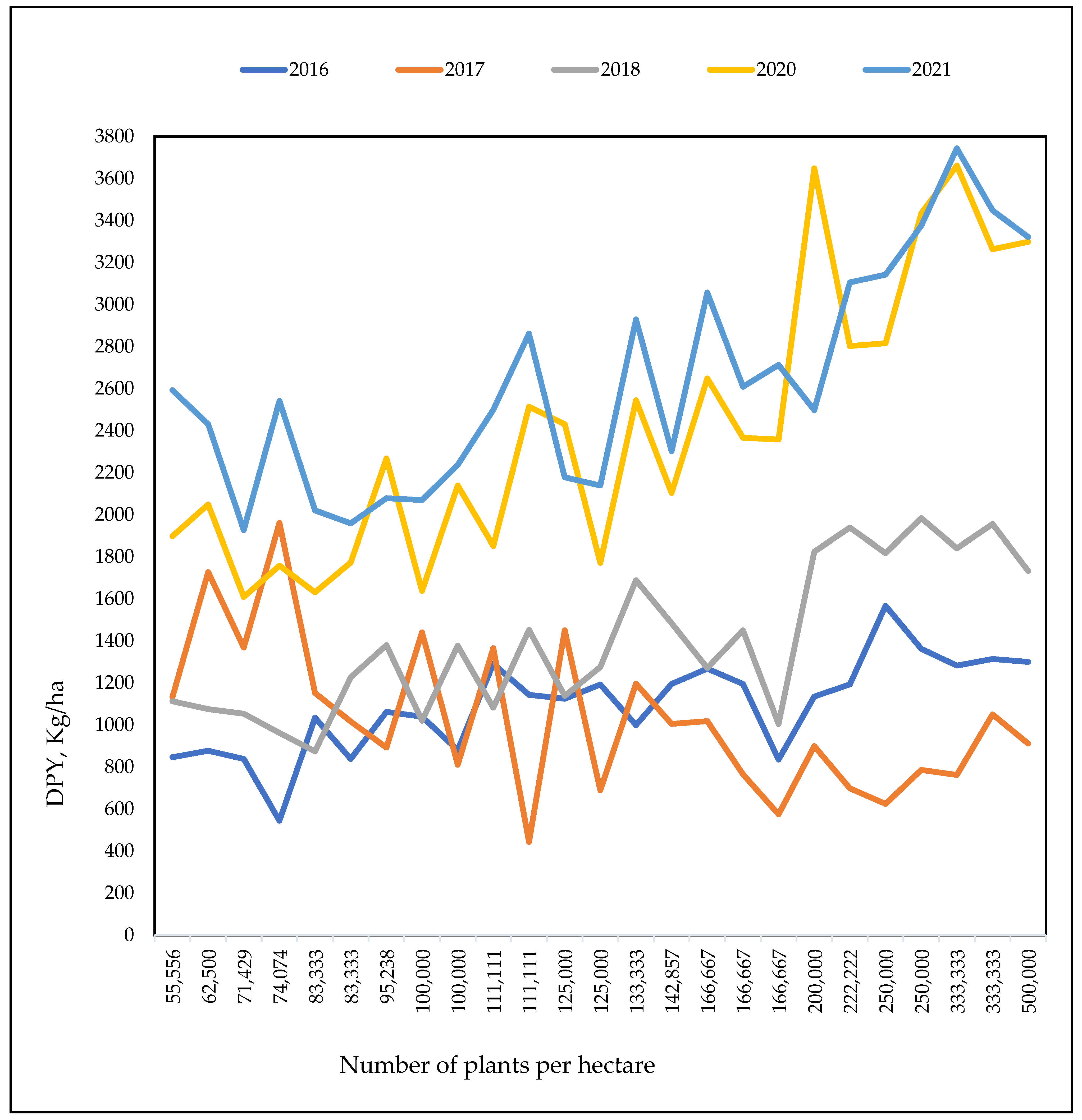
Plant density has a significant impact on groundnut dry pod yield in WCA according to the study, meaning that the current spacing should be revisited. With the exception of 2017, it was obvious that high plant density boosts groundnut dry pod yield throughout both rainy and dry seasons. During the rainy season, dry pod yield was 23.6% higher with 40 cm × 10 cm spacing in 2016, 56% higher with 20 cm × 20 cm spacing in 2018, and 33.2% higher with 40 cm × 10 cm spacing across the two years than the 60 cm × 10 cm spacing which is currently utilized at ICRISAT-WCA. In 2016, there was no significant difference between the control (60 cm × 10 cm) and the best (40 cm × 10 cm) spacings. During the dry season, dry pod yield was 38.2% higher with 30 cm × 10 cm spacing in 2020, 22.4% higher with 30 cm × 10 cm spacing in 2021, and 29.8% higher with 30 cm × 10 cm spacing for the two years than with the standard 60 cm × 10 cm spacing. When the rainy and dry seasons were combined, the 30 cm × 10 cm produced 27.7% more dry pods, followed by 23.1% for 20 cm × 20 cm spacing.

These findings are consistent with those of other researchers, e.g., [11,17,18,19]. Ajeigbe et al. [11] reported that pod yields at 133,333 hills per hectare (75 cm × 10 cm with two plants per hill) were 31% higher than at 66,667 (75 cm × 20 cm with two plants per hill) and 40% higher than at 44,444 hills per hectare (75 cm × 30 cm with two plants per hill) in Nigeria. In Ethiopia, 250,000 plants per hectare (40 cm × 10 cm) and 200,000 plants per hectare (50 cm × 10 cm) were found to be the ideal plant densities for increased seed yield for groundnut cultivars with different architectures [18]. In the Northern Guinea Savannah zone of Ghana, it was observed that the lowest sowing density (80,000 plants per hectare) gave the lowest pod and seed yields in groundnut, compared with medium (120,000 plants per hectare) and high (200,000 plants per hectare) sowing densities, with no significant difference between the latter two densities [20]. They discovered that sowing at a medium density enhanced pod yield by 8–10% compared with sowing at a low density. According to crop simulation studies, increasing the plant density to 400,000 plants per hectare could significantly increase yield in Africa for places where drought is not a limiting issue [17]. Ojelade et al. [19] attributed increased growth and yield of groundnut in narrow intra-row spacing to the reduced weed competition for resources such as light, nutrients, space, and water achieved by the smothering effect of groundnut on late-emerging weeds at narrow compared with wide plant spacing. In our case, the recommended twice weeding was applied, and the increased yield could be attributed to efficient utilization of available resources with an optimum spacing of the plants. However, Dapaah et al. [21] recommended the medium, 166,700 plants per hectare (60 cm × 20 cm with two plants per hill) and 200,000 plants per hectare (50 cm × 20 cm with two plants per hill) plant densities under favorable conditions in the forest–savannah transitional agroecological zone of Ghana.

Outside of Africa, similar observations of narrower spacings for increased groundnut yield have been made. In Bangladesh, for example, a narrower spacing (30 cm × 10 cm) was determined to be optimal for maximum yield for erect (bunch) groundnut varieties, whereas a spreading or semi-spreading groundnut variety required a wider spacing (40 cm × 20 cm) to express its full yield potential [8]. In Turkey, Onat et al. [9] found that increasing plant density enhanced pod yield per hectare. A narrow-row planting (30 cm) gave a significantly higher yield (3739 kg/ha) than wide-row (60 cm) planting (1903 kg/ha) in Pakistan [22]. Plant densities and row spacing of 350,000 plants per hectare (25 cm × 25 cm with two plants per hill) and 400,000 plants per hectare (25 cm × 20 cm with two plants per hill) were found appropriate for high yield in Vietnam [10]. In Australia, Bell et al. [23] reported an increase in total dry matter and pod yields with increasing plant density under fully irrigated conditions, though cultivars differed in their response, with the best cultivar, chico, recording the highest total dry matter and pod yields at 352,000 plants per hectare.

In our study, in 2017, wider spacing (lower plant density) outperformed higher plant density, with 90 cm × 15 cm producing 92.4% more DPY than 60 cm × 10 cm. This finding is in agreement with Wright and Bell [24], and Nandania et al. [25] who reported that increased inter-row space resulted in increased pod yield per hectare. However, the result contradicts with findings by Dapaah et al. [21] who found that in the drier season of 2009, the highest plant density (333,000 plants per hectare) increased pod yield by 29 to 46% and seed yield by 28 to 44% over the lower plant densities, indicating that in drier seasons, higher plant density might be an advantage in moisture conservation once crop canopy closure was achieved.

In the case of DHY, higher yields were obtained for wider spacings during the rainy season, whereas the opposite was true during the dry season. DHY was negatively correlated with DPY during the rainy season while it was positively correlated during the dry season. DHY was 34.5% higher with 90 cm × 15 cm spacing in 2016, 58.4% with 90 cm × 20 cm spacing in 2017, 32% with 90 cm × 15 cm spacing in 2018, and 33.2% with 90 cm × 15 cm spacing across the two years (2016 and 2018) than with the 60 cm × 10 cm spacing. This could be due to 1) a high early leaf spot infection during the rainy season, which resulted in over 70% defoliation at crop maturity stage, and 2) the widely spaced plants having comparatively vigorous growth for increased haulm, which was also evidenced by a large number of pods per plant and seed size. The result for the rainy season contradicts with Ajeigbe et al. [11] who reported that increasing plant density to 133,333 hills per hectare (two plants per hill) increased haulm yield by 14–22% over 44,444 hills per hectare (two plants per hill) and by 7 to 10 % over 66,667 hills per hectare (two plants per hill) in the Sudanian agroecology of Nigeria. However, the results for the dry season were in agreement with Ajeigbe et al. [11]. During the dry season, DHY was 43.9% higher with 30 cm × 10 cm spacing in 2020, 37.9% with 30 cm × 10 cm spacing in 2021, and 40.8% with 30 cm × 10 cm spacing across the two years than the 60 cm × 10 cm spacing. During the dry season, there was no early leaf spot disease incidence or leaf defoliation, and the plants remained green and leafy at harvest.

Further, wider row and plant spacing (i.e., low plant density) demonstrated superior values in the NMP and 100 SW, which could be attributed to compensatory growth due to the availability of better growth resources to the individual plants. However, these values were insufficient to compensate for the low plant density and had a substantial impact on the dry pod yield per hectare. Many other studies have found that increasing the plant spacing (wider spacing) increased the number of pods per plant. In Bangladesh, a higher number of mature pods per plant and a higher dry weight of pods per plant with the widening of row and plant spacing were reported [8]. The reason for this could be that wider spacing allows the plant to use more nutrients and solar energy while reducing competition for all other inputs. In Turkey, reducing plant density resulted in an increased number of pods and weight of pods per plant with the 70 cm × 25 cm and 75 cm × 25 cm planting density yielding the maximum pod weight (97.57 g and 94.83 g) and pod number (96.4 pods and 93.5 pods) per plant for Virginia market types [9]. Similarly, reduced seed yield per plant and number of pods per plant were reported in Sudan with increased plant density attributed to plant competition in high-density plantings [26]. However, because high-density planting produces fewer pods per plant, the pods will be of a similar age and stage of development, making it easy to decide when to harvest [27]. Due to increased uniformity, pods of similar age and stage of development will have a positive impact on post-harvest processes such as shelling, sorting, and subsequent grain quality.

4.2. Effect of Plant Density on Revenue, Net Benefit, and Benefit-to-Cost Ratio

The high DPY and DHY obtained from high plant density in the study were reflected in high revenue and net benefit. For the rainy season, the production value (revenue) was 18.4% higher with 40 cm × 10 cm spacing in 2016, 49.3% with 20 cm × 20 cm spacing in 2018, and 29.9% with 20 cm × 20 cm spacing across the two years compared with the 60 cm × 10 cm spacing. However, the revenue in 2016 from 40 cm × 10 cm was not significantly different from the one obtained with the 60 cm × 10 cm. For the dry season, revenue was 47.9% higher with 30 cm × 10 cm spacing in 2020, 21.6% higher with 30 cm × 10 cm spacing in 2021, and 33.2% higher with 30 cm × 10 cm spacing across the two years than with the 60 cm × 10 cm spacing. Cropping in the dry season generates more revenue than cropping in the rainy season, owing to the higher yield achieved from dry season cropping, which is better managed with the absence of leaf disease burden. When the rainy and dry seasons were combined, the 30 cm × 10 cm yielded a 24.5% increase in revenue. For the rainy season, except for the 20 cm × 10 cm spacing in 2016, the estimates of net benefit showed positive values, indicating financial profitability for all treatments. The net benefit was 30.6% greater with 90 cm × 10 cm spacing in 2016, 86.1% with 50 cm × 15 cm spacing in 2018, and 37.1% with 40 cm × 10 cm spacing across the two years than with the 60 cm × 10 cm spacing. However, the benefit in 2016 from 90 cm × 10 cm was not significantly different from the one obtained with the 60 cm × 10 cm. During the dry season, the net benefit was 51.6% higher with 50 cm × 10 cm spacing in 2020, 21.6% higher with 30 cm × 10 cm spacing in 2021, and 33.3% higher across the two years with 30 cm × 10 cm spacing than with the 60 cm × 10 cm spacing. The net benefit for dry season production was much higher than for rainy season production, implying that investing in dry season production is advantageous provided irrigation facilities are available. The 30 cm × 10 cm provided a 24.4% higher net benefit when the rainy and dry seasons were combined. Considering only seed cost, a spatial arrangement of 30 cm × 10 cm followed by 20 cm × 10 cm yielded the maximum benefit for erect types, while a spatial configuration of 40 cm × 20 cm yielded the maximum benefit, followed by 30 cm × 20 cm for spreading types [8]. In Nigeria, Ajeigbe et al. [11] reported 9 to 27% increased profit for planting at the density of 133,333 hills per hectare (two plants per hill) over 66,667 and 44,444 hills per hectare (two plants per hill). Despite having a high DPY and production value comparable with the 30 cm × 10 cm in our study, the 20 cm × 10 cm (500,000 plants per hectare) had the lowest net benefit due to the high cost of production. This suggests that increasing the density over 333,333 plants per hectare will not increase yield but will instead raise production costs, although Vadez et al. [17] proposed increasing the density to 400,000 plants per hectare.

All of the treatments have a positive benefit-to-cost ratio, or the net benefit from each dollar spent on treatment, with the exception of the 20 cm × 10 cm, which has a negative value in 2016. Wider spacings, in contrast to revenue and net benefit, indicated a higher benefit-to-cost ratio. The benefit-to-cost ratio was 61.6% higher with 90 cm × 10 cm spacing in 2016, 89.3% with 50 cm × 15 cm spacing in 2018, and 43.0% with 90 cm × 10 cm spacing across the two years than with the 60 cm × 10 cm spacing during the rainy season. Similarly, the benefit-to-cost ratio was 41.1% higher with 40 cm × 10 cm spacing in 2020, 11.6% with 90 cm × 20 cm spacing in 2021, and 9.4% with 60 cm × 15 cm spacing across the two years than with the 60 cm × 10 cm spacing. When the rainy and dry seasons were combined, the 60 cm × 15 cm provided a benefit-to-cost ratio of 13.3% higher with the 60 cm × 10 cm spacing. Despite being profitable, all the spacings during the rainy season had a lower ratio (less than unity), with the exception of 90 cm × 10 cm (1.07) and 70 cm × 15 cm (1.0), which were the best options. On the other hand, all the spacings in the dry season production had a higher ratio (more than unity), indicating that each dollar invested in production delivers a net benefit greater than the incurred cost. The 60 cm × 15 cm, 90 cm × 20 cm, and 50 cm × 10 cm spacings with unitary net benefits of 2.62, 2.51, and 2.43, respectively, represent the most cost-effective options. In Bangladesh, the highest benefit-to-cost ratio in terms of solely seed cost was reported for 40 cm × 20 cm spacing [8].

4.3. Implications

This study investigated a wide range of plant densities, from 55,556 plants (90 cm × 20 cm) to 500,000 (20 cm × 10 cm) plants per hectare (almost a 10-fold range), in comparison to earlier studies. Across years and seasons, the plant density of 333,333 plants per hectare (30 cm × 10 cm) proved to be the best for increased dry pod yield, production value, and net benefit. The DPY, 2633 kg/ha (1562 kg/ha and 3703 kg/ha during rainy and dry seasons) for 30 cm × 10 cm, did not differ significantly from the 2539 kg/ha obtained from 20 cm × 20 cm (250,000 plants per hectare), and the 2496 kg/ha from 20 cm × 15 cm (333,333 plants per hectare), and the latter two not being significantly different from 2414 kg/ha from 20 cm × 10 cm (500,000 plants per hectare). The USD 1510 per hectare production value (USD 847.4 and USD 2173 during rainy and dry seasons, respectively) and USD 888.4 per hectare (USD 266.5 and USD 1510.2 during rainy and dry seasons, respectively) from the 30 cm × 10 cm spacing were significantly different from values obtained from other plant densities. Considering each season separately, the 40 cm × 10 cm (250,000 plants per hectare) proved to be the optimum spacing with 1693 kg/ha DPY, USD 890.9 production value, USD 403.5 net benefit and 0.83 benefit-to-cost ratio during the rainy season. The 30 cm × 10 cm (333,333 plants per hectare) was the best with 3703 kg/ha DPY, USD 2173 revenue, and USD 1510.2 net benefit at a 2.28 benefit-to-cost ratio during the dry season under an irrigated condition. In general, a higher benefit-to-cost ratio was observed with lower plant densities. However, increased yield, production value, and net benefit are more important to smallholder farmers than the benefit-to-cost ratio. Because a portion of the crop is consumed at home, a high yield per hectare means more groundnut is accessible for home consumption, thereby enhancing household nutrition and food security.

Increasing plant density would necessitate more seeds and likely more labor, hence increased production cost on the part of growers [17] but possibly less cost of weeding as the close canopy reduces light penetration, thereby suppressing weed growth for reduced weed biomass [16]. In our study, seed cost accounted for 12% and 9.3% (90 cm × 20 cm) to 39.6% and 35.6% (20 cm × 10 cm) of the overall production cost during the rainy and dry seasons, respectively. The seed cost for the 30 cm × 10 cm accounted for 35.6% and 31.3% during the rainy and dry seasons, respectively, compared with 26.2% and 21.7% for the 60 cm × 10 cm, which is close to a 10% increase in the total cost. The labor cost accounted for 28.7% and 22.9% (90 cm × 10 cm) to 49.3% and 43.5% (20 cm × 20 cm), during the rainy and dry seasons, respectively. The labor cost for 30 cm × 10 cm accounted for 36.5% and 32% during the rainy and dry seasons, respectively, compared with 33.5% and 27.75% for 60 cm × 10 cm, resulting in about 3–4% increase in the total cost. The seed and labor cost increase caused by increased plant density is more than offset by the increased production value and net benefit. However, mechanization in row-making, planting, weeding, and harvesting could lower production costs, resulting in a bigger net benefit. According to Ajeigbe et al. [11], farmers in West Africa plant grain crops in rows 75 cm apart because most tractor and animal-drawn ridgers are fixed at a width of 75 cm, leaving farmers with no option to reduce row spacing. Even though research institutes and large commercial farms may be able to source adjustable ridgers, smallholder farmers may find it difficult to get suitable ridgers, planters, and harvesters for narrow row spacings such as 20 cm or 30 cm. In such circumstances, sowing two seeds per hill, as done in Nigeria, while preserving the 60 cm × 10 cm spacing may be used, albeit this is not ideal because two plants per hill may promote competition for space, lowering yield. Alternatively, to limit competition between plants in a hill, the 60 cm spacing between rows might be retained but the space between plants is reduced to 5 cm (dry season) or 7.5 cm (rainy season) instead of 10 cm. However, adjusting the spacing to increase plant density should be easy for the majority of smallholder farmers who use animal-drawn cultivators and manual drillers, as well as those who use hoes and hand drilling.

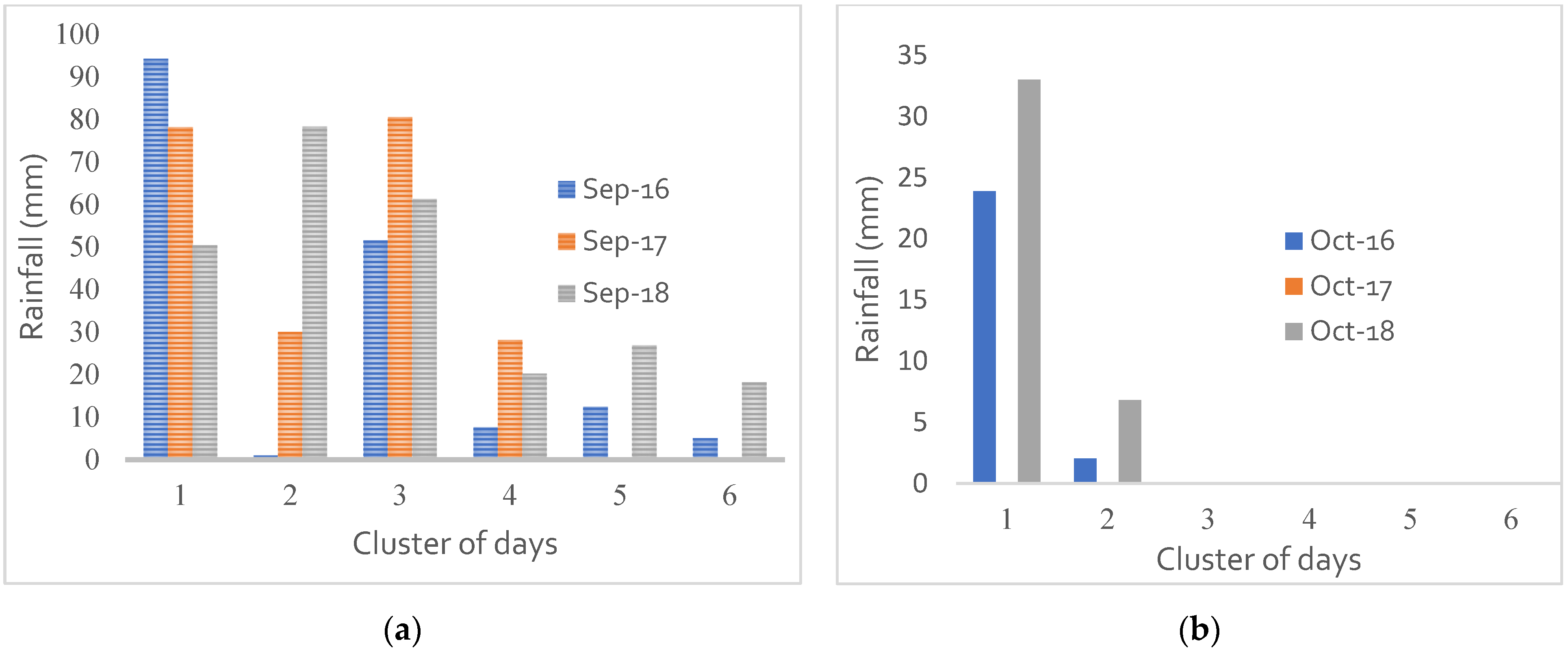
The study also revealed that high plant density may not be suitable for moisture stress scenarios such as those experienced in 2017 when groundnut was hit by a terminal drought. Although the Sudan Savannah agroecology receives relatively adequate rainfall for groundnut cultivation in terms of quantity, terminal drought remains a challenge [28]. Rainfall distribution can be irregular, and with the current climate change and variability in the region, this is projected to get worse. Further, while early groundnut planting at the onset of rain is recommended, many farmers, particularly women, lack the necessary planting equipment such as a plow to plant groundnut on time. Sorghum and pearl millet, which are the key staples, are given the priority in planting. As a result, groundnut planting is frequently delayed, exposing groundnut to terminal drought. In the Sahelian agroecology, such as the Kayes and Segou regions of Mali, terminal drought poses a serious problem to groundnut production. The findings, although from only one year, suggest that plant densities of 74,000 plants per hectare (90 cm × 15 cm) to 111,111 plants per hectare (60 cm × 15 cm; 90 cm × 10 cm) may be adequate for locations where terminal drought occurs. Simulation models suggested that, for latitudes above 12–13° N, increasing population density may not enhance yield due to drought [17]. More research at representative sites for at least two rainy seasons will be useful in validating the optimal plant density for the Sahel agroecology. Furthermore, in both the Sahel and Sudan Savannah agroecologies, reliable weather forecasting and its availability to farmers will be critical in making planting density decisions for a specific year during the rainy season.

5. Conclusions

Based on the findings of this study and linking pieces of evidence from other countries in the region, we recommend increasing plant density to at least 222,000 plants per hectare (i.e., 30 cm × 15 cm spacing) for rainfed crops with appropriate planting time and 333,000 plants per hectare (30 cm × 10 cm spacing) for irrigated (dry season) crops for groundnut production in the Sudan Savannah agroecology of WCA.

References

1. FAOSTAT. FAOSATAT, Statistical Data Base; Visited on 29/05/2021; Food and Agricultural Organizations of the United Nations: Rome, Italy, 2021. [Google Scholar]
2. Sinare, B.; Miningou, A.; Nebié, B.; Eleblu, J.; Kwadwo, O.; Traoré, A.; Zagre, B.; Desmae, H. Participatory analysis of groundnut (Arachis hypogaea L.) cropping system and production constraints in Burkina Faso. J. Ethnob. Ethnom. 2021, 17, 2. [Google Scholar] [CrossRef] [PubMed]
3. Anim-Somuah, H.; Henson, S.; Humphrey, J.; Robinson, E. Strengthening Agri-Food Value Chains for Nutrition: Mapping Value Chains for Nutrient-Dense Foods in Ghana; IDS Evidence Report No. 2, Reducing Hunger and Undernutrition; Institute of Development Studies (IDS): Brighton, UK, 2013. [Google Scholar]
4. Wagh, V.D.; Deore, B.R. Ready to Use Therapeutic Food (RUTF): An Overview. Adv. Life Sci. Health 2015, 2, 1–14. [Google Scholar]
5. GAIN. Revitalization of the Groundnut Sector in West Africa (Gambia, Guinea Bissau and Senegal). Global Agricultural Information Network (GAIN). Available online: http://gain.fas.usda.gov/Recent%20GAIN%20Publications/Revitalization%20of%20the%20Groundnut%20sector%20in%20West%20Africa_Dakar_Senegal_12-3-2010.pdf (accessed on 18 November 2016).
6. Ndjeunga, J.; Ibro, A.; Cisse, Y.; Ben, A.; Miko, I.; Moutari, A.; Abdoulaye, A.; Kodio, O.; Mohammed, S.G.; Echekwu, C.A. Characterizing Village Economies in Major Groundnut Producing Countries in West Africa: Cases of Mali, Niger and Nigeria; ICRISAT: Patancheru, India, 2010; p. 89. [Google Scholar]
7. Janila, P.; Mula, M.G. Cultural Management Practices of Groundnut; ICRISAT Center: Patancheru, India, 2015. [Google Scholar]
8. Howlader, S.H.; Bashar, H.M.K.; Islam, M.S.; Mamun, M.H.; Jahan, S.M.H. Effect of Plant Spacings on the Yield and Yield Attributes of Groundnut. Int. J. Sustain. Crop Prod. 2009, 4, 41–44. [Google Scholar]
9. Onat, B.; Bakal, H.; Gulluoglu, L.; Arioglu, H. The Effects of Row Spacing and Plant Density on Yield and Yield Components of Peanut Grown as a Double Crop in Mediterranean Environment in Turkey. Turk. J. Field Crops 2017, 22, 71–80. [Google Scholar] [CrossRef]
10. Minh, T.X.; Thanh, N.C.; Thin, T.H.; Thi, T.N.; Giang, N.T.H. Effects of Plant Density and Row Spacing on Yield and Yield Components of Peanut (Arachis hypogaea L.) on the Coastal Sandy Land Area in Nghe An Province, Vietnam. Indian J. Agr. Res. 2021, 55, 468–472. [Google Scholar] [CrossRef]
11. Ajeigbe, H.A.; Kamara, A.Y.; Kunihya, A.; Inuwa, A.H.; Adinoyi, A. Response of Groundnut to Plant Density and Phosphorous Application in the Sudan Savanna Zone of Nigeria. Int. J. Biosci. 2016, 9, 291–302. [Google Scholar]
12. Ajeigbe, H.A.; Vabi, M.B.; Inuwa, A.H.; AbdulAzeez, T.; Akinseye, F.M. Handbook on Improved Agronomic Practices of Groundnut Production in North-East Nigeria; ICRISAT: Kano, Nigeria, 2020; p. 17. [Google Scholar]
13. Zakaria, J. Personal Communication; Institute of Agricultural Research: Kaduna, Nigeria, 2021. [Google Scholar]
14. DNA. Manuel de Procedure Pour L’inscription des Varietes au Catalogue National des Especes et Varietes; Direction Nationale de l’Agriculture (DNA), Ministere de l’Agriculture: Bamako, Mali, 2010.
15. Oteng-Frimpong, R.; Rasheed, M.A.; Rashid, I.A.; Denwar, N.N.; Nutsugah, S.K. Growing Groundnut Profitably in the Guinea Savanna of Ghana. In Leaflet; P.O. Box TL52; CSIR-Savanna Agricultural Research Institute: Tamale, Ghana, 2017. [Google Scholar]
16. Rahman, N.A.; Bekele, K.; Fred, K.; Irmgard, H.-Z. Optimal spacing for groundnuts in smallholder farming systems. In Africa RISING Technology Brief; IITA: Ibadan, Nigeria, 2021. [Google Scholar]
17. Vadez, V.; Halilou, O.; Hissene, H.M.; Sibiry-Traore, P.; Sinclair, T.R.; Soltani, A. Mapping Water Stress Incidence and Intensity, Optimal Plant Populations, and Cultivar Duration for African Groundnut Productivity Enhancement. Front. Plant Sci. 2017, 8, 432. [Google Scholar] [CrossRef] [PubMed] [Green Version]
18. Gabisa, M.; Tana, T.; Elias, U. Effect of planting density on yield components and yield of Groundnut (Arachis hypogaea L.) varieties at Abeya, Borena Zone, Southern Ethiopia. IJSEAS 2017, 3, 1–18. [Google Scholar]
19. Ojelade, O.B.; Lagoke, S.T.; Adigun, J.A.; Babalola, O.A.; Daramola, O.S.; Osipitan, O.A. Intra-Row Spacing and Weed Control Influence Growth and Yield of Groundnut (Arachis hypogea L.). Adv. Agr. Sci. 2018, 6, 1–11. [Google Scholar]
20. Naab, J.B.; Tsigbey, F.K.; Prasad, P.V.V.; Boote, K.J.; Bailey, J.E.; Brandenburg, R.L. Effects of sowing date and fungicide application on yield of early and late maturing peanut cultivars grown under rainfed conditions in Ghana. Crop Prot. 2005, 24, 325–332. [Google Scholar] [CrossRef]
21. Dapaah, H.K.; Mohammed, I.; Awuah, R.T. Phenological development and yield of three groundnut varieties as influenced by plant density in a Forest-savanna Transition Zone. Int. J. Agr. Res. 2014, 9, 87–98. [Google Scholar] [CrossRef] [Green Version]
22. Ahmad, N.; Rahim, M.; Khan, U. Evaluation of Different Varieties, Seed Rates and Row Spacing of Groundnut, Planted under Agro-Ecological Conditions of Malakand Division. J. Agron. 2007, 6, 385–387. [Google Scholar] [CrossRef] [Green Version]
23. Bell, M.J.; Harch, B.; Wright, G.C. Plant population studies on peanut (Arachis hypogaea L.) in subtropical Australia. I. Growth under fully irrigated conditions. Aust. J. Exp. Agric. 1991, 31, 535–543. [Google Scholar] [CrossRef]
24. Wright, G.C.; Bell, M.J. Plant population studies on peanut (Arachis hypogaea L.) in subtropical Australia. 3. Growth and water use during a terminal drought stress. Aust. J. Exp. Agric. 1992, 32, 197–203. [Google Scholar] [CrossRef]
25. Nandania, V.A.; Mohdawadia, M.M.; Patel, J.C.; Sadaria, S.G.; Patel, B.S. Response of rainy season bunch groundnut (Arachis hypogaea L.) to row spacing and seed rate. Indian J. Agron. 1992, 37, 597–599. [Google Scholar]
26. El Naim, A.M.; Eldouma, M.A.; Ibrahim, E.A.; Zaied, M.M.B. Influence of Plant Spacing and Weeds on Growth and Yield of Peanut (Arachis hypogaea L) in Rain-fed of Sudan. Adv. Life Sci. 2011, 1, 45–48. [Google Scholar] [CrossRef] [Green Version]
27. Okello, D.K.; Kaaya, A.N.; Bisikwa, J.; Were, M.; Oloka, H.K. Management of Aflatoxins in Groundnuts: A manual for Farmers, Processors, Traders and Consumers in Uganda; National Agricultural Research Organisation: Entebbe, Uganda, 2010; ISBN 978-9970-401-00-0. [Google Scholar]
28. Sanogo, O. Early Generation Selection for Drought Related Traits in Groundnut (Arachis hypogaea L.) in Mali. Ph.D. Thesis, University of Ghana, Accra, Ghana, 2016. [Google Scholar]
Figure 1. Total rainfall (a) September and (b) October with 5 days cluster in 2016, 2017, and 2018.
Agronomy 12 01474 g001
Figure 2. Trend of dry pod yield (kg/ha) with increasing plant density per hectare of spacing treatments for each year. The dry pod yield increased with increasing plant density for 2016, 2018, 2020, and 2021. In 2017, the dry pod yield decreased when plant density was increased.
Agronomy 12 01474 g002