Article

Sustainable Production of Barley in a Water-Scarce Mediterranean Agroecosystem

by
José Antonio Martínez-López
1,
Ramón López-Urrea
2,
Ángel Martínez-Romero
1,
José Jesús Pardo
1,
Jesús Montero
1 and
Alfonso Domínguez
1,*
1
Centro Regional de Estudios del Agua (CREA), Universidad de Castilla—La Mancha (UCLM), 02071 Albacete, Spain
2
Instituto Técnico Agronómico Provincial (ITAP), Parque Empresarial Campollano, 2ª Avenida–Nº 61, 02007 Albacete, Spain
*
Author to whom correspondence should be addressed.
Agronomy 2022, 12(6), 1358; https://doi.org/10.3390/agronomy12061358
Submission received: 11 May 2022 / Revised: 30 May 2022 / Accepted: 1 June 2022 / Published: 3 June 2022
(This article belongs to the Special Issue Selected Papers from 11th Iberian Agroengineering Congress)

Abstract

:
Scarcity of water resources is one of the main constraints on agricultural activity in arid and semi-arid areas. Despite the great technological development over recent decades, farmers are demanding methodologies and tools adapted to their training, management restrictions, and economic capacity. To tackle these challenges, the sustainable production in water-limited environments of Mediterranean agroecosystems (SUPROMED) project combines, in an online platform, a set of models and methodologies for more efficient management of water, energy, and fertilizers. A two-year trial (2020–2021) was conducted in the Castilla-La Mancha region (Spain) to demonstrate, for a barley crop, the effectiveness of SUPROMED as a farm management support tool. The impact of transferring the model for the economic optimization of irrigation water use at farm level (MOPECO model) irrigation scheduling among other methods and tools, integrated in the SUPROMED platform, to farmers was determined by analyzing a set of productive, economic, and environmental key performance indicators (KPIs). The KPIs were selected to show farmers how the efficient use of productive factors could improve the profitability of their farms, thus reducing the impact of agriculture on the environment. In 2020, the management plan proposed by SUPROMED achieved the same yield as traditional management using 32% less water and resulting in a 13% and 66% improvement in gross margin and gross economic irrigation water productivity, respectively. In 2021, the management implemented by a farmer trained in the use of the tools and methodologies in the SUPROMED platform showed improvements in most of the KPIs analyzed, achieving similar results to those obtained by SUPROMED during 2020. The results are promising, indicating that the tools and models proposed in SUPROMED can be easily used by farmers and can improve the economic and environmental sustainability of Mediterranean agroecosystems. The involvement of public administrations, together with local researchers and technicians, is required for the effective promotion and use of these methodologies by the productive sector.

1. Introduction

The Mediterranean area is one of the world’s richest regions in ecosystems. However, it is also one of the most vulnerable zones due to irregular rainfall distribution throughout the year and water scarcity caused by frequent drought periods [1]. Thus, the lack of water resources is one of the main handicaps for agriculture in this area [2]. In addition, the farming sector is greatly conditioned by numerous economic (e.g., harvest price and labor cost), political (e.g., laws for the protection of the environment), social (e.g., food security and maintenance of rural population), technical (e.g., machinery and crops), and environmental (e.g., climate, soil, and diseases) factors. Moreover, despite the great technological development over recent decades (e.g., artificial intelligence techniques, remote sensing, soil moisture sensors, online irrigation tools, thermal images, photosynthesis analyzer, stomatal conductance measurements, etc.), farmers are demanding methodologies and tools adapted to their training, management restrictions, and economic capacity for a real improvement in the use of the inputs at the farm level.
The lack of tools and/or irrigation advisory services for determining the irrigation requirements of crops at the farm level, the lack of knowledge about the irrigation system [3,4,5], the low price of harvests in the international market, and climate change have all led to an excessive use of resources, such as groundwater and energy, to compensate for these shortages, decreasing the profitability of farms located in Mediterranean areas [6,7].
Tackling the challenges of this situation requires a combination of methodologies and technologies that include enhancing the efficiency of the use of natural resources, improving the design and management of the means of production, developing and transferring technology and knowledge to producers, analyzing scenarios to advise farmers and technicians about the most suitable strategies for dealing with extreme situations, and providing decision makers with tools and reports to help develop policies to improve the resilience of agricultural systems to these threats [8].
Currently, artificial intelligence (AI) techniques with high data processing and machine learning capabilities [9,10,11] can be applied in irrigation hydraulic management [12], hyperspectral image processing [13] to estimate or predict climate data, optimal resource distributions (water or fertilization) [14], or environmental impact management [15]. In the same way, many crop simulation models and tools have been developed in order to act as decision support systems for field crops to be used by managers, technicians, and/or farmers [16,17,18,19]. These models often require a large number of input variables and parameter values that are not easily available to end users. In this sense, the model for the economic optimization of irrigation water use at farm level (MOPECO model) [20] was designed to maximize the profitability of irrigated farms in water-scarce arid and semi-arid areas through efficient use of irrigation water [21] and the available cultivable area [5]. This model can be used in many irrigable areas by calibrating a small number of crop parameters. To generate irrigation schedules, MOPECO takes into account factors such as the total available irrigation water, the effect of irrigation uniformity [5], the electrical conductivity of irrigation water [22], and the water deficit sensitivity at the different crop growth stages, among others [21]. MOPECO has already been calibrated for the most common crops in the Castilla-La Mancha region (Spain) [22,23,24,25,26,27] and other areas of the world [27,28,29,30].
Sustainable production in water-limited environments of Mediterranean agroecosystems (SUPROMED) is a three-year project (2019–2022) funded by Partnership for Research and Innovation in the Mediterranean Area (PRIMA), in which ten partners from five different countries (Spain, France, Greece, Lebanon, and Tunisia) have participated. The project is intended to enhance the economic and environmental sustainability of Mediterranean farming systems through a more efficient management of water (evaluation of the irrigation systems and proper irrigation scheduling taking into account weather forecast and soil moisture), land (good agricultural practices and optimal distribution of crops), energy (audits and solar power), and fertilizers (soil analysis and nutrient balance). For this purpose, SUPROMED combines various models and tools, such as MOPECO [20] or design of pressurized irrigation (DOPIR) [31], in order to properly manage inputs (mainly water, energy, and fertilizers). These tools were simplified and adapted for farmers and technicians and implemented in an end-user online platform intended to provide effective advice for more sustainable and profitable crop management. Moreover, the project proposes several complementary methodologies, such as evaluation of the irrigation systems, control of the actual amount of water supplied at each irrigation event, monitoring of the soil moisture content, and fertilization based on the nutrient balance, among others. All the models were developed by the partners participating in the project, as is the case for the fertilization requirement calculator tool, MOPECO, DOPIR, and PRESUD models (University of Castilla-La Mancha, Spain), the irrigation scheduling tool IREY (Institut National des Grandes Cultures, Tunisia), weather forecast (3DSA, Greece), and the agroclimatic zone and evapotranspiration calculation using remote sensing tools (University of Thessaly, Greece). The proposed methodologies are those widely accepted across the world, such as the evaluation of irrigation systems [32,33,34], the determination of ETo by using the data registered by an agroclimatic station [35], the protocol for carrying out an energy audit [36], the determination of the real amount of water provided by an irrigation system using a pressure transducer, or the monitoring of soil water content using soil moisture sensors [37,38,39]. The methodology was tested in three demo-sites located in eastern Mancha (Spain), Sidi Bouzid (Tunisia), and Bekaa Valley (Lebanon). The main partners in these areas are Instituto Técnico Agronómico Provincial (ITAP), Institut National de Recherche en Génie Rural Eaux et Fôrets (INRGREF), and University of Lebanon, Faculty of Agronomy (ULFA), respectively. Three more enterprises participated in the project to develop the online platform (Grupo HISPATEC, Spain), carrying out the socio-economic analysis on the impact of the project at local, regional, and Mediterranean basin levels (Difaf, Lebanon), and disseminating the results (SEMIDE, France). A more detailed description of the project and the access to the online platform are available on the SUPROMED webpage (www.supromed.eu accessed on 30/34/2022).
Barley is the 13th most produced crop in the world and 4th in harvested area, with 1570 million Mg and 51.6 million ha, respectively [40]. Europe accounts for 60% of world production with 46% of the global area [40]. Barley is the most widely cultivated crop in Spain, with around 11 million Mg produced in 2.75 million ha, of which 0.36 million are irrigated [41]. CLM is the second largest producing region, with 26% of the national total (2.89 million Mg), cultivating around 0.79 million ha, of which 13% is irrigated, mainly using sprinkler irrigation systems [41]. Despite its low profitability, barley is a key crop in the management of crop rotation, preceding other more profitable crops, such as garlic. Moreover, the low availability of water in many areas is causing farmers to demand tools and models to perform adequate irrigation scheduling, avoiding excesses of irrigation water that may compromise crop profitability.
The main objective of this work was to demonstrate the impact of applying the models and methodologies adapted to farmers in SUPROMED on the sustainability and profitability of a barley crop in comparison with the traditional management of this crop in Castilla-La Mancha. The following secondary objectives were proposed: (1) to determine a set of productive, economic, and environmental key performance indicators (KPIs). The KPIs were selected to show farmers how the efficient use of productive factors can improve the profitability of their farms and reduce the impact of agriculture on the environment; (2) in Year 1, to monitor four farms dedicated to the cultivation of barley and manage a subplot within one of the monitored farms by using the SUPROMED methodologies. In Year 2, (3) to monitor the management of one farm after training the farmer in the use of the methodologies in SUPROMED; and (4) to compare the monitoring results of the two years using the KPIs for assessing the impact of using the tools in SUPROMED and their ability to be used by farmers under real management conditions.

2. Materials and Methods
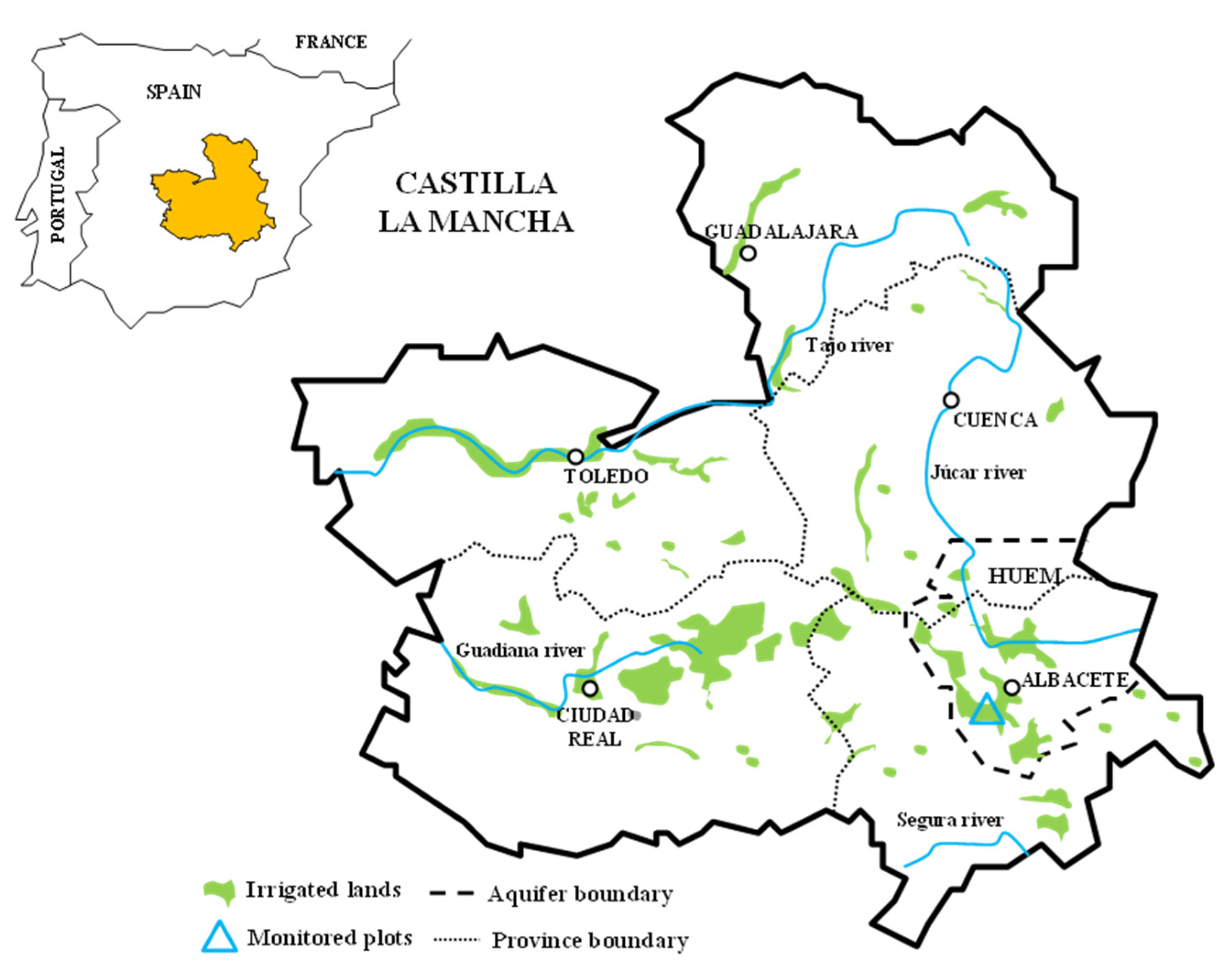
2.1. Study Area

The study was carried out during the 2020 and 2021 growing seasons, in various barley plots located in the hydrogeological unit of eastern Mancha (HUEM) (CLM, Spain) (Figure 1). This agroecological system is characterized by a Mediterranean climate [42] (MeTE), occupies an area of 8500 km2, and supplies irrigation water to more than 110,000 ha. Around 95% of the irrigable area is equipped with pressurized irrigation systems (mainly solid set, center pivot systems, and surface drip irrigation systems), with around 4000 m3 ha−1 being the average yearly water allocation for annual crops in the area.
In the study area, the average daily maximum temperature occurs in summer (33 °C), with great seasonal variability in mean daily temperature (3.8 °C in January and 24.4 °C in July). Long-term mean annual precipitation is 360 mm (mostly concentrated in the autumn and spring months) and mean cumulative annual reference evapotranspiration (ETo) is around 1300 mm.
The typical soils in the area are classified as “Torriorthent” [43]. A petrocalcic horizon is found at a depth of 0.5 to 0.7 m, while the first horizons have a clay loam texture with low to medium levels of soil organic matter.

2.2. Description of Monitored Barley Plots

In 2020, five plots of barley (Hordeum vulgare L., cv. Planet) belonging to four different farmers were monitored. One of the farmers was selected as a “Leader” farmer (LEA), being one of the best-trained and highest-producing farmers in the area. Consequently, in order to compare traditional management and that proposed by SUPROMED (SUP), two plots on his farm, with similar characteristics, were monitored: one managed by LEA and the other by SUP. The other three selected farmers, who we called “Average”, were producers with a training level and a way of managing their farms that is representative of the area (AVE 1, AVE 2, and AVE 3) (Table 1). In 2021, only one barley plot managed by the Leader farmer using SUPROMED tools (LEASUP) was monitored to quantify the improvement capacity of individual farmers when using the proposed methodologies. The relatively low number of monitored barley plots was conditioned by the total number of crops and plots monitored in the eastern Mancha agricultural system. Thus, during the three years of the project, 8 different crops (vegetables, field crops, and fruit trees and vines) cultivated in 39 plots located in 16 farms were monitored. The aim was to validate the proposed methodologies and assess the impact of SUPROMED for a wide range of crops, management conditions, and types of farmers. A similar methodology was used in the other two demo-site areas.
In each monitored barley plot, the area delimited by a set of four sprinklers representing the average conditions of the sector was selected to monitor the experiment.
Before sowing, the soil profile of each demonstrative commercial plot was sampled to determine the effective soil depth and physical (texture) and chemical (nutrient content) properties. Soil analyses were used by MOPECO to determine the irrigation scheduling and fertilization by SUP management and to simulate the farmers’ irrigation schedules.
The average soil depth was 50 cm, with the exception of AVE 2, where it was 70 cm, limited by a petrocalcic horizon. The texture was classified as clay loam, while pH was basic (between 8.4–8.6). SUP and LEA plots had the lowest organic matter content (1.62% vs. 2.47% in the other plots) and higher contents of carbonates (40.82%) and active limestone (10.72%).

2.3. Irrigation System

The irrigation system of all monitored plots is a fixed solid set sprinkler irrigation system. During the initial stage of crop growth, an evaluation of the four irrigation systems was carried out to characterize the spatial distribution of the water applied by the irrigation system and to determine the actual amount of water applied at each irrigation event at working pressure. All this information (Table 2) was used by the SUP team to calculate the proper irrigation scheduling and to improve the uniformity of the SUP plot, if necessary.
The evaluations were performed using the methodology proposed by [32], considering the established standards [33].
To compute the soil water balance using the MOPECO model, a general irrigation application efficiency of 80% was assumed in all cases. This value was based on values for Christiansen’s coefficient of uniformity (CU) obtained in the evaluations of the irrigations systems (most of them between 85–87%, Table 2), and on the low evaporation and drift losses considered due to irrigation events typically occurring during the night.

2.4. Irrigation Scheduling

The “MOPECO irrigation scheduling” tool (https://crea.uclm.es/siar/siarpr/ (accessed on 7 February 2022)) is a simplification for farmers and technicians of the MOPECO model for researchers, which determines the irrigation scheduling of a crop by using the simplified daily soil water balance proposed by FAO-56 [35,44]. The irrigation scheduling module requires soil data (texture, depth, and stone content), climatic data (temperature, ETo, and rainfall), crop parameters (crop coefficient (Kc), duration of crop growth stages in cumulative growing degree days (GDD), lower (TL) and upper (TU) developmental threshold temperatures, and evapotranspiration group) (Table 3), and irrigation system data (efficiency and precipitation rate).
To generate irrigation schedules, MOPECO updates the daily water balance considering the actual amount of water received by the crop (irrigation or rainfall) and the actual weather data. In addition, MOPECO uses the seven-day forecast climatic data provided by the National Institute of Meteorology (INM) [47] and the actual phenological stage of the crop to calculate the irrigation water requirements of the crop for the next week.
The meteorological variables used for the proper determination of the irrigation requirements of the crop were measured by an automated weather station IMETOS 3.3 (Pessl Instruments, Weiz, Austria), positioned on the LEA farm, at no more than 1 km distance from the rest of monitored plots. Reference evapotranspiration (ETo) was calculated by using the Penman–Monteith FAO 56 equation [35] since previous lysimeter studies in the same area reported good performance of this method [48,49], while the effective precipitation was estimated using the United States Department of Agriculture (USDA) methodology “curve number 2” [50,51].

2.5. Plot Monitoring

Over the two experimental seasons, crop phenology was monitored weekly by following the BBCH scale [45] to fit the irrigation scheduling and supply fertilizers at the proper time.
Initial soil water moisture was determined at the beginning of the crop cycle using the gravimetric technique. In each monitored plot, we installed a pressure transducer (Pessl Instruments Pipe Pressure, Weiz, Austria), previously calibrated over a range of 0–10 bar, and a soil moisture probe with 6 sensors with 10 cm spacing (Drill&Drop, Sentek, Australia), both connected to a data logger (ECO D3, Pessl Instruments, Weiz, Austria). The pressure transducer was installed in the rise pipe of the representative sprinkler to monitor the duration and the water applied in each irrigation event. The soil moisture probe was placed in a representative area according to the results of the irrigation system evaluations to monitor the evolution of the volumetric soil water content. The average daily volumetric content measured by the probes was transformed to available water and compared with the available soil water simulated by the MOPECO tool.

2.6. Key Performance Indicators (KPIs)

For comparing the traditional management of the farms with the proposed by using the methodologies and tools in SUPROMED, different key performance indicators (KPIs) were calculated. All the KPIs were based on the final yield obtained in the monitored plots. Thus, once the crop reached physiological maturity, six 0.5 m × 0.5 m random samples were collected in the control area of each monitored subplot to determine the yield. Grain yields were normalized to standard commercial yield (12% moisture content). In 2020, Duncan’s test [52] was performed to determine whether significant differences (p < 0.05) existed between different management types. The KPIs allowed us to assess how efficient the farmers and SUPROMED were, in economic and environmental terms, in their use of the inputs. The selection of these KPIs was based on the hypothesis that the best way to reduce the impact of agriculture on the environment is by demonstrating to farmers that the efficient use of productive factors can improve the profitability of their farms [53,54,55,56].
  • Gross margin (GM) (EUR ha−1), using the information provided by farmers:
GM = Y a PV Cv I g Cw + Subs  
where: GM: gross margin (EUR ha−1); Ya: yield (kg ha−1); Pv: sale price (EUR kg −1), (0.15 EUR kg−1 during 2020 [57], and 0.21 in 2021 [58]); Cv: variable costs (EUR ha−1) (all these cost data were provided by the farmers); Ig: gross irrigation water applied (m3 ha−1); Cw: water cost (EUR m−3) (0.12 EUR m−3 [31]); Sub: subsidies (EUR ha−1) (280 EUR ha−1) (provided by the farmers)
  • Irrigation water productivity (WPI) (kg m−3):
WP I = Y a I g
where WPI: irrigation water productivity (kg m−3); Ya: grain yield (12% moisture) (kg ha−1); Ig: gross irrigation (m3 ha−1).
  • Crop water productivity (WPc) (kg m−3):
WP c = Y a ET a
where WPc: crop water productivity (kg m−3) Ya: commercial grain yield (12% moisture) (kg ha−1); ETa: actual evapotranspiration (m3 ha−1).
  • Net economic irrigation water productivity (NEWP) (EUR m−3):
NEWP = GM ( I N + Re )
where: NEWPI: net economic water productivity (EUR m−3); GM: gross margin (EUR ha−1); IN: net irrigation (m3 ha−1); Re: effective rainfall (m3 ha−1)
  • Gross economic irrigation water productivity (GEWPI) (EUR m−3):
GEWP I = GM I g
where: GEWPI: gross economic irrigation water productivity (EUR m−3); GM: gross margin (EUR ha−1); Ig; gross irrigation (m3 ha−1).
  • Agronomic productivity of nitrogen (APN) (kg NU−1) calculated as:
APN = Y a NU
where: APN: agronomic productivity of nitrogen (kg NU−1); Ya: grain yield (12% moisture) (kg ha−1); NU: nitrogen units applied (NU ha−1).
  • Water footprint (WF)
The water footprint of the barley cropping process (WFtotal) was analyzed as the sum of the green (WFgreen), blue (WFblue), and grey (WFgrey) components:
WF total = WF Green + WF Blue + W Grey  
WF green = ETa green Y a
WF Blue = ETa blue Y a
WF Grey = α AR C maximum C Natural Y a
where WF: water footprint (m3 kg−1); ETa: actual evapotranspiration (m3 ha−1), where ETagreen: water in natural processes evapotranspirated (m3 ha−1) and ETablue: irrigation water evapotranspirated (m3 ha−1); Ya: grain yield (12% moisture) (kg ha−1); the grey component refers to irrigation water to reduce the concentration of pollutants (m3 ha−1). The legislation in the area considers nitrates as the elements that define the fresh and groundwater pollution [55]; α: fraction of applied chemical substances reaching freshwater bodies (dimensionless), in this case, 0.08 [56]; AR: chemical substances applied on or in the soil (kg ha−1), in this case, the amount of N applied to the plots was used; Cmaximum: maximum acceptable concentration (kg m−3), in this case, 50 mg L−1, Cnatural: natural concentration in the receiving water body (that would occur if there were no human disturbances), in this case, 37.3 mg L−1 [59].

3. Results and Discussion

3.1. Evaluation of the Irrigation System

The evaluation of the irrigation system (Table 2) showed that all monitored plots, except AVE 3, had good distribution uniformity (DU) to carry out proper irrigation scheduling. AVE 3 had a poor DU value that could affect crop development in the different areas of the plot, and consequently, the total yield [4,5].

3.2. Soil Analysis and Fertilization Requirements

In the first year, the amount of fertilizer applied by SUP and provided by the farmer was based on the soil analysis carried out before sowing, the information related to the previous crop, and the barley requirements calculated using the methodology proposed by [60,61] (Table 4). SUP supplied more P than the calculated amount because the monitored subplot was selected (representative level of nascence) after the basic dressing fertilization implemented by the farmer at the beginning of the season. LEA applied the same amount of N and 42% less K2O than the calculated values. AVE 1 applied 40% and 82% less N and K compared to the calculated values. Additionally, AVE 2 and AVE 3 applied 110% and 120% more N than the calculated values, respectively.

3.3. Crop Development

SUPROMED (SUP) and LEA were sown and harvested on the same date (Table 5). The only differences in management between SUP and LEA in 2020 were the amount of fertilization supplied to the crop and the irrigation scheduling, since SUP used the MOPECO tool and the information provided by the sensors (soil moisture and pressure transducer) to manage the irrigation system in the monitored subplot.
In both years, barley accumulated an average of 1574 GDD in the four monitored farms (Table 5). Differences between plots were lower than 4%, with low variability. Comparing with the values proposed for MOPECO [38], the difference between the observed and calibrated values was lower than 13%, which is a good result for the GDD methodology. These values are also similar to those [37] obtained under similar conditions.

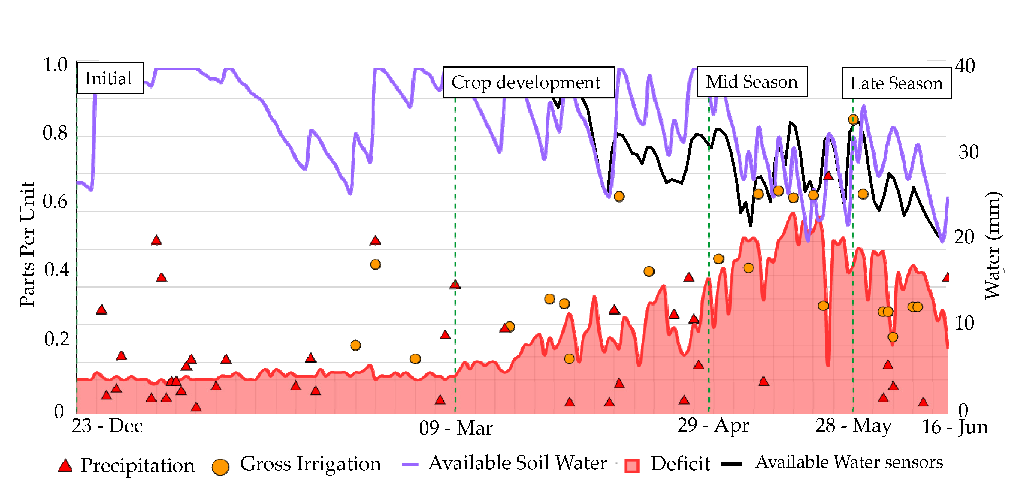
3.4. Irrigation Scheduling

During 2020, the gross irrigation water applied by farmers varied significantly, ranging from 187 mm for AVE 2 to 292 mm for LEA (Table 6). Nevertheless, despite most of the farmers supplying more irrigation water than that required by the crop, the ETa did not reach ETm, except in the case of LEA, which implies the crop suffered a deficit in certain stages of the cycle. This effect was simulated by the MOPECO irrigation scheduling tool (Figure 2), finding that it occurred when the available water (AW line) reached values below the allowable depletion level (1-p line). Evidently, the AW moves between wilting point (AW = 0) and field capacity (AW = 1).
Furthermore, LEA and AVE 1 farmers supplied an excess of irrigation water, which caused percolation (Table 6) in some periods. In these cases, the AW line reached and surpassed the field capacity level (Figure 2b,c). Nevertheless, in this year, the greater percolation was caused by the rainfall period that occurred at the end of March, and the non-efficient management of soil moisture, which caused great percolation of rainfall due to farmers keeping soil water content too high during the irrigation season. According to MOPECO, LEA generated the highest total percolation in 2020. This farmer aimed to maintain the soil moisture content very high (Figure 2b) as a way to decrease the impact on the yield of a potential lack of water availability at the end of the irrigation season in the irrigators’ community, as had occurred in previous seasons. However, SUP, using MOPECO to manage the irrigation of one subplot located in the LEA plot and under similar conditions, decreased the amount of percolated water by 38% with respect to this farmer, obtaining the lowest total percolation in the first year (Table 6). SUP reached a slightly lower ETa/ETm ratio than LEA at the end of the season. This difference was due to the deficit generated at the end of the growing season, as a way to increase the use of the soil moisture during a less sensitive stage to water deficit (ripening) of the crop [63,64]. AVE 2 (Figure 2d) applied the lowest amount of irrigation water, thanks to good irrigation water management and deeper soil, which allowed a greater amount of rainfall water to be stored than in the other plots under study.
Maintaining the soil moisture content excessively high in some periods does not mean farmers may not have caused deficits in other periods. AVE 3 (Figure 2e), for example, caused a deficit during highly sensitive stages related to the formation and filling of the grain [63,65,66]. Consequently, this farmer decreased the efficiency in the use of water in two ways: at the beginning of the irrigation season, by keeping the soil moisture content too high, favoring rainfall percolation; and during mid- and late seasons, by causing water stress to the crop in very sensitive stages. AVE 1 also caused a slight deficit during grain filling (Figure 2c).
In 2021, the leader farmer was trained in the use of the MOPECO irrigation scheduling tool and the methodologies proposed by SUPROMED, using them to manage another barley plot (LEASUP). That year, irrigation requirements increased 88 mm due to a decrease in the amount of rainfall received by the crop (Table 6). However, precipitation distribution was more homogeneous during the growing cycle and a lower percentage of rainfall should have caused percolation (Figure 3). LEASUP thus decreased the amount of percolated water by 45% compared to 2020 for a similar amount of irrigation water supplied to the crop. However, percolation could have been lower if rainfall forecasts had been more accurate, with some rainfall events being more substantial than predicted. Therefore, the farmer was able to fulfill the irrigation requirements of the crop (ETa/ETm = 1), decreasing percolation by using the soil moisture in a more suitable way.

3.5. Soil Water Monitoring

The evolution of available water in SUP (2020), LEA (2020), and LEASUP (2021) plots simulated by MOPECO tool presented a suitable goodness of fit in comparison to the real volumetric soil moisture measurements obtained by the probes, which were translated into available water. Figure 3 shows the available water progression in the LEASUP treatment, corroborating the better management of the irrigation water carried out by the Leader farmer when using the MOPECO tool during the second year in comparison to the management implemented in Year 1 (Table 6 and Figure 2b). Moreover, it can be stated that the soil water balance calculated by the model was properly calibrated for this crop in the area by [38].
The information provided by the pressure transducers and the soil moisture sensors allowed the SUPROMED team to corroborate the irrigation scheduling provided by the MOPECO irrigation scheduling tool, as well as to confirm the periods when the tool simulated percolation in the SUP, LEA, and LEASUP plots.

3.6. Analysis of the Key Performance Indicators

In both years, all the management types that did not suffer significant water deficits (Table 6) achieved similar yields and just above the calibrated potential value in the area (9000 kg ha−1 [38]) except AVE 1, which was a little lower (Table 7). The possible cause of this latter result was the lower amount of fertilizer (N and K) applied with respect to the calculated values [64,65,67] (Table 4), as well as the slight water deficit caused during the grain filling (Figure 2c). In contrast, the excessive amount of nitrogen fertilizers supplied by AVE 2 and AVE 3 did not increase the final yield compared to the other farmers. The great water deficit period caused in the AVE 3 plot (Figure 2e), as well as the low uniformity of the irrigation system (Table 2), justifies the drop in yield on this farm [63,65]. Despite LEA applying a lower number of fertilizer units than SUP, both achieved similar yields. The possible factors leading to LEA accomplishing a similar crop yield to that of SUP can be explained by considering that the crop extracted the difference from the soil nutrient pool. As discussed, the possible factors leading to AVE 2 achieving a similar crop yield to that of SUP, with 6% less irrigation water applied, can be explained by the soil being 25% deeper, the previous crop (maize for AVE 2 and garlic for SUP), and a higher nitrogen application, which increased grain number per unit area in conditions with higher water availability [67]. Yield values are similar to those obtained by [37,38,68], but slightly higher than [69] in the same study area and in other areas of Spain [67].
The different fertilizer and irrigation management types conditioned the nitrogen productivity (APN) in terms of yield. Thus, SUP was the plot that reached the highest APN in 2020, improving the result obtained by AVE 3 by 151%. As expected, SUP reached high WPC and WPI values, being surpassed only by AVE 2, due to the deeper soil characteristics on this farm. The improvement in WPI was mainly achieved by the more efficient use of soil moisture content, which reduced the percolation of rainfall water, while the improvement of WPC was due to avoiding water deficit during highly sensitive phenological stages (Table 6). Therefore, for an efficient use of water in areas where resources are scarce, it is as important to determine the irrigation requirements of the crop for each irrigation event as it is to establish the irrigation depth that allows the soil moisture content to be maintained within a range able to avoid water deficit between irrigations. It is also essential to store as much rainfall as possible; that is, if such rainfall occurs.
SUP had slightly lower total costs (lower use of fertilizers and irrigation water) and achieved a higher income per hectare than LEA, also thanks to a slightly higher yield (Table 7). Although the income obtained by AVE 1 and AVE 2 was similar to that of SUP and LEA, those farmers did not apply pest and disease treatments (around 10% of the total cost), thereby decreasing the total costs of barley cultivation on their farm and increasing the final gross margin (Table 7). AVE 3 obtained the worst economic values as a result of achieving the lowest yield in combination with high fertilization and irrigation costs (Table 4, Table 6 and Table 7). As expected, the economic productivity water indicators were more favorable for AVE 1 and AVE 2, thanks to cost savings. Nevertheless, SUP obtained better results than LEA and AVE 3, being very similar to those obtained by AVE 1. In comparison with other research, [68] achieved similar GM but much lower GEWPI compared to SUP in the same study area, receiving 37% less rainfall.
The WFTotal ranged between 0.43 m3kg−1 (SUP) and 0.59 m3kg−1 (AVE 3) (Table 7). SUP reached the most sustainable values, achieving the highest WFgreen, and the lowest WFblue, WFgrey and WFTotal (Table 7). Climatic conditions greatly affect WFgreen. In areas with low rainfall, irrigation supplies most of the crop water requirements, which involves the use of energy for pumping water from freshwater bodies to the farms and to the plots. Consequently, increasing WFgreen should decrease the use of energy on farms and the extraction of freshwater from rivers and aquifers, thus reducing WFblue. Moreover, a higher use of green water in combination with proper irrigation scheduling leads to lower percolation, which means lower transportation of dissolved fertilizers and pesticides to deeper soil areas, which may contaminate groundwater resources. In this way, the amount of fertilizer applied to the crop also affects WFgrey. The analytical determination of the nitrogen requirements for barley in the SUP subplot in combination with low percolation achieved the lowest WFgrey value.
In 2021, LEASUP improved almost all the indicators compared to LEA 2020. This was due to a 40% increase in the sale price of barley grain, a reduction in the application of pest and disease treatments, better management of the irrigation system, and a reduction in the use of fertilizers (Table 4). Thus, the farmer achieved higher profitability (172%) and a higher yield (6%), applied less irrigation water (2%), decreased the percolation (45%), and reduced the water footprint (4%).
The values obtained are in the line with the results obtained by [38] in the same area. Ref. [70] determined average CLM values of the three water footprint components for barley. For WFgreen, these authors reported a value of 1.21 m3 kg−1, which is significantly higher than the values obtained for all our management types. Additionally, they found a WFblue value of 0.08 m3 kg−1, which is lower than the values obtained in this study. Finally, a value of 0.13 m3 kg−1 for WFgrey was reported, which is significantly higher than those obtained by almost all of the management types in this study (Table 7). The differences can be justified by the study area, since the values obtained by [38] in the same area as in this study are very similar for all components.
The results obtained by the SUPROMED research team and LEASUP might have been even better had we used remote sensing tools included in the platform that allow water and nutritional crop requirements to be determined [71,72]. However, the image processing needs to be carried out by experts, who also have to interpret the results. Consequently, this is a service that must be paid for by end-users with sufficient economic capacity, which is not common in the Mediterranean basin. Consequently, this work only shows the impact on the management of farms of the models and methodologies in the platform that are free and can be directly applied by any type of farmer.

4. Conclusions

Despite the great professionalism of farmers, the lack of tools and methodologies adapted to their training and necessities negatively affects the profitability and sustainability of farms. Thus, the management of a barley crop based on the tools and methodologies adapted to farmers included in the SUPROMED platform improved most of the productive, economic, and environmental indicators calculated during the first-year monitoring of four traditional farms. This result was corroborated in the second year of the experiment, when a farmer (LEASUP) trained in the use of these methodologies improved all the key performance indicators with respect to the values obtained in Year 1 on his farm (LEA). Therefore, the models and methodologies proposed by SUPROMED demonstrated how the efficient use of inputs increases the profitability of farms and reduces the impact on the environment.
The use of the MOPECO irrigation scheduling tool, in combination with simple methodologies such as the use of pressure transducers and/or flowmeters, pluviometers installed on the farm, and the periodic evaluation of the irrigation systems, may allow farmers to improve the yield and economic productivity of irrigation water. In this way, it is possible to establish a more efficient use of precipitation water through better use of soil moisture. Moreover, the tool provides farmers with information about excessive or insufficient irrigation doses, which may cause water percolation or stress in the crop due to water deficit. To determine the irrigation scheduling, the MOPECO tool requires calibration for the crops in the area and access to the data registered by a local agrometeorological weather station.
Additionally, the use of soil analysis, in combination with the determination of the nutrients extracted by the crops during the growing season, may decrease the use of fertilizers and/or increase yields, affecting, in both cases, the environmental impact of the farm and the final income perceived by the farmer.
The positive results obtained by the farmer in the second monitoring year showed that the methodologies and tools in the platform were properly adapted to the training and requirements of the farmers, who can use them under real management conditions.
In consequence, the widespread use of the techniques and tools proposed by SUPROMED would help improve the economic and environmental sustainability of Mediterranean agroecosystems through more efficient management of water, energy, and fertilizers. To achieve this objective, the involvement of public administrations is necessary, in order to develop a network of weather stations in the main irrigable areas of their respective countries, to encourage local research teams to implement the models in the main irrigable areas by providing the validated parameters required by these tools, to train public and/or private technicians in the use of the models and methodologies to advise farmers in the management of their farms, and to organize training courses for farmers that show the positive impact of using these methodologies on the economic and environmental sustainability of their farms.

Author Contributions

Conceptualization, A.D. and R.L.-U.; methodology, R.L.-U., A.D. and J.J.P.; software, Á.M.-R. and A.D.; validation, J.A.M.-L. and J.J.P.; formal analysis, J.A.M.-L., J.J.P., R.L.-U. and A.D.; investigation, J.A.M.-L., J.J.P. and J.M. and A.D.; resources, A.D. and R.L.-U.; data curation, J.A.M.-L. and J.J.P.; writing—original draft preparation, J.A.M.-L.; writing—review and editing, J.A.M.-L., J.J.P., Á.M.-R., R.L.-U., J.M. and A.D.; visualization, R.L.-U. and A.D.; supervision, R.L.-U. and A.D.; project administration, A.D.; funding acquisition, A.D. and R.L.-U. All authors have read and agreed to the published version of the manuscript.

Funding

This research was carried out under the framework of European project SUPROMED “GA-1813” funded by PRIMA, and the Regional project PRODAGUA “Ref SBPLY/19/180501/000144” funded by FEDER and the Regional Government of Castilla-La Mancha.

Institutional Review Board Statement

Not applicable.

Informed Consent Statement

Not applicable.

Acknowledgments

The authors thank the farmers participating in this research for their support in implementing the tasks and actions carried out over the two monitoring years.

Conflicts of Interest

The authors declare no conflict of interest. The funders had no role in the design of the study; in the collection, analyses, or interpretation of data; in the writing of the manuscript, or in the decision to publish the results.

References

  1. García-Ruiz, J.M.; López-Moreno, J.I.; Vicente-Serrano, S.M.; Lasanta–Martínez, T.; Beguería, S. Mediterranean Water Resources in a Global Change Scenario. Earth-Sci. Rev. 2011, 105, 121–139. [Google Scholar] [CrossRef] [Green Version]
  2. Correia, F.N.; Iwra, M.; Técnico, I.S. Water Resources in the Mediterranean Region. Int. Water Resour. Assoc. 2009, 24, 22–30. [Google Scholar] [CrossRef]
  3. De Juan, J.A.; Tarjuelo, J.M.; Valiente, M.; García, P. Model for Optimal Cropping Patterns within the Farm Based on Crop Water Production Functions and Irrigation Uniformity. I: Development of a Decision Model. Agric. Water Manag. 1996, 31, 115–143. [Google Scholar] [CrossRef]
  4. Nascimento, A.K.; Schwartz, R.C.; Lima, F.A.; López-Mata, E.; Domínguez, A.; Izquiel, A.; Tarjuelo, J.M.; Martínez-Romero, A. Effects of Irrigation Uniformity on Yield Response and Production Economics of Maize in a Semiarid Zone. Agric. Water Manag. 2019, 211, 178–189. [Google Scholar] [CrossRef]
  5. López-Mata, E.; Tarjuelo, J.M.; de Juan, J.A.; Ballesteros, R.; Domínguez, A. Effect of Irrigation Uniformity on the Profitability of Crops. Agric. Water Manag. 2010, 98, 190–198. [Google Scholar] [CrossRef]
  6. Daccache, A.; Ciurana, J.S.; Rodríguez Díaz, J.A.; Knox, J.W. Water and Energy Footprint of Irrigated agriculture in the Mediterranean Region. Environ. Res. Lett. 2014, 9, 124014. [Google Scholar] [CrossRef]
  7. Knox, J.; Hess, T.; Daccache, A.; Wheeler, T. Climate Change Impacts on Crop Productivity in Africa and South Asia. Environ. Res. Lett. 2012, 7, 034032. [Google Scholar] [CrossRef]
  8. Tarjuelo, J.M.; Rodriguez-Diaz, J.A.; Abadía, R.; Camacho, E.; Rocamora, C.; Moreno, M.A. Efficient Water and Energy Use in Irrigation Modernization: Lessons from Spanish Case Studies. Agric. Water Manag. 2015, 162, 67–77. [Google Scholar] [CrossRef]
  9. Sachalkoff, R.J. Artificial Neural Networks; McGraw Hill: New York, NY, USA, 1997. [Google Scholar]
  10. Hill, T.R.; Marquez, L.; O’Connor, M.; Remus, W. Artificial Neural Network Models for Forecasting and Decision Making. Int. J. Forecast. 1994, 10, 5–15. [Google Scholar] [CrossRef] [Green Version]
  11. Suzuki, J.; Ueno, M. Advanced Methodologies for Bayesian Networks. In Proceedings of the Second International Workshop, AMBN 2015, Yokohama, Japan, 16–18 November 2015; Volume 9505, ISBN 978-3-319-28378-4. [Google Scholar]
  12. Hernández, L.; Baladrón, C.; Aguiar, J.M.; Calavia, L.; Carro, B.B.; Sánchez-Esguevillas, A.; Pérez, F.; Fernández, Á.; Lloret, J. Artificial Neural Network for Short-Term Load Forecasting in Distribution Systems. Energies 2014, 7, 1576–1598. [Google Scholar] [CrossRef] [Green Version]
  13. Yao, J.; Meng, D.; Zhao, Q.; Cao, W.; Xu, Z. Nonconvex-Sparsity and Nonlocal-Smoothness-Based Blind Hyperspectral Unmixing. IEEE Trans. Image Process. 2019, 28, 2991–3006. [Google Scholar] [CrossRef] [PubMed]
  14. Du, C.; Tang, D.; Zhou, J.; Wang, H.; Shaviv, A. Prediction of Nitrate Release from Polymer-Coated Fertilizers Using an Artificial Neural Network Model. Biosyst. Eng. 2008, 99, 478–486. [Google Scholar] [CrossRef]
  15. Vlontzos, G.; Pardalos, P.M. Assess and Prognosticate Green House Gas Emissions from Agricultural Production of EU Countries, by Implementing, DEA Window Analysis and Artificial Neural Networks. Renew. Sustain. Energy Rev. 2017, 76, 155–162. [Google Scholar] [CrossRef]
  16. Pereira, L.S.; Teodoro, P.R.; Rodrigues, P.N.; Teixeira, J.L. Irrigation Scheduling Simulation: The Model ISAREG. In Tools for Drought Mitigation in Mediterranean Regions; Springer: Dordrecht, The Netherlands, 2003; pp. 161–180. [Google Scholar]
  17. Stockle, C.; Donatelli, M.; Nelson, R. CropSyst, a Cropping Systems Simulation Model. Eur. J. Agron. 2003, 18, 289–307. [Google Scholar] [CrossRef]
  18. Van Dam, J.C.; Huygen, J.; Wesseling, J.G.; Feddes, R.A.; Kabat, P.; Van, P.E.V.; Groenendijk, W.P.; Van, C.A.; Report, D. Theory of SWAP Version 2.0: Simulation of Water Flow, Solute Transport and Plant Growth in the Soil-Water-Atmosphere-Plant Environment; DLO Winand Staring Centre: Wageningen, The Netherlands, 1997. [Google Scholar]
  19. Vanuytrecht, E.; Raes, D.; Steduto, P.; Hsiao, T.C.; Fereres, E.; Heng, L.K.; Garcia Vila, M.; Mejias Moreno, P. AquaCrop: FAO’s Crop Water Productivity and Yield Response Model. Environ. Model. Softw. 2014, 62, 351–360. [Google Scholar] [CrossRef]
  20. Ortega Álvarez, J.F.; de Juan Valero, J.A.; Tarjuelo Martín-Benito, J.M.; López Mata, E. MOPECO: An Economic Optimization Model for Irrigation Water Management. Irrig. Sci. 2004, 23, 61–75. [Google Scholar] [CrossRef]
  21. Domínguez, A.; de Juan, J.A.; Tarjuelo, J.M.; Martínez, R.S.; Martínez-Romero, A. Determination of Optimal Regulated Deficit Irrigation Strategies for Maize in a Semi-Arid Environment. Agric. Water Manag. 2012, 110, 67–77. [Google Scholar] [CrossRef]
  22. Domínguez, A.; Tarjuelo, J.M.; de Juan, J.A.; López-Mata, E.; Breidy, J.; Karam, F. Deficit Irrigation under Water Stress and Salinity Conditions: The MOPECO-Salt Model. Agric. Water Manag. 2011, 98, 1451–1461. [Google Scholar] [CrossRef]
  23. Domínguez, A.; Martínez, R.S.; de Juan, J.A.; Martínez-Romero, A.; Tarjuelo, J.M. Simulation of Maize Crop Behavior under Deficit Irrigation Using MOPECO Model in a Semi-Arid Environment. Agric. Water Manag. 2012, 107, 42–53. [Google Scholar] [CrossRef]
  24. Domínguez, A.; Schwartz, R.C.; Pardo, J.J.; Guerrero, B.; Bell, J.M.; Colaizzi, P.D.; Louis Baumhardt, R. Center Pivot Irrigation Capacity Effects on Maize Yield and Profitability in the Texas High Plains. Agric. Water Manag. 2022, 261, 107335. [Google Scholar] [CrossRef]
  25. Domínguez, A.; Jiménez, M.; Tarjuelo, J.M.; de Juan, J.A.; Martínez-Romero, A.; Leite, K.N. Simulation of Onion Crop Behavior under Optimized Regulated Deficit Irrigation Using MOPECO Model in a Semi-Arid Environment. Agric. Water Manag. 2012, 113, 64–75. [Google Scholar] [CrossRef]
  26. Domínguez, A.; Martínez-Romero, A.; Leite, K.N.; Tarjuelo, J.M.; de Juan, J.A.; López-Urrea, R. Combination of Typical Meteorological Year with Regulated Deficit Irrigation to Improve the Profitability of Garlic Growing in Central Spain. Agric. Water Manag. 2013, 130, 154–167. [Google Scholar] [CrossRef]
  27. Leite, K.N.; Cabello, M.J.; Valnir, M., Jr.; Tarjuelo, J.M.; Domínguez, A. Modelling Sustainable Salt Water Management under Deficit Irrigation Conditions for Melon in Spain and Brazil. J. Sci. Food Agric. 2015, 95, 2307–2318. [Google Scholar] [CrossRef] [PubMed]
  28. Carvalho, D.F.; Domínguez, A.; Neto, D.H.O.; Tarjuelo, J.M.; Martínez-Romero, A. Combination of Sowing Date with Deficit Irrigation for Improving the Profitability of Carrot in a Tropical Environment (Brazil). Sci. Hortic. 2014, 179, 112–121. [Google Scholar] [CrossRef]
  29. Léllis, B.C.; Carvalho, D.F.; Martínez-Romero, A.; Tarjuelo, J.M.; Domínguez, A. Effective Management of Irrigation Water for Carrot under Constant and Optimized Regulated Deficit Irrigation in Brazil. Agric. Water Manag. 2017, 192, 294–305. [Google Scholar] [CrossRef]
  30. Martínez-Romero, A.; Domínguez, A.; Landeras, G. Regulated Deficit Irrigation Strategies for Different Potato Cultivars under Continental Mediterranean-Atlantic Conditions. Agric. Water Manag. 2019, 216, 164–176. [Google Scholar] [CrossRef]
  31. Carrión, F.; Sanchez-Vizcaino, J.; Corcoles, J.I.; Tarjuelo, J.M.; Moreno, M.A. Optimization of Groundwater Abstraction System and Distribution Pipe in Pressurized Irrigation Systems for Minimum Cost. Irrig. Sci. 2016, 34, 145–159. [Google Scholar] [CrossRef]
  32. Merriam, J.L.; Keller, J. Farm Irrigation System Evaluation: A Guide for Management; Utah State University: Logan, UT, USA, 1978. [Google Scholar]
  33. ASAE. ASAE.S 330.1. Procedure for Sprinkler Distribution Testing for Research Purposes. In ASAE Standards; ASAE, Ed.; ASAE: St. Joseph, MI, USA, 1985. [Google Scholar]
  34. ISO 1145:2009; Agricultural Irrigation Equipment-Centre-Pivot and Moving Lateral Irrigation Machines with Sprayer or Sprinkler Nozzles-Determination of Uniformity of Water Distribution. 3rd edition. ISO: Geneva, Switzerland, 2009.
  35. Allen, R.G.; Pereira, L.S.; Raes, D.; Smith, M. Crop Evapotranspiration-Guidelines for Computing Crop Water Requirements—FAO Irrigation and Drainage Paper 56; FAO: Rome, Italy, 1998. [Google Scholar]
  36. Rodriguez-Diaz, J.A.; Camacho-Poyato, E.; Carrillo-Cobo, M.T. The Role of Energy Audits in Irrigated Areas. The Case of ‘Fuente Palmera’ Irrigation District (Spain). Span. J. Agric. Res. 2010, 8, 152. [Google Scholar] [CrossRef] [Green Version]
  37. Martínez-Romero, A.; Martínez-Navarro, A.; Pardo, J.J.; Montoya, F.; Domínguez, A. Real Farm Management Depending on the Available Volume of Irrigation Water (Part II): Analysis of Crop Parameters and Harvest Quality. Agric. Water Manag. 2017, 192, 58–70. [Google Scholar] [CrossRef]
  38. Pardo, J.J.; Martínez-Romero, A.; Léllis, B.C.; Tarjuelo, J.M.; Domínguez, A. Effect of the Optimized Regulated Deficit Irrigation Methodology on Water Use in Barley under Semiarid Conditions. Agric. Water Manag. 2020, 228, 105925. [Google Scholar] [CrossRef]
  39. Léllis, B.C.; Martínez-Romero, A.; Schwartz, R.C.; Pardo, J.J.; Tarjuelo, J.M.; Domínguez, A. Effect of the Optimized Regulated Deficit Irrigation Methodology on Water Use in Garlic. Agric. Water Manag. 2022, 260, 107280. [Google Scholar] [CrossRef]
  40. FAOSTAT. Food and Agriculture Organization of the United Nations, Rome, Italy. Available online: https://www.fao.org/faostat/en/#data (accessed on 7 February 2022).
  41. MAPA. Avance de Datos de Cereales Año. 2020. Available online: https://www.mapa.gob.es/es/estadistica/temas/estadisticas-agrarias/agricultura/superficies-producciones-anuales-cultivos/ (accessed on 7 February 2022).
  42. Papadakis, J. Climates of the World and Their Agricultural Potentialities; Hemisferio Sur: Buenos Aires, Argentina, 1966. [Google Scholar]
  43. United States Department of Agriculture; Natural Resources Conservation Services. Keys to Soil Taxonomy, 10th ed.; United States Department of Agriculture: Washington, DC, USA, 2006.
  44. Pereira, L.S.; Paredes, P.; Hunsaker, D.J.; López-Urrea, R.; Mohammadi Shad, Z. Standard Single and Basal Crop Coefficients for Field Crops. Updates and Advances to the FAO56 Crop Water Requirements Method. Agric. Water Manag. 2021, 243, 106196. [Google Scholar] [CrossRef]
  45. Bleiholder, H.; Weber, E.; Lancashire, P.D.; Feller, C.; Buhr, L.; Hess, M.; Wicke, H.; Hack, H.; Meier, U.; Klose, R.; et al. Growth Stages of Mono- and Dicotyledonous Plants BBCH Monograph, 2nd ed.; Meier, U., Ed.; Federal Biological Research Centre for Agriculture and Forestry: Braunschweig, Germany, 2001. [Google Scholar]
  46. Danuso, F.; Gani, M.; Giovanardi, R. Field Water Balance: BidriCo 2. In Crop-Water Simulation Model in Practice. ICI-CIID, SC-DLO; Pereira, L.S., van der Broeck, B.J., Kabat, P., Allen, R.G., Eds.; Wageningen Press: Wageningen, The Netherlands, 1995. [Google Scholar]
  47. Agencia Estatal de Meteorología. Gobierno de España. Available online: http://www.aemet.es/es/portada (accessed on 3 May 2022).
  48. Trigo, I.F.; de Bruin, H.; Beyrich, F.; Bosveld, F.C.; Gavilán, P.; Groh, J.; López-Urrea, R. Validation of Reference Evapotranspiration from Meteosat Second Generation (MSG) Observations. Agric. For. Meteorol. 2018, 259, 271–285. [Google Scholar] [CrossRef]
  49. López-Urrea, R.; Pardo, J.J.; Simón, L.; Martínez-Romero, Á.; Montoya, F.; Tarjuelo, J.M.; Domínguez, A. Assessing a Removable Mini-Lysimeter for Monitoring Crop Evapotranspiration Using a Well-Established Large Weighing Lysimeter: A Case Study for Barley and Potato. Agronomy 2021, 11, 2067. [Google Scholar] [CrossRef]
  50. United States Department of Agriculture. SCS Section 4: Hidrology. In National Engineering Handbook; Soil Conservation Service, Ed.; United States Department of Agriculture: Washington, DC, USA, 1972. [Google Scholar]
  51. United States Department of Agriculture. NRCS Estimation of Direct Runoff from Storm Rainfall. In National Engineering Handbook; Natural Resources Conservation Service, Ed.; United States Department of Agriculture: Washington, DC, USA, 2004. [Google Scholar]
  52. Westfall, P.H.; Young, S.S. Resampling-Based Multiple Testing: Examples and Methods for p-Value Adjustment; John Wiley & Sons: Hoboken, NJ, USA, 1993; Volume 279, p. 340. [Google Scholar]
  53. Fernández, J.E.; Alcon, F.; Diaz-Espejo, A.; Hernandez-Santana, V.; Cuevas, M.V. Water Use Indicators and Economic Analysis for On-Farm Irrigation Decision: A Case Study of a Super High Density Olive Tree Orchard. Agric. Water Manag. 2020, 237, 106074. [Google Scholar] [CrossRef]
  54. Hoekstra, A.Y.; Chapagain, A.K.; Aldaya, M.M.; Mekonnen, M.M. Water Footprint Manual: State of the Art 2009; Water Footprint Network: Enschede, The Netherlands, 2009; 127p. [Google Scholar]
  55. European Union. CEE, 1991. Directive 91/676/CEE; European Union: Brussels, Belgium, 1991. [Google Scholar]
  56. Franke, N.; Hoekstra, A.Y.; Boyacioglu, H. Grey Water Footprint Accounting: Tier 1 Supporting Guidelines; Value of Water Research Report Series, 65; UNESCO-IHE: Delf, The Netherlands, 2013; pp. 343–354. [Google Scholar]
  57. Ministerio de Agricultura, Pesca y Alimentacion. Informe Semanal de Coyuntura. Available online: https://www.mapa.gob.es/es/estadistica/temas/publicaciones/informe-semanal-coyuntura/2020.aspx (accessed on 23 June 2020).
  58. Ministerio de Agricultura, Pesca y Alimentacion. Informe Semanal de Coyuntura. Available online: https://www.mapa.gob.es/es/estadistica/temas/publicaciones/informesemanaldecoyunturas-31_tcm30-573276.pdf (accessed on 3 August 2021).
  59. CHJ. Confederacion Hidrográfica del Jucar Estado Químico Anual. Informes del Programa de Control de Vigilancia de Aguas Subterráneas. 2017. Available online: https://www.chj.es/es-es/medioambiente/redescontrol/InformesAguasSubterraneas/Estado%20Qu%C3%ADmico%20anual%202017.pdf (accessed on 10 February 2022).
  60. Domínguez Vivancos, A. Tratado de Fertilizacion; Mundi-Prensa: Madrid, Spain, 1989. [Google Scholar]
  61. Boyeldiu, J. Les Cultures Céréaliéres; Hachette: Paris, France, 1980. [Google Scholar]
  62. Sevacherian, V.; Stern, V.M.; Mueller, A.J. Heat Accumulation for Timing Lygus Control Measures in a Safflower-Cotton Complex 2. J. Econ. Entomol. 1977, 70, 399–402. [Google Scholar] [CrossRef]
  63. Abrha, B.; Delbecque, N.; Raes, D.; Tsegay, A.; Todorovic, M.; Heng, L.E.E.; Vanutrecht, E.; Geerts, S.A.M.; Garcia-Vila, M.; Deckers, S. Sowing Strategies for Barley (Hordeum vulgare L.) Based on Modelled Yield Response to Water with Aquacrop. Exp. Agric. 2012, 48, 252–271. [Google Scholar] [CrossRef] [Green Version]
  64. Al Azzawi, W.; Gill, M.B.; Fatehi, F.; Zhou, M.; Acuña, T.; Shabala, L.; Yu, M.; Shabala, S. Effects of Potassium Availability on Growth and Development of Barley Cultivars. Agronomy 2021, 11, 2269. [Google Scholar] [CrossRef]
  65. Cossani, C.M.; Slafer, G.A.; Savin, R. Yield and Biomass in Wheat and Barley under a Range of Conditions in a Mediterranean Site. Field Crops Res. 2009, 112, 205–213. [Google Scholar] [CrossRef]
  66. Arisnabarreta, S.; Miralles, D.J. Critical Period for Grain Number Establishment of near Isogenic Lines of Two- and Six-Rowed Barley. Field Crops Res. 2008, 107, 196–202. [Google Scholar] [CrossRef]
  67. Cossani, C.M.; Slafer, G.A.; Savin, R. Nitrogen and Water Use Efficiencies of Wheat and Barley under a Mediterranean Environment in Catalonia. Field Crops Res. 2012, 128, 109–118. [Google Scholar] [CrossRef]
  68. Domínguez, A.; Martínez-Navarro, A.; López-Mata, E.; Tarjuelo, J.M.; Martínez-Romero, A. Real Farm Management Depending on the Available Volume of Irrigation Water (Part I): Financial Analysis. Agric. Water Manag. 2017, 192, 71–84. [Google Scholar] [CrossRef]
  69. López-Urrea, R.; Domínguez, A.; Pardo, J.J.; Montoya, F.; García-Vila, M.; Martínez-Romero, A. Parameterization and Comparison of the AquaCrop and MOPECO Models for a High-Yielding Barley Cultivar under Different Irrigation Levels. Agric. Water Manag. 2020, 230, 105931. [Google Scholar] [CrossRef]
  70. Mekonnen, M.M.; Hoekstra, A.Y. The Green, Blue and Grey Water Footprint of Crops and Derived Crops Products; Value of Water Research Report Series No. 47; UNESCO-IHE: Delf, The Netherlands, 2010. [Google Scholar]
  71. Dalezios, N.R.; Faraslis, I.N. Remote Sensing in Agricultural Production Assessment. Modeling for Sustainable Management in Agriculture, Food and the Environment; CRC Press: Boca Raton, FL, USA, 2021; pp. 172–198. [Google Scholar] [CrossRef]
  72. Skamarock, W.C.; Klemp, J.B.; Dudhia, J.; Gill, D.O.; Barker, D.M.; Wang, W.; Powers, J.G. A Description of the Advanced Research WRF Version 3; NCAR Technical 15 Note NCAR/TN—475 + STR; National Center for Atmospheric Research: Boulder, CO, USA, 2008; p. 113. [Google Scholar]
Figure 1. Location of the monitored area in southeastern Spain. HUEM: hydrogeological unit of eastern Mancha.
Agronomy 12 01358 g001
Figure 2. Evolution of available water simulated by “MOPECO irrigation scheduling” tool in 2020 (a): SUP, SUP: Supromed management; (b) LEA: Leader management; (ce): AVE: Average management. Main Y axis: deficit: 1-p, where p is the fraction of total available water (TAW) that a crop can extract without suffering water stress; available water. Secondary Y axis: gross irrigation; precipitation.
Agronomy 12 01358 g002
Figure 3. Evolution of available soil water (AW; main Y axis) simulated by online MOPECO model for LEADER using SUPROMED tool (LEASUP) in 2021 and comparison with measured (Drill & Drop, Senteck) available soil moisture progression in LEASUP (2021) (available water sensors; main Y axis). Where deficit (main Y axis): 1-p, where p is the fraction of total available water (TAW) that a crop can extract without suffering from water stress. Secondary Y axis: gross irrigation; precipitation.
Agronomy 12 01358 g003
Table 1. Monitored barley plots.
YearCrop ManagementSurface (ha)Sowing DateHarvest Date
2020SUP2.9318 December 201919 June 2020
LEA7.8518 December 201919 June 2020
AVE 14.804 December 201910 June 2020
AVE 215.9515 January 201919 June 2020
AVE 342.6730 January 201929 June 2020
2021 LEASUP4.6523 December 202016 June 2021
Where: SUP: Supromed; LEA: Leader; AVE: Average; LEASUP: LEA using SUP platform.
Table 2. Characterization of monitored irrigation systems.
YearCrop ManagementSprinkler Spacing
(m × m)
Pressure
(kPa)
Sprinkler
Discharge
(L h−1)
Application Rate
(mm h−1)
DU
(%)
CU (%)
2020SUP17.3 × 17.3402.52052.66.975.785.9
LEA17.3 × 17.3358.81966.76.677.887.4
AVE 117.3 × 16.8366.42108.97.076.5 *86.7 *
AVE 217.3 × 17.3354.41962.66.676.5 *86.7 *
AVE 317.5 × 17.5403.02085.16.843.868.5
2021LEASUP 17.3 × 17.3403.82002.96.779.485.9
Where: SUP: Supromed; LEA: Leader; AVE: Average; LEASUP: LEA using SUP platform; DU: distribution uniformity; CU: Christiansen’s coefficient of uniformity; * Due to the lockdown imposed under the COVID-19 pandemic on March 15, these evaluations were not carried out. Estimated DU and CU values were included.
Table 3. Parameters required by MOPECO model to determine the irrigation scheduling of a barley crop under the climatic conditions in Castilla-La Mancha [38].
StageKcPhenological StageGDD (°C)Others ParametersValue
I0.300–21290.3ET group3
II0.30–1.1521–39744.5TL (°C)2
III1.1539–831087.2TU (°C)28
IV1.15–0.4583–891449.5
Kc: crop coefficient values used by the irrigation advisory service of CLM (SIAR) based on those proposed by FAO 56 and calibrated to the regional conditions; Kc (I): initial; Kc (II): crop development; Kc (III): mid-season; Kc (IV): late season [35,44]; 00: first day after sowing; 21: beginning of tillering: first tiller detectable; 39: flag leaf stage: flag leaf fully unrolled, ligule just visible; 83: early dough; 89: fully ripe: grain hard, difficult to divide with thumbnail [45]; GDD: cumulative growing degree day [38]; ET group: this conditions the daily value of the fraction of the total available water (TAW) that a crop can extract without suffering from water stress [46]; TU is the upper developmental threshold temperature or the temperature at and above which the rate of development begins to decrease [38]; TL is the lower developmental threshold temperature or the temperature at and below which development stops [38].
Table 4. Calculated and observed values of fertilizers.
Calculated Applied
N/P2O5/K2O
(kg ha−1)
Cost
(EUR ha−1)
N/P2O5/K2O
(kg ha−1)
Cost
(EUR ha−1)
SUP125/55/213301125/219/266336
LEA125/55/213301125/219/123264
AVE 1204/147/252435123/45/45210
AVE 2116/0/147175244/110/96181
AVE 3110/0/147169244/179/95298
LEASUP209/138/233342109/103/48156
SUP: Supromed management; LEA: Leader management; AVE: Average management; LEASUP: LEA using SUP platform.
Table 5. Observed CGDD and dates of the different growing stages for the two years of the trial.
Year Sowing DateHarvest DateGDD
2020SUP18-December19-June1566
LEA18-December19-June1566
AVE 104-December10-June1673
AVE 215-January19-June1514
AVE 330-January29-June1542
2021LEASUP23-December16-June1572
GDD: cumulative growing degree day [62] SUP: Supromed management; LEA: Leader management; AVE: Average management; LEASUP: LEA using SUP platform.
Table 6. Total water received by the crop and ETa/ETm ratio reached at the end of the crop cycle.
Ig (mm)In (mm)PI (mm)Re (mm)Pr (mm)In + Re (mm)ETa (mm)ETm (mm)ETa/ETm
SUP199.6159.70.0234.090.5393.6347.0355.20.98
LEA292.1233.719.4234.0125.2467.6355.2355.21.00
AVE 1222.7189.35.0236.9104.3426.2331.4334.60.99
AVE 2186.9158.80.0231.3106.0390.1338.0349.00.97
AVE 3240.9192.70.0194.7106.0387.4313.5346.50.92
LEASUP287.4229.919.3191.860.1421.7350.0353.01.00
Ig: gross irrigation; In: net Irrigation; PI: percolation due to irrigation events; Re: effective rainfall, Pr: rain percolation; In + Pe: net irrigation + effective precipitation; ETa: actual crop evapotranspiration; ETm: potential crop evapotranspiration.
Table 7. Grain yield and water productivity in the different management types in the two barley growing seasons.
Year20202021
Crop ManagementSUPLEAAVE 1AVE 2AVE 3LEASUP
Yield (kg ha−1)9467 a9295 a8776 ab9564 a7350 a9828
SD (kg)1446184910367451102929
Cv (%)15.319.911.87.815.09.5
APN (kg UFN−1)75.7474.3671.3539.2030.1290.17
WPc (kg m−3)2.732.622.652.832.342.81
WPI (kg m−3)4.743.183.945.123.053.42
Ct (EUR ha−1)1156.481195.50976.74865.201077.01958.81
Vp (EUR ha−1)1745.491718.871689.791760.511368.242383.19
GM (EUR ha−1)589.01523.37713.05895.31291.231424.38
GEWPI (EUR m−3)0.300.180.320.480.120.50
NEWP (EUR m−3)0.150.110.170.230.080.34
WFGreen (m3 kg −1)0.180.130.170.140.130.15
WFBlue (m3 kg −1)0.170.230.210.170.250.21
WFgrey (m3 kg −1)0.080.080.090.160.210.07
WFTotal (m3 kg −1)0.430.450.470.470.590.43
SD: standard deviation; CV: coefficient of variation; significance level (p < 0.05). Duncan’s test; APN: agronomic productivity of N; WPc: crop water productivity; WPI: irrigation water productivity.; Ct: total costs; Vp: total value of the commodity; GM: gross margin; GEWPI: gross economic irrigation water productivity; NEWP: net economic water productivity; WFGreen: green water footprint; WFBlue: blue water footprint; WFgrey: grey water footprint; WFTotal: total water footprint.
Publisher’s Note: MDPI stays neutral with regard to jurisdictional claims in published maps and institutional affiliations.

