Silage Grass Sward Nitrogen Concentration and Dry Matter Yield Estimation Using Deep Regression and RGB Images Captured by UAV

Abstract

Agricultural grasslands are globally important for food production, biodiversity, and greenhouse gas mitigation. Effective strategies to monitor grass sward properties, such as dry matter yield (DMY) and nitrogen concentration, are crucial when aiming to improve the sustainable use of grasslands in the context of food production. UAV-borne spectral imaging and traditional machine learning methods have already shown the potential to estimate DMY and nitrogen concentration for the grass swards. In this study, convolutional neural networks (CNN) were trained using low-cost RGB images, captured from a UAV, and agricultural reference measurements collected in an experimental grass field in Finland. Four different deep regression network architectures and three different optimizers were assessed. The best average results of the cross-validation were achieved by the VGG16 architecture with optimizer Adadelta: $r^2$ of 0.79 for DMY and $r^2$ of 0.73 for nitrogen concentration. The results demonstrate that this is a promising and effective tool for practical applications since the sensor is low-cost and the computational processing is not time-consuming in comparison to more complex sensors.

1. Introduction

Monitoring agricultural grassland fields is a crucial task for sustainable planning and resource management, which are essential features of climate change studies. Without efficiency and sustainable practices, the agriculture expansion can accumulate considerable environmental losses and biodiversity degradation [1]. Grasslands are becoming recognized as an extremely important ecosystem for food security, biodiversity conservation, maintenance of soil fertility, and greenhouse gas mitigation in terms of global carbon sequestration [2,3]. Although grasslands have a crucial role in the environment, the intensive use of the land can lead to negative environmental impacts. Effective and reliable information about the properties of forage (e.g., biomass and quality) is required, for instance, to choose suitable seed mixtures, fertilizer application rates, and the best time for harvesting. Grass silage plays an important role in ruminant meat and milk production in Northern Europe, focusing on food security and climate change [2]. Fresh and dry biomass and nitrogen are essential parameters for the management of quantity and quality management of swards. The most accurate way to collect information about above-ground biomass (i.e., yield for grass) is to cut and weigh a fresh sample of grass collected from a pre-defined size area. If the dry matter yield is also of interest, the sample is dried before measuring its weight. For the nitrogen concentration, the sample can be further sent to a laboratory for near-infrared spectroscopy analysis (NIRS; 800–2500 nm). However, these strategies are time-consuming and laborious, especially for large areas. Crop growth models can be used to simulate grass properties such as biomass, but typically they require extensive information about growing conditions, such as water dynamics and soil properties, as concluded by Korhonen et al. [4] in their study for Timothy grass conducted in Northern Europe and Canada. Satellite-based remote sensing has been used to estimate grass properties at large scales since the 1980s, but much less than for other crops, such as cereals, as reviewed by Reinermann et al. [5]. In previous years, unmanned aerial vehicles (UAV) have been bridging the gap between satellite and terrestrial approaches, providing a low-cost and flexible way to collect remote sensing data locally [6,7].

Previous studies showed the potential of combining UAV remote sensing and machine learning to estimate grassland parameters. Oliveira et al. [8], for example, investigated traditional machine learning methods (random forest and multiple linear regression) to estimate biomass and quality parameters. More accurate results were achieved when combining hyperspectral and 3D data from a crop height model. Unfortunately, hyperspectral sensors are not widespread due to their expensive cost, more complex and time-consuming data processing and analysis than sensors using less spectral bands. In this context, solutions based only on RGB sensors become interesting—for instance, for low cost and near- or real-time solutions, which reduces reproducibility opportunities.

Deep learning-based methods have surpassed traditional machine learning methods in many study cases [9]. Among various deep learning methods, convolutional neural networks (CNN) have been the most employed in agricultural applications based on UAV-driven remote sensing [10,11]. Yield estimation is an important task in agriculture, and CNN architectures based on UAV images have proven suitable for predicting the yields of various cereal crops, such as winter wheat [12], spring wheat, barley and oat [13], rice [14], corn [15] or strawberry [16] and citrus fruits [17]. However, studies where grass yield (above-ground biomass) is predicted using CNN-based methods are still rare. Castro et al. [18] combined deep learning and RGB data to estimate the green biomass of a pasture site in Brazil. CNNs, such as AlexNet, ResNet18 and VGGNet, were adapted for the regression task, and only the Adam optimization method was used. For the same study area, de Oliveira et al. [19] investigated CNNs to estimate dry matter yield and proposed their application in a guineagrass breeding program.

Nitrogen is the most important nutrient for grass growth and therefore has been widely used in the remote sensing literature, especially using laboratory and satellite-based approaches [20]. Drone-based remote sensing imagery has been utilized for nitrogen estimation, for instance, by Geipel et al. [21], Liu et al. [22], Näsi et al. [23] and Oliveira et al. [8], or for crude protein (strongly linked with nitrogen) as reported in Capolupo et al. [24], Askari et al. [25], Michez et al. [26] and Barnetson et al. [27]. However, to our knowledge, deep learning regression-based approaches for grass nitrogen prediction are even less explored than biomass estimations. As there are several CNN architectures and optimizers, it is important to investigate the optimal configurations for an application. The aim of this study was to assess the suitability of CNN-based approaches by comparing different deep regression network architectures (DenseNet201, InceptionV3, VGG16 and Xception) and optimizers (Adadelta, Adagrad and Adam) to estimate grass sward nitrogen concentration (N) and dry matter yield (DMY) using RGB images collected from a drone.

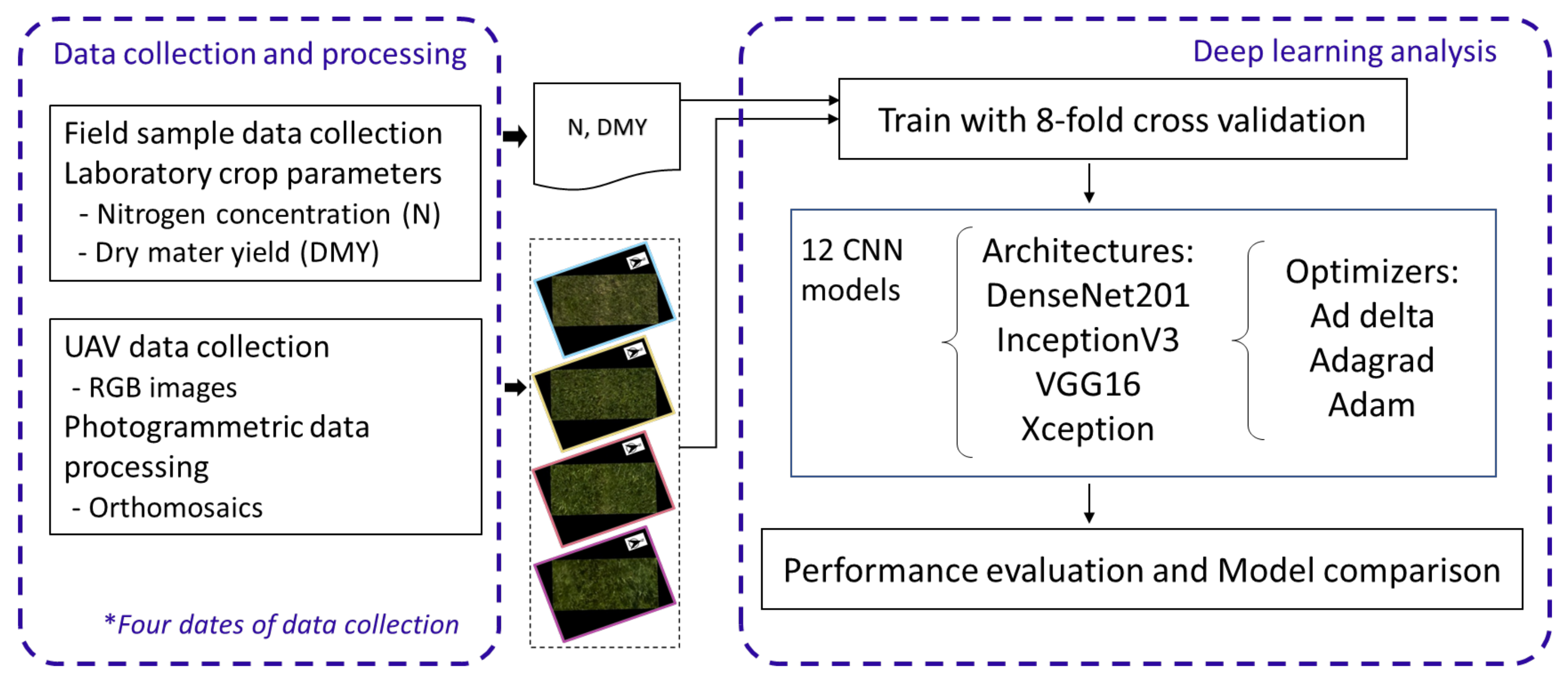
2. Materials and Methods

The workflow of this study included (1) grass sample collection and UAV remote sensing data collection in four different dates in June 2017. (2) The harvested material was analyzed in the laboratory to provide reference values for DMY and nitrogen parameters. The UAV images were processed using a photogrammetric pipeline, in order to generate orthomosaics for each flight campaign. We extracted image patches of each sample plot from the orthomosaics according to their measurement dates. (3) Image data and their corresponding reference parameters from the harvested materials were used to compare 12 deep learning regression models (four CNN architectures and three optimizers) for grass DMY and N prediction. The models were evaluated with the k-fold cross-validation method. Figure 1 summarizes the main steps of our workflow.

2.1. Study Area and Experimental Design

The study area of silage grass was located on a research farm, owned by the Natural Resources Institute Finland (Luke), in the municipality of Jokioinen, Finland, at approximately 60°48′ N, 23°30′ E. The grass field was composed of a second-year Timothy meadow fescue (Phleum pratense and Festuca pratensis). The climate of the study area was subarctic, and based on the Köppen–Geiger Climate Classification, the sub-type was “Dfc” [28]. The mean monthly temperature was 12.9 °C during the measurements in June 2017, which was approximately 1 °C lower than the long-term average [29]. The vegetation of the area was typical of a boreal zone and the soil type of the experimental field was clay, which is common for the fields in Southwestern Finland. The experimental area was approximately 50 m by 20 m, designed having four blocks of six randomized fertilizer rates (0 kg/ha, 50 kg/ha, 75 kg/ha, 100 kg/ha, 125 kg/ha and 150 kg/ha), creating a total of 24 main cells of size 12 m × 3 m. Figure 2 presents the study area and the experimental design. The aim of the experimental setup was to cover enough variation for the analysis of the primary growing period. Therefore, the yield samples were harvested on four harvesting dates: 6, 15, 19 and 28 June 2017. On each date, one sample yield was harvested from each nitrogen fertilizer rate from the four blocks, resulting in 24 yield samples on each harvest date. The yield sample was harvested using a Haldrup forage plot harvester (Model GR, HALDRUP GmbH, Ilshofen, Germany). The net size of the harvested plot was 1.5 m by approximately 2.6 m. After harvesting, the actual length of the plot was measured and the hectare yield was adjusted accordingly, and the samples were used to compute quantity and quality parameters. The yield samples were weighed to determine the fresh yield (FY), and then chopped into 3–4 cm pieces. Some of the pieces were dried for 17 h at 100 °C in forced air drying ovens to determine the dry matter percentage and facilitate the calculation of DMY [29]. Feed quality parameters were determined by the Valio Ltd. feed laboratory through the NIRS technique with Foss NIR XDS equipment, using the other portion of the chopped samples, dried at 60 °C. At the end of the four harvesting dates, 96 plot samples were collected as reference data for biomass and feed quality parameters. In this study, we focus on DMY and nitrogen concentration. The DMY ranged from 335.96 kg DM/ha (minimum) to 6135.1 kg DM/ha (maximum), with a mean of 2652.61 kg DM/ha and standard deviation of 1578.75 kg DM/ha. The nitrogen concentration ranged from 11.84 g N/kg DM (minimum) to 40.8 g N/kg DM (maximum), with a mean of 22.06 g N/kg DM and standard deviation of 7.59 g N/kg DM. More details on the experimental field and reference measurements are presented in Viljanen et al. [29].

2.2. UAV Data Collection and Processing

The multi-temporal imagery data used for the development of this study were captured using a Sony A7R camera (Sony Corporation, Minato, Tokyo, Japan) with 36.4 megapixels, equipped with a Sony FE 35 mm f/2.8 ZA Carl Zeiss Sonnar T* lens (Sony Corporation, Minato, Tokyo, Japan). The image acquisition was carried out by the Finnish Geospatial Research Institute (FGI) using their own assembled quad-copter UAV equipped with an NV08C-CSM L1 single-frequency global navigation satellite system (GNSS) receiver. The flights were performed at 50 m flying height and 2 m/s flying speed on 6, 15, 19 and 28 June 2017, compatible dates with the reference sample data collection. The photogrammetric processing of the UAV blocks was done in Agisoft Photoscan Professional (v. 1.3.5), using ground control points for accurate georeferencing of each dataset. As a result, digital surface models and orthomosaics were generated with a ground sample resolution of 1 cm. The full processing chain is described in Viljanen et al. [29] and Oliveira et al. [8]. A shapefile with polygons of 2 m × 1 m size for each sample plot was used to clip patches from the orthomosaics. These patches were used as input for our deep learning tests. Figure 2 shows some examples of the plot patches extracted from the orthomosaics.

2.3. Deep Regression Models and Optimizers

In this paper, we propose four deep regression networks by modifying the last layers of four deep convolutional neural networks (CNNs), DenseNet201, InceptionV3, VGG16 and Xception, which are generally used for classification problems. We changed the last layers of these networks for one output neuron layer with a linear activation function, following two flattened fully connected layers with a dropout regularizer in between. The CNN networks used in this work are listed in

Table 1. Convolutional neural network architectures adopted.

	Architecture	Trainable Parameters	Reference
#1	DenseNet201	66,525,569	Huang et al. [30]
#2	InceptionV3	48,246,433	Szegedy et al. [31]
#3	VGG16	27,823,425	Simonyan et al. [32]
#4	Xception	72,450,857	Chollet [33]

.

All networks were trained using the same hyperparameters, as in

Table 2. Hyperparameter values used (common to all architectures).

	Hyperparameter	Value
#1	Training Epochs	200
#2	Early Stop Patience	40
#3	Early Stop Monitor	Loss
#4	Loss Function	MAE
#5	Checkpoint Saving	True
#6	Initial Learning Rate	0.01
#7	Validation Split	20%
#8	Neurons Fully Connected (FC)	512
#9	Dropout FC Layer	50%
#10	Data Augmentation	None
#11	Test Set Sampling	8-Fold
#12	Transfer Learning	ImageNet
#13	Fine Tuning	True

, with transfer learning from the respective ImageNet weights followed by fine tuning of all layers. Training happened during 200 epochs but with early stopping after 40 epochs without performance progress over the validation set, and with the saving of the best weights for further testing of the learned model. The two hidden fully connected layers had 512 neurons each and a 50% dropout rate. We selected the mean absolute error (MAE) as the loss function to be optimized. Three adaptive state-of-the-art optimizers, Adadelta, Adagrad and Adam (see

Table 3. Adaptive optimizers used in experiments.

	Optimizer	Reference
#1	Adadelta	Zeiler [34]
#2	Adagrad	Duchi et al. [35]
#3	Adam	Kingma and Ba [36]

), were used to train the 4 networks, all of them starting with a learning rate of 0.01.

2.4. Experimental Setup

The 96 image patches of the grass plots that formed the image dataset were randomly sampled using an 8-fold cross-validation strategy, resulting in 8 different test sets composed of 12 images each. For each of these test sets, all remaining images were used to train the 12 different learning schemes (4 architectures × 3 optimizers). During training, on each fold, the images were further split into the actual train and validation set, using a 20% rate for validation. Performance over the cross-validation test sets was measured via the root mean squared error (RMSE), mean absolute error (MAE), normalized MAE (nMAE) and coefficient of determination ($r^2$). Boxplots, regression lines, means and standard deviation values are reported for the two target estimation variables: DMY and nitrogen concentration (N).

3. Results

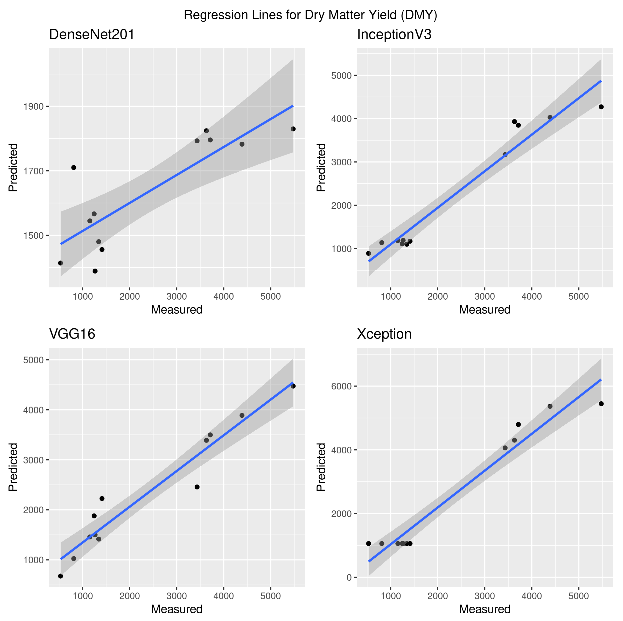
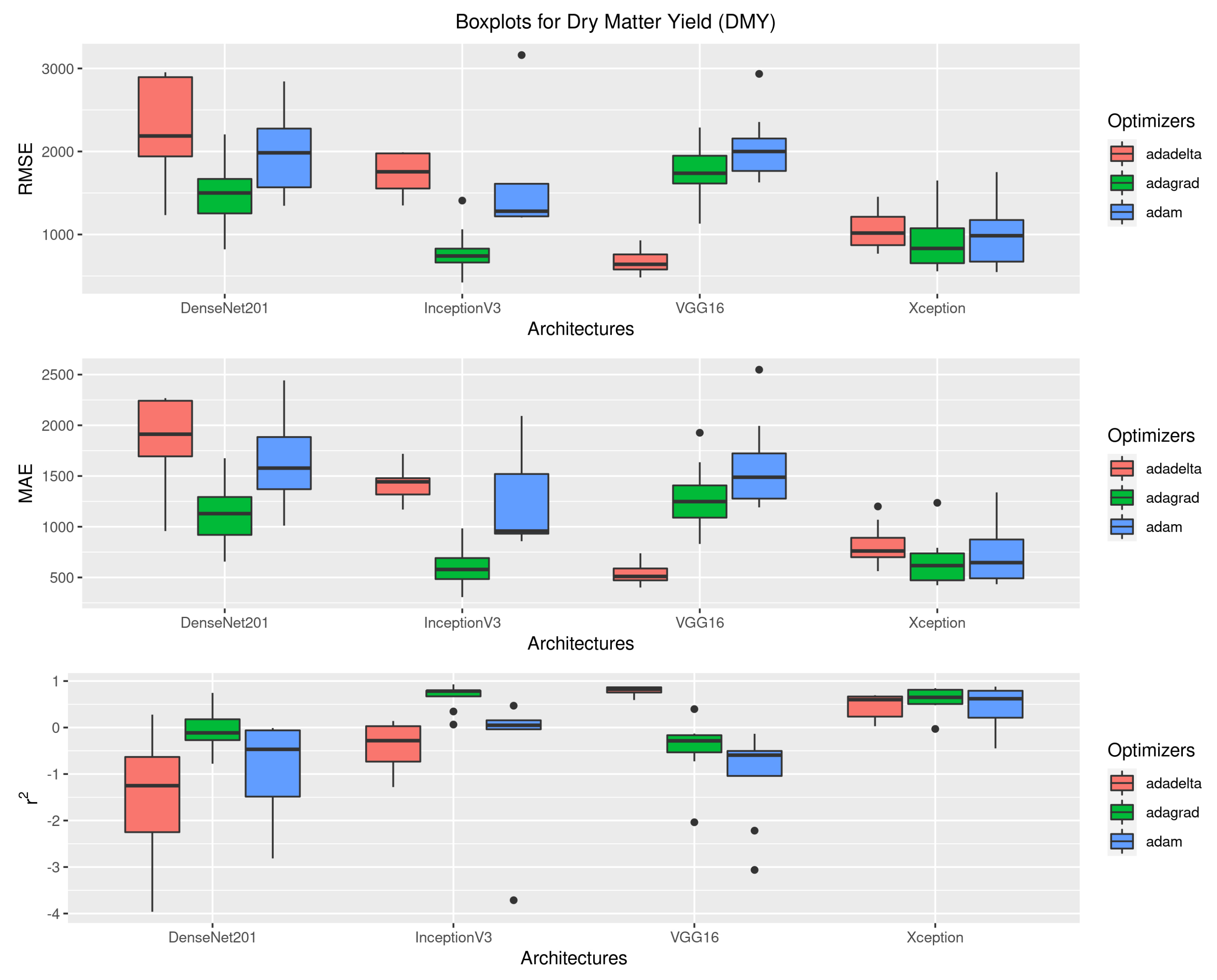
3.1. Dry Matter Yield

The boxplots in Figure 3 show the RMSE, MAE and $r^2$ results for all configurations of architectures and optimizers. It can be seen that the configuration choice had a great impact on the overall performance metrics, where VGG16 with Adadelta optimizer obtained the best values for all metrics and fewer outliers. The median values for the best RMSE, MAE, nMAE and $r^2$ results (VGG16+Adadelta) were, respectively, 640.96 kg DM/ha, 509.87 kg DM/ha, 19.22% and 0.82. The best values, among all eight runs, were 482.12 kg DM/ha, 400.53 kg DM/ha and 0.88, for RMSE, MAE and $r^2$, respectively. DenseNet201 obtained the worst accuracy, with all $r^2$ values being negative. Xception was least affected by the optimization strategy, with a good balance of the performance metrics. The performance of VGG16 was lower when the algorithm was coupled with the Adagrad or Adam optimizers. The InceptionV3-based network had some extremely large outliers for the Adam optimizer, which were removed from the graph.

Figure 4 presents the predicted versus measured DMY values for the best run of the 8-fold cross-validation of each architecture configuration. The Xception boxplot results were overly optimistic, as, for the smaller DMY values, the model simply predicted the same outputs.

Table 4. Dry matter yield root mean squared error (RMSE) (kg DM/ha), mean absolute error (MAE) (kg DM/ha), normalized mean absolute error (nMAE) (%) and coefficient of determination ($r^2$) means and standard values over the 8-fold test set for all the architectures and optimizers.

Architecture	Optimizer	RMSE (kg DM/ha)	MAE (kg DM/ha)	nMAE (%)	${\mathit{r}}^2$
DenseNet201	Adadelta	2278.95 (608.69)	1858.41 (442.83)	70.06	−1.49 (1.32)
DenseNet201	Adagrad	1494.85 (414.68)	1141.18 (334.93)	43.02	−0.06 (0.48)
DenseNet201	Adam	1984.89 (508.92)	1634.87 (443.55)	61.63	−0.89 (1.04)
InceptionV3	Adadelta	1739.52 (242.13)	1413.80 (172.38)	53.30	−0.43 (0.57)
InceptionV3	Adagrad	801.72 (303.11)	606.96 (212.71)	22.88	0.66 (0.29)
InceptionV3	Adam	8830.16 (10,405.33)	3615.15 (3486.56)	136.29	−72.43 (115.08)
VGG16	Adadelta	668.79 (144.07)	538.07 (111.12)	20.28	0.79 (0.10)
VGG16	Adagrad	1759.99 (368.30)	1293.27 (348.31)	48.75	−0.46 (0.71)
VGG16	Adam	2064.42 (420.08)	1610.65 (460.89)	60.72	−1.03 (1.03)
Xception	Adadelta	1066.17 (264.53)	819.55 (213.82)	30.90	0.46 (0.26)
Xception	Adagrad	915.36 (366.36)	667.72 (265.45)	25.17	0.59 (0.29)
Xception	Adam	997.50 (411.66)	724.23 (307.57)	27.30	0.45 (0.47)

shows the mean values for all the performance metrics. InceptionV3+Adam presented extremely high standard deviations for the Adam optimizer. VGG16 achieved the best mean values for all metrics, which were slightly lower than the median values, but not as much as with some other configurations, where a huge gap could be seen due to outliers. InceptionV3+Adagrad obtained the second best $r^2$ value, emphasizing the importance of testing different optimizers for different architectures when dealing with regression problems and small datasets.

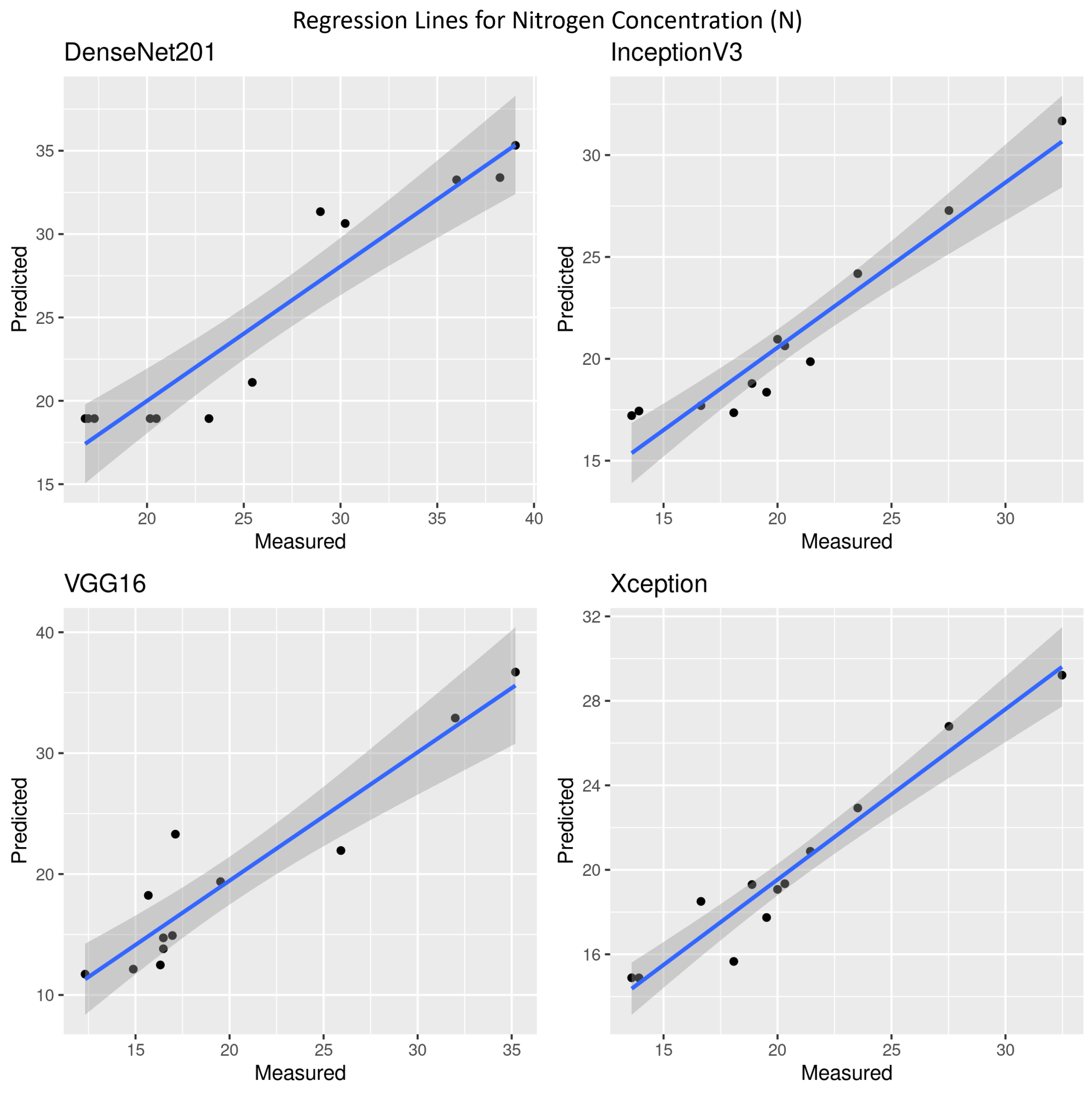
3.2. Nitrogen Concentration

The experiments to estimate the nitrogen concentration resulted in the boxplots presented in Figure 5. As with DMY, VGG16+Adadelta had the highest median $r^2$ and the most stable results. This configuration yielded RMSE = 2.56 g N/kg DM and MAE = 2.27 g N/kg DM (10.39%) as minimum values and the maximum $r^2$ = 0.82. The respective median values were RMSE = 3.90 g N/kg DM, MAE = 3.16 g N/kg DM and $r^2$ = 0.74. For DenseNet201, InceptionV3 and Xception, the best results were achieved using Adagrad.

The regression lines for nitrogen concentration estimation, using the best results for each architecture, are shown in Figure 6. Means and standard deviations are shown in

Table 5. Nitrogen concentration root mean squared error (RMSE), mean absolute error (MAE), normalized MAE (nMAE) and coefficient of determination ($r^2$) means and standard values over the 8-fold test set for all the architectures and optimizers.

Architecture	Optimizer	RMSE (g N/kg DM)	MAE (g N/kg DM)	nMAE (%)	${\mathit{r}}^2$
DenseNet201	Adadelta	14.66 (2.11)	11.68 (1.75)	52.94	−3.49 (1.87)
DenseNet201	Adagrad	7.23 (2.45)	5.76 (2.10)	26.11	−0.07 (0.43)
DenseNet201	Adam	8.02 (1.70)	6.27 (1.59)	28.42	−0.17 (0.24)
InceptionV3	Adadelta	10.28 (2.53)	8.32 (2.25)	37.71	−1.21 (1.24)
InceptionV3	Adagrad	3.87 (1.59)	3.11 (1.31)	14.10	0.70 (0.20)
InceptionV3	Adam	12.23 (7.59)	7.74 (3.57)	35.08	−3.06 (5.43)
VGG16	Adadelta	3.72 (0.66)	3.11 (0.53)	14.10	0.73 (0.07)
VGG16	Adagrad	8.11 (2.60)	6.45 (2.44)	29.24	−0.29 (0.67)
VGG16	Adam	7.45 (1.32)	5.99 (1.41)	27.15	−0.07 (0.10)
Xception	Adadelta	6.91 (1.58)	5.30 (1.17)	24.02	−0.01 (0.53)
Xception	Adagrad	3.80 (1.30)	2.96 (0.94)	13.42	0.71 (0.14)
Xception	Adam	8.65 (8.01)	5.94 (3.80)	26.92	−1.27 (4.36)

. Despite VGG16 having the highest $r^2$ mean value, Xception achieved the lowest mean RMSE and MAE.

4. Discussion

This study focused on a deep learning-based approach to estimate the biomass (DMY) and nitrogen concentration of grass sward for silage from RGB orthomosaics at four harvest dates of primary growth. We compared the performance of four CNN architectures (DenseNet201, InceptionV3, VGG16 and Xception) with three different optimizers. The best average results of the cross-validation were clearly achieved by the VGG16 architecture with Adadelta optmizer, RMSE of 668.79 kg DM/ha and $r^2$ of 0.79, for DMY. While, for nitrogen concentration, VGG16+Adadelta (RMSE 3.72 g N/kg DM and $r^2$ 0.73), Xception+Adagrad (RMSE 3.80 g N/kg DM and $r^2$ 0.71) and InceptionV3+Adagrad (RMSE 3.87 g N/kg DM and $r^2$ 0.70) yielded similar average accuracy metrics. Overall, DenseNet201 presented the worst results for both DMY and N. Nevavuori et al. [13] also obtained the best results for their CNN architecture using the Adadelta optimizer for predicting wheat and barley yield. An architecture based on VGGNet also presented good results to predict the aboveground biomass of winter wheat [12].

Several configurations resulted in negative $r^2$, indicating that they could not learn much using this dataset. DenseNet201, for instance, presented all $r^2$ median values below zero. It is interesting to note that the now classic VGG16, which is usually surpassed by the other three newer architectures for classification problems, presented the best results in this regression problem, reinforcing the importance of more studies related to deep regression in the remote sensing scenario. In previous study by Viljanen et al. [29] using the same RGB image data and a multilinear regression approach, the DMY RMSE was 1190 kg DM/ha, and using a non-linear approach, random forest, the RMSE was 1000 kg DM/ha, clearly worse than the results with VGG16+Adadelta presented in this study. The authors improved the random forest RMSE for DMY by combining RGB image data with 3D features extracted from photogrammetric crop height models (CHM) (RMSE 430 kg DM/ha), which was expected since the best CHM feature was reported to be strongly correlated (0.85–0.97) with the DMY during the four measurement dates. Further improvements to RMSE were still achieved by Viljanen et al. [29] when combining the RGB and NIR bands to compute multispectral vegetation indices (RMSE 420 kg DM/ha). For the same area and reference data, Oliveira et al. [8] reported an RMSE of 389 kg DM/ha, for DMY, but using 36 hyperspectral bands, vegetation indices and 3D features.

Other works using CNN-based approaches for grass biomass are still rare. de Oliveira et al. [19] investigated the dry matter yield estimation using CNN regression and achieved an RSME of 413–507 kg DM/ha for total dry matter yield with different models. Castro et al. [18] proposed a similar CNN-based approach for green biomass estimation in a pasture site in Brazil and reported a mean absolute error of 13%. However, the direct comparison of different studies is not straightforward because many aspects, such as the presence of different plants, variability of reference field measurements and validation methods, can affect the results.

In the study of Oliveira et al. [8], the same RGB image data combined with 3D features were used to estimate nitrogen concentration using a conventional machine learning method, random forest, and the RMSE was 2.85 g N/kg DM (normalized RMSE 12.90%), which is slightly better than the CNN (VGG16+Adadelta). However, it should be noted that the CNN was not fed with 3D features and 20% of samples were used for validation, while, with random forest, the leave-one-out cross-validation was applied, which might have slightly impacted the values. As with DMY, the estimation accuracy of the nitrogen concentration using random forest was further improved when the hyperspectral features were added to the model [8]. Higher spectral resolution has been reported to improve the accuracy of nitrogen estimation using conventional machine learning methods also by Askari et al. [25], Togeiro de Alckmin et al. [37] and Barnetson et al. [27]. However, hyperspectral sensors are not only more expensive than RGB cameras but also require more complex preprocessing steps.

Other studies where UAV-based RGB image data and CNN methods have been used to estimate biomass and nitrogen concentration in grasslands are still rare. Instead, CNN has been employed for this task with data from hand-held field spectroscopy [38]. These authors achieved an RMSE of 14% ($r^2$ = 0.72) using 1D-CNN in the study area in New Zealand. Furthermore, Michez et al. [26] proposed conventional multilinear regression models for grass crude protein, which is nearly linked to nitrogen content, using low-cost UAV-based data, and reported the RMSE of 0.93% and $r^2$ of 0.54 at best.

The proposed approach can be described as a data-driven, non-parametric, nonlinear regression method in comparison to physical-based models, based on radiative transfer models. Specifically, for nitrogen estimation, hybrid methods utilizing machine learning and radiative transfer models have yielded promising results, such as a study by Berger et al. [39] using satellite data, where they achieved an RMSE of 2.1 g/m${}^2$.

As our approach is UAV-based, it is applicable locally with high spatial resolution and also during overcast weather, in contrast to optical satellite-based approaches. Furthermore, the use of only RGB image data can be considered an interesting and feasible strategy for practical applications since this sensor is low-cost and less computationally expensive in comparison to approaches using 3D or hyperspectral data. However, additional studies using different types of sensors will contribute even further to the development of CNN approaches for grassland applications.

In the Nordic countries, the grass is harvested 2–4 times in the summer season. This study investigated only the primary growth, where the speed of growth is higher compared to regrowths of the grass and, thus, they may need to have their own models [8]. Our study was also conducted in a single field; thus, the transferability of the models to other fields, grass types and biomes should be further investigated.

5. Conclusions

This study investigated different CNN architectures and optimizers to estimate the biomass (DMY) and nitrogen concentration of grass swards for silage from RGB orthomosaics produced from images captured by a UAV. The best estimation accuracy metrics were achieved using the VGG16 architecture with the Adadelta optimizer for both DMY and nitrogen concentration. Xception with the Adagrat optimizer obtained similar performance as VGG16 for nitrogen concentration. The feasibility of CNNs and RGB UAV data for grass biomass and nitrogen estimation has rarely been examined in the literature. Overall, our findings are consistent with other studies in the literature, showing that the proposed approach can be considered a potential technique for grass management tasks, such as planning additional fertilization and estimating the optimal time for harvesting the crop, using low-cost RGB data. Although the results from cross-validation were promising, further experiments using, for instance, larger datasets, different test sites and different types of sensors will be of great importance to explore the potential of the CNN approaches, as well as to increase the generalizability of the models.

References

1. Rockström, J.; Williams, J.; Daily, G.; Noble, A.; Matthews, N.; Gordon, L.; Wetterstrand, H.; DeClerck, F.; Shah, M.; Steduto, P.; et al. Sustainable intensification of agriculture for human prosperity and global sustainability. Ambio 2017, 46, 4–17. [Google Scholar] [CrossRef] [PubMed] [Green Version]
2. O’Mara, F.P. The role of grasslands in food security and climate change. Ann. Bot. 2012, 110, 1263–1270. [Google Scholar] [CrossRef] [PubMed] [Green Version]
3. Bengtsson, J.; Bullock, J.; Egoh, B.; Everson, C.; Everson, T.; O’Connor, T.; O’Farrell, P.; Smith, H.; Lindborg, R. Grasslands—More important for ecosystem services than you might think. Ecosphere 2019, 10, e02582. [Google Scholar] [CrossRef]
4. Korhonen, P.; Palosuo, T.; Persson, T.; Höglind, M.; Jégo, G.; Van Oijen, M.; Gustavsson, A.M.; Bélanger, G.; Virkajärvi, P. Modelling grass yields in northern climates–a comparison of three growth models for timothy. Field Crops Res. 2018, 224, 37–47. [Google Scholar] [CrossRef]
5. Reinermann, S.; Asam, S.; Kuenzer, C. Remote sensing of grassland production and management—A review. Remote Sens. 2020, 12, 1949. [Google Scholar] [CrossRef]
6. Pajares, G. Overview and current status of remote sensing applications based on unmanned aerial vehicles (UAVs). Photogramm. Eng. Remote Sens. 2015, 81, 281–330. [Google Scholar] [CrossRef] [Green Version]
7. Manfreda, S.; McCabe, M.F.; Miller, P.E.; Lucas, R.; Pajuelo Madrigal, V.; Mallinis, G.; Ben Dor, E.; Helman, D.; Estes, L.; Ciraolo, G.; et al. On the use of unmanned aerial systems for environmental monitoring. Remote Sens. 2018, 10, 641. [Google Scholar] [CrossRef] [Green Version]
8. Oliveira, R.A.; Näsi, R.; Niemeläinen, O.; Nyholm, L.; Alhonoja, K.; Kaivosoja, J.; Jauhiainen, L.; Viljanen, N.; Nezami, S.; Markelin, L.; et al. Machine learning estimators for the quantity and quality of grass swards used for silage production using drone-based imaging spectrometry and photogrammetry. Remote Sens. Environ. 2020, 246, 111830. [Google Scholar] [CrossRef]
9. Kamilaris, A.; Prenafeta-Boldú, F.X. Deep learning in agriculture: A survey. Comput. Electron. Agric. 2018, 147, 70–90. [Google Scholar] [CrossRef] [Green Version]
10. Osco, L.P.; Junior, J.M.; Ramos, A.P.M.; de Castro Jorge, L.A.; Fatholahi, S.N.; de Andrade Silva, J.; Matsubara, E.T.; Pistori, H.; Gonçalves, W.N.; Li, J. A review on deep learning in UAV remote sensing. Int. J. Appl. Earth Obs. Geoinf. 2021, 102, 102456. [Google Scholar] [CrossRef]
11. Kattenborn, T.; Leitloff, J.; Schiefer, F.; Hinz, S. Review on Convolutional Neural Networks (CNN) in vegetation remote sensing. ISPRS J. Photogramm. Remote Sens. 2021, 173, 24–49. [Google Scholar] [CrossRef]
12. Ma, J.; Li, Y.; Chen, Y.; Du, K.; Zheng, F.; Zhang, L.; Sun, Z. Estimating above ground biomass of winter wheat at early growth stages using digital images and deep convolutional neural network. Eur. J. Agron. 2019, 103, 117–129. [Google Scholar] [CrossRef]
13. Nevavuori, P.; Narra, N.; Lipping, T. Crop yield prediction with deep convolutional neural networks. Comput. Electron. Agric. 2019, 163, 104859. [Google Scholar] [CrossRef]
14. Yang, Q.; Shi, L.; Han, J.; Zha, Y.; Zhu, P. Deep convolutional neural networks for rice grain yield estimation at the ripening stage using UAV-based remotely sensed images. Field Crops Res. 2019, 235, 142–153. [Google Scholar] [CrossRef]
15. Yang, W.; Nigon, T.; Hao, Z.; Paiao, G.D.; Fernández, F.G.; Mulla, D.; Yang, C. Estimation of corn yield based on hyperspectral imagery and convolutional neural network. Comput. Electron. Agric. 2021, 184, 106092. [Google Scholar] [CrossRef]
16. Chen, Y.; Lee, W.S.; Gan, H.; Peres, N.; Fraisse, C.; Zhang, Y.; He, Y. Strawberry yield prediction based on a deep neural network using high-resolution aerial orthoimages. Remote Sens. 2019, 11, 1584. [Google Scholar] [CrossRef] [Green Version]
17. Apolo-Apolo, O.; Martínez-Guanter, J.; Egea, G.; Raja, P.; Pérez-Ruiz, M. Deep learning techniques for estimation of the yield and size of citrus fruits using a UAV. Eur. J. Agron. 2020, 115, 126030. [Google Scholar] [CrossRef]
18. Castro, W.; Marcato Junior, J.; Polidoro, C.; Osco, L.; Gonçalves, W.; Rodrigues, L.; Santos, M.; Jank, L.; Barrios, S.; Valle, C.; et al. Deep Learning Applied to Phenotyping of Biomass in Forages with UAV-Based RGB Imagery. Sensors 2020, 20, 4802. [Google Scholar] [CrossRef]
19. de Oliveira, G.S.; Marcato Junior, J.; Polidoro, C.; Osco, L.P.; Siqueira, H.; Rodrigues, L.; Jank, L.; Barrios, S.; Valle, C.; Simeão, R.; et al. Convolutional Neural Networks to Estimate Dry Matter Yield in a Guineagrass Breeding Program Using UAV Remote Sensing. Sensors 2021, 21, 3971. [Google Scholar] [CrossRef]
20. Berger, K.; Verrelst, J.; Feret, J.B.; Wang, Z.; Wocher, M.; Strathmann, M.; Danner, M.; Mauser, W.; Hank, T. Crop nitrogen monitoring: Recent progress and principal developments in the context of imaging spectroscopy missions. Remote Sens. Environ. 2020, 242, 111758. [Google Scholar] [CrossRef]
21. Geipel, J.; Link, J.; Wirwahn, J.A.; Claupein, W. A programmable aerial multispectral camera system for in-season crop biomass and nitrogen content estimation. Agriculture 2016, 6, 4. [Google Scholar] [CrossRef] [Green Version]
22. Liu, Y.; Cheng, T.; Zhu, Y.; Tian, Y.; Cao, W.; Yao, X.; Wang, N. Comparative analysis of vegetation indices, non-parametric and physical retrieval methods for monitoring nitrogen in wheat using UAV-based multispectral imagery. In Proceedings of the 2016 IEEE International Geoscience and Remote Sensing Symposium (IGARSS), Beijing, China, 10–15 July 2016; pp. 7362–7365. [Google Scholar]
23. Näsi, R.; Honkavaara, E.; Blomqvist, M.; Lyytikäinen-Saarenmaa, P.; Hakala, T.; Viljanen, N.; Kantola, T.; Holopainen, M. Remote sensing of bark beetle damage in urban forests at individual tree level using a novel hyperspectral camera from UAV and aircraft. Urban For. Urban Green. 2018, 30, 72–83. [Google Scholar] [CrossRef]
24. Capolupo, A.; Kooistra, L.; Berendonk, C.; Boccia, L.; Suomalainen, J. Estimating plant traits of grasslands from UAV-acquired hyperspectral images: A comparison of statistical approaches. ISPRS Int. J. Geo-Inf. 2015, 4, 2792–2820. [Google Scholar] [CrossRef]
25. Askari, M.S.; McCarthy, T.; Magee, A.; Murphy, D.J. Evaluation of grass quality under different soil management scenarios using remote sensing techniques. Remote Sens. 2019, 11, 1835. [Google Scholar] [CrossRef] [Green Version]
26. Michez, A.; Philippe, L.; David, K.; Sébastien, C.; Christian, D.; Bindelle, J. Can low-cost unmanned aerial systems describe the forage quality heterogeneity? Insight from a Timothy Pasture case study in Southern Belgium. Remote Sens. 2020, 12, 1650. [Google Scholar] [CrossRef]
27. Barnetson, J.; Phinn, S.; Scarth, P. Estimating plant pasture biomass and quality from UAV imaging across Queensland’s Rangelands. AgriEngineering 2020, 2, 523–543. [Google Scholar] [CrossRef]
28. Peel, M.C.; Finlayson, B.L.; McMahon, T.A. Updated world map of the Köppen-Geiger climate classification. Hydrol. Earth Syst. Sci. 2007, 11, 1633–1644. [Google Scholar] [CrossRef] [Green Version]
29. Viljanen, N.; Honkavaara, E.; Näsi, R.; Hakala, T.; Niemeläinen, O.; Kaivosoja, J. A novel machine learning method for estimating biomass of grass swards using a photogrammetric canopy height model, images and vegetation indices captured by a drone. Agriculture 2018, 8, 70. [Google Scholar] [CrossRef] [Green Version]
30. Huang, G.; Liu, Z.; Weinberger, K.Q. Densely Connected Convolutional Networks. In Proceedings of the IEEE Conference on Computer Vision and Pattern Recognition (CVPR), Honolulu, HI, USA, 21–26 July 2017. [Google Scholar]
31. Szegedy, C.; Vanhoucke, V.; Ioffe, S.; Shlens, J.; Wojna, Z. Rethinking the Inception Architecture for Computer Vision. In Proceedings of the IEEE Conference on Computer Vision and Pattern Recognition, Las Vegas, NV, USA, 27–30 June 2016. [Google Scholar]
32. Simonyan, K.; Zisserman, A. Very Deep Convolutional Networks for Large-Scale Image Recognition. arXiv 2014, arXiv:1409.1556. [Google Scholar]
33. Chollet, F. Xception: Deep Learning with Depthwise Separable Convolutions. arXiv 2016, arXiv:1610.02357. [Google Scholar]
34. Zeiler, M.D. ADADELTA: An Adaptive Learning Rate Method. arXiv 2012, arXiv:1212.5701. [Google Scholar]
35. Duchi, J.; Hazan, E.; Singer, Y. Adaptive subgradient methods for online learning and stochastic optimization. J. Mach. Learn. Res. 2011, 12, 2121–2159. [Google Scholar]
36. Kingma, D.P.; Ba, J. Adam: A Method for Stochastic Optimization, 2014. arXiv 2014, arXiv:1412.6980. [Google Scholar]
37. Togeiro de Alckmin, G.; Lucieer, A.; Roerink, G.; Rawnsley, R.; Hoving, I.; Kooistra, L. Retrieval of crude protein in perennial ryegrass using spectral data at the Canopy level. Remote Sens. 2020, 12, 2958. [Google Scholar] [CrossRef]
38. Pullanagari, R.; Dehghan-Shoar, M.; Yule, I.J.; Bhatia, N. Field spectroscopy of canopy nitrogen concentration in temperate grasslands using a convolutional neural network. Remote Sens. Environ. 2021, 257, 112353. [Google Scholar] [CrossRef]
39. Berger, K.; Verrelst, J.; Féret, J.B.; Hank, T.; Wocher, M.; Mauser, W.; Camps-Valls, G. Retrieval of aboveground crop nitrogen content with a hybrid machine learning method. Int. J. Appl. Earth Obs. Geoinf. 2020, 92, 102174. [Google Scholar] [CrossRef]
Figure 1. Workflow of the main steps performed in this study.
Agronomy 12 01352 g001
Figure 2. Location of the study area in Jokioinen, Finland. Orthomosaic for 15 June, as well as the location of the harvesting for the reference sample plots and their nitrogen fertilizer rates, from 0 to 150 kg/ha, indicated inside the polygons. On the right side, from top to bottom, examples of image patches extracted from the orthomosaics.
Agronomy 12 01352 g002
Figure 3. Dry matter yield root mean squared error (RMSE) [kg DM/ha], mean absolute error (MAE) [kg DM/ha] and coefficient of determination ( r 2 ) boxplots for all 4 architectures (DenseNet201, InceptionV3, VGG16 and Xception) and the 3 optimizers (Adadelta, Adagrad and Adam) used. The data came from the 8 runs (i.e., 8 cross-validation folds) of each configuration (architecture+optimizer) over the DMY test set. To improve the readability, 3 extreme outliers (RMSE > 10.000 kg DM/ha) for InceptionV3 optimized by Adam have been removed.
Agronomy 12 01352 g003
Figure 4. XY graphics for predicted versus measured dry matter yield (DMY) (kg DM/ha) points arising from the best run for each architecture. The regression lines are shown in blue and the grey area is the confidence interval.
Agronomy 12 01352 g004
Figure 5. Nitrogen concentration root mean squared error (RMSE) (g N/kg DM), mean absolute error (MAE) (g N/kg DM) and coefficient of determination ( r 2 ) boxplots for all four architectures (DenseNet201, InceptionV3, VGG16 and Xception) and the three optimizers (Adadelta, Adagrad and Adam) used. The data came from the 8 runs (i.e., 8 cross-validation folds) of each configuration (architecture+optimizer) over the N test set.
Agronomy 12 01352 g005
Figure 6. XY graphics for predicted versus measured nitrogen concentration (N) points arising from the best run for each architecture. The regression lines are shown in blue and the grey area is the confidence interval.
Agronomy 12 01352 g006