A Simplified Approach to the Evaluation of the Influences of Key Factors on Agricultural Tractor Fuel Consumption during Heavy Drawbar Tasks under Field Conditions

Abstract

The optimization of energy input on agricultural farms, such as through improved fuel consumption, is currently under investigation in agricultural mechanization research with the aim of achieving economic and environmental goals. In previous research, we developed a simplified algorithm focused on defining the most efficient tractor–implement combination considering the factors that most influence this aspect. The ASABE (American Society of Agricultural and Biological Engineers) equation for calculating the drawbar pull force was adopted to fit the results to the soil conditions. Agricultural tires of different sizes were tested at different pressure settings under field conditions to assess differences in drawbar force. The resulting algorithm underwent a linear regression analysis to achieve a simplified equation for assessing the optimal wheel-slip, mass, engine power, and tire pull force properties during drawbar works that result in optimal fuel consumption with a minimal tractor efficiency impairment. Using a specific probability density function, the Monte Carlo Simulation method introduced randomness into the input and runs a sufficiently large number of trials to identify the most probable output. The result is a simplified algorithm that can be used to investigate the effects of certain parameters on fuel consumption; however, it can be adapted to evaluate the effects of different implements, tires, engine settings, or fleet management methods on fuel consumption.

1. Introduction

The optimization of energy inputs for agricultural activities is becoming increasingly important, even more so when considering nonrenewable energy sources and emission mitigation. As far as tractors are concerned, from an energy perspective, heavy drawbar work (e.g., plowing) is one of the most critical tasks because of the engine power requirement and the number of factors affecting the tractive efficiency of the machine. Standard measurement methods [1] make it possible to obtain comparable data and develop algorithms on tractor dynamics and efficiency; however, such standards recommend that the machine is run on either asphalt or concrete test tracks that do not represent standard agricultural working conditions.

Many studies on tractor efficiency have focused on power efficiency by varying the engine, driveline, and tires [2,3,4,5]. However, traction performance optimization, not only in terms of material engineering but, above all, concerning labor and energy efficiency, remains of primary importance [6,7,8,9,10,11,12], particularly in light of investigations that have delved deeper into the effects of soil properties on tractive efficiency and performance [13,14].

Cutini et al. [15] investigated the fuel consumption of 100 tractors of different weights and engine power levels according to the OECD Code 2 standard test and achieved a regression equation that served as the starting point to analyze the driveline efficiency and the power lost through both rolling resistance and slippage. The extension of such an equation to soil conditions foresaw the application of a horizontal force to the agricultural tractor drawbar while running it on a field [16,17]. The measurement of the primary tractor performance outputs in the field (i.e., drawbar force, forward speed, wheel-slip) was performed with four tractors with different sets of tires over a total of 84 tests, and the results highlighted the relationship of the drawbar force with wheel slippage [18,19].

In this work, the Monte Carlo Simulation (MCS) method was used to explore the effect that tractor engine adjustments (i.e., load and speed [20]), tractor mass, wheel-slip, and the tire traction properties have on tractor-specific fuel consumption. The impacts of each of these variables were also evaluated. The output of the MCS highlighted the most influential variables, and the results were verified afterwards with specific experimental activity.

This paper is structured as follows:

• Section 2 reports the reference equations that were chosen, the variables they contain, the way the MCS algorithm was developed, and the experimental trials carried out for the validation activity.
• Section 3 shows the MCS output, how it relates to the random input variables, and their importance, as determined by the linear regression analysis. Section 3.2 and Section 3.3 show the results of the experimental trials and the validation process entered when compared with the MCS output.
• Section 4 and Section 5 discuss the achieved results and present the conclusions of the study.

2. Materials and Methods

2.1. The Reference Equations

A summary of the algorithms used in the present work and presented in the cited literature is as follows:

The equations used to set up the methodology belong to different standards. Tractors use internal combustion engines to power farm machines. However, power losses occur when exerting power through the drive wheels, the PTO shaft, and the hydraulic system. When performing heavy drawbar tasks (e.g., plowing), the first step is the calculation of the drawbar power, that is, the power that the machine makes available to users. For this, it is necessary to assess the Specific Fuel Consumption per hectare (SFC_ha). The power at the drawbar (P_db) results from the measurement of the applied horizontal force and the forward velocity, as shown by Equation (1) [21]:

$$P_{db}=F·\overrightarrow{v}$$

(1)

where the power at the drawbar (P_db, kW) is the product of the drawbar pull (F) and the vehicle velocity ($\overrightarrow{v}$) in the direction of travel. The drawbar pull is the force in the direction of travel that the vehicle produces at the drawbar or hitch.

However, to calculate the specific fuel consumption (SFC) of the power at the drawbar, the power at the engine that results from Equation (2) needs to be considered. Here, the calculation of the maximum power available at the drawbar considers the losses in the maximum power of the engine [15,22]. Hereinafter, the power of the engine is always referred to as the PTO, in compliance with the OECD Code 2 [1].

$$P_{db}=\alpha ·P_{PTO}-P_{vd}-P_s$$

(2)

where

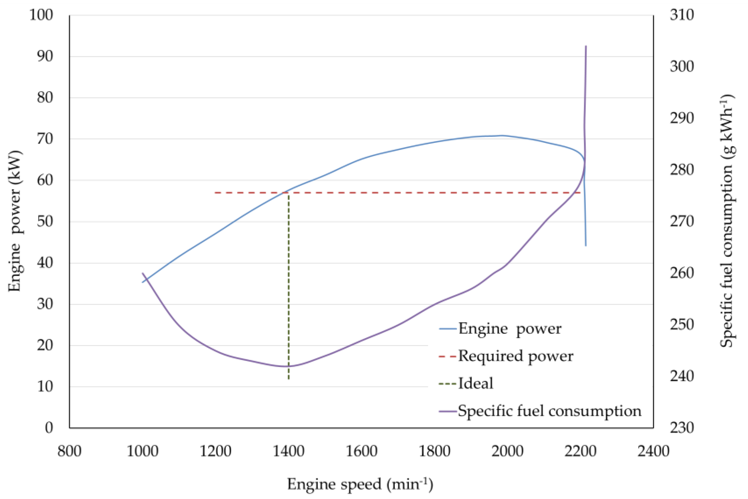
• P_db is the power at the drawbar (kW);
• P_PTO is the maximum engine power measured at power take-off [1] (kW);
• P_vd is the power used for the vehicle’s displacement (kW);
• P_s is the power lost due to slippage (kW);
• α is the driveline efficiency coefficient (dimensionless).

Inserting the coefficients from the linear regression analysis presented in the study by Cutini et al. [19] into Equation (2) results in Equations (3) and (4):

$$P_{db}=0.92·P_{PTO}-0.07·M·\overrightarrow{v}-0.009·P_{PTO}·s$$

(3)

$$P_{PTO}=(P_{db}+0.07·M·\overrightarrow{v})·{\left(0.92-0.009·s\right)}^{-1}$$

(4)

where the power at the drawbar relates to the following:

• P_PTO is the maximum power of the engine measured at power take-off [1] (kW)
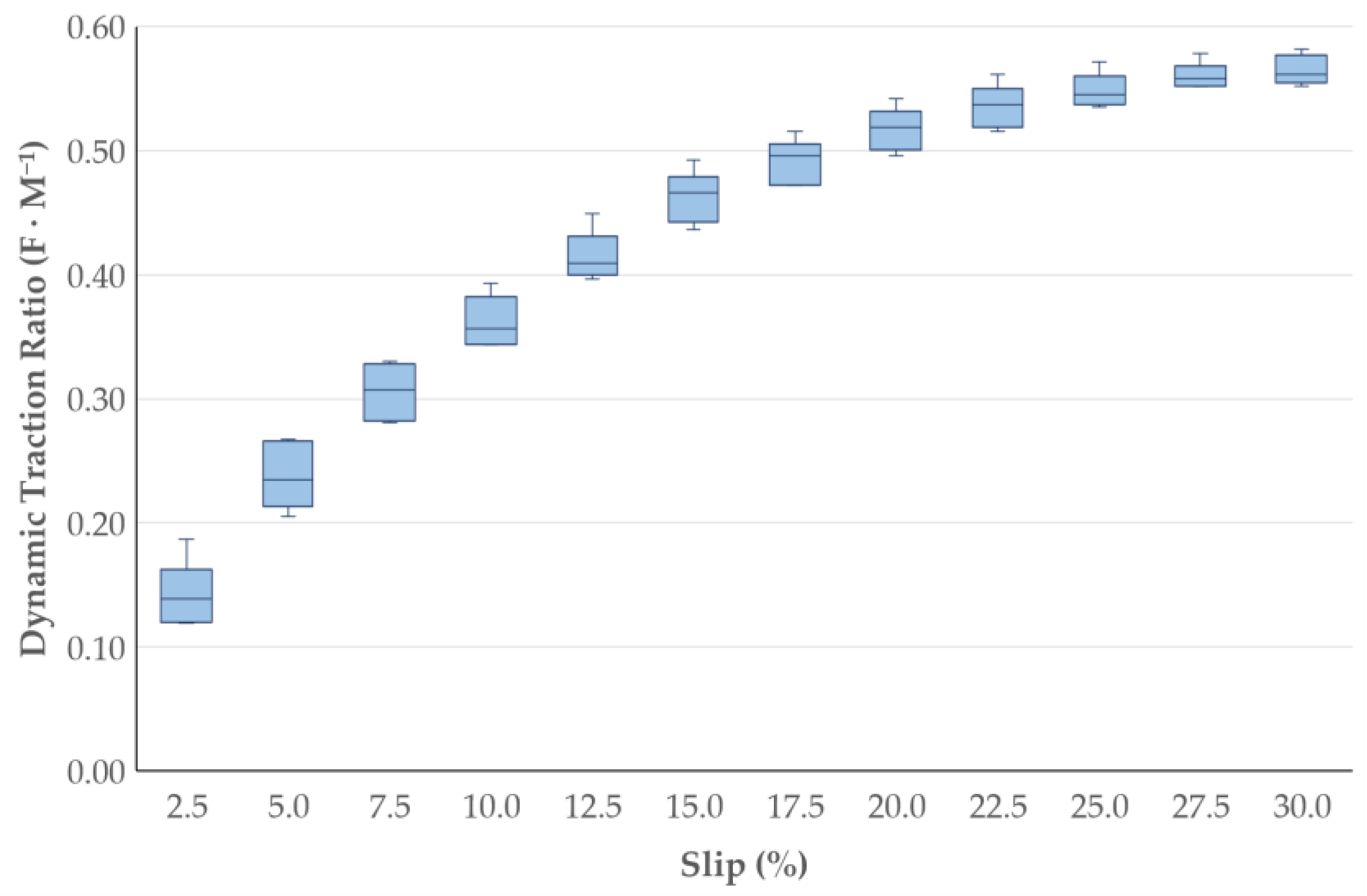
• M is the dynamic wheel load, in force units, normal to the soil surface ($\stackrel{\rightharpoonup }{kN}$);
• $\overrightarrow{v}$ is the forward velocity (m s⁻¹);
• s is the wheel slip (dimensionless).

The constants with values of 0.92 and 0.07 are the driveline efficiency coefficient (α in Equation (2)) and the motion resistance ratio coefficient on terrain soil, which affects the P_vd. They both comply with ASAE standard recommendations [18].

The target of this study is the tractor-specific fuel consumption per hectare of tilled soil (SFC_ha, kg_fuel ha⁻¹) that results from Equation (5):

$$SF{C}_{ha}=h_{ha}·SF{C}_{kW}·P_{PTO}·{10}^{-3}$$

(5)

where

• h_ha are the worked hours required for 1 hectare (hours ha⁻¹, from Equation (5));
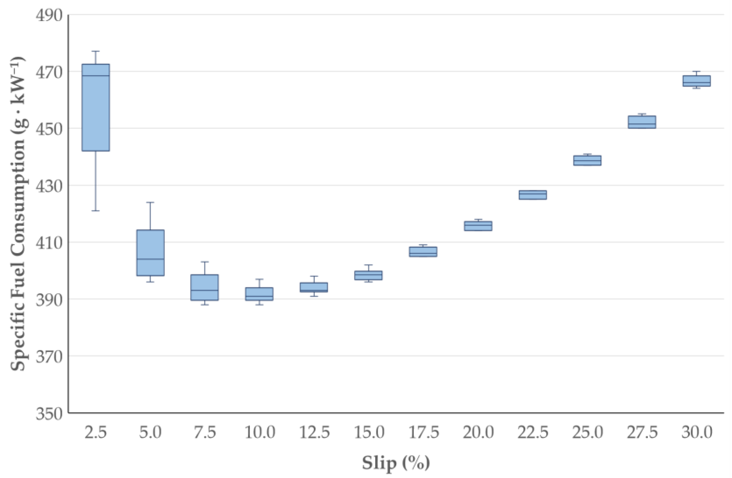
• SFC_kW is the specific fuel consumption of the engine (g_fuel kWh⁻¹);
• P_PTO is the power provided by the vehicle’s engine (kW).

The h_ha calculation (Equation (6)) results from measurements of the operating conditions when the operator runs the tractor at a constant speed without turning the steering wheel:

$$h_{ha}=W^{-1}·{(3600·\overrightarrow{v})}^{-1}·{10}^4$$

(6)

where

• W is the working width of the implement (m);
• $\overrightarrow{v}$ is the forward velocity (m s⁻¹).

The second step focuses on the influence that tire traction properties have on the SFC_ha. There is a need to introduce a new variable (Grip, dimensionless) to justify the variations in the dynamic traction ratio under operating conditions.

By defining F and assigning s, the ASAE 2003 standard [21] allows the dynamic wheel load to be calculated. Therefore, it is possible to calculate the dynamic traction ratio (T_r; dimensionless [21]), which is the ratio of drawbar pull (F) to the dynamic load on the vehicle (Equation (7)).

$$T_r=F·M^{-1}$$

(7)

The dynamic traction ratio alone does not account for the tractive properties of the tires. Therefore, a new index (called specific dynamic traction ratio-$T_r^{\prime }$-Equation (8)) that includes the features of the tires results from its multiplication with the grip coefficient (Grip, dimensionless) and ranges from 0.85 to 1.15 (Section 2.2).

$$T_r^{\prime }=F·M^{-1}·Grip$$

(8)

Of course, such a change affects the calculation of M and, consequently, the parameters in Equation (4), which vary as follows (Equation (9)):

$$P_{PTO}=\left(F·\overrightarrow{v}+0.07·F·T_r{}^{-1}·Grip·\overrightarrow{v}\right)·{\left(\mathsf{\alpha }-0.009·s\right)}^{-1}$$

(9)

Finally, by substituting the value of P_PTO into Equation (4), the algorithm used for the Monte Carlo analysis changes into Equation (10) (CREA-IT equation):

$$SF{C}_{ha}=h_{ha}·SF{C}_{kW}·\left(F·\overrightarrow{v}+0.07·F·T_r{}^{-1}·Grip·\overrightarrow{v}\right)·{\left(\mathsf{\alpha }-0.009·s\right)}^{-1}·{10}^{-3}$$

(10)

The calculation of SFC_ha requires the following inputs that, in this work, have fixed and variable values:

• F, taken from the ASAE standard (fixed as it refers to a given plow);
• T_r, taken from the ASAE standard (B_n = 55);
• $\overrightarrow{v}$, which is fixed (1.94 m s⁻¹);
• S, which is variable;
• SFC_kW, which is variable;
• A, which is fixed (0.92);
• The motion resistance ratio coefficient, which is fixed (0.07);
• Grip, which is variable.

In this study, plowing was the agricultural task analyzed. This is a heavy operation that is based on drawbar pull only without simultaneous PTO use. The required implement draught and drawbar power were taken from the ASAE 2003 standard [21] recommendations. More specifically, the chosen virtual implement was a moldboard plow 1.8 m wide with a tillage depth of 0.3 m and a set speed of 1.94 m s⁻¹ (net of the wheel-slip). After calculating the required drawbar pull force, the wheel slip level was set and the tractor’s mass was defined using Equation (7) where T_r was taken from the ASAE [21]. Once the desired forward velocity had been set, P_db was calculated from the drawbar pull force and the actual forward velocity (Equation (1)). Then, Equation (8) allowed the calculation of the P_PTO.

2.2. Random Independent Variables

The range of random variables resulted from on-purpose testing activities (hereafter described) that pointed out the extent and the modality of such variations.

2.2.1. Tire Grip

Equipping a tractor with highly tractive tires may improve and optimize fuel consumption. To deepen this, the testing of 18 sets of tires with different sizes and inflation pressures under field conditions provided helpful information to calculate the dynamic traction ratio (T′_r) field variation resulting from the Grip. The soil features were as follows: mean resistance to penetration of 1–1.3 MPa, 14% moisture, 68% sand, 24% loam, and 8% clay (the skeleton represented 30% of the soil).

The testing involved running the tractor with specific wheel-slip values between 15 and 35% and focusing on the traction variations, particularly those occurring at the lowest slip value (i.e., 15%).

At 15% slip, the average T′_r in the experimental trials was 0.46 ± 0.07 (15% of the coefficient of variation), a value that fully complies with the ASAE 2003 standard [21] output under the same conditions. Given this, based on Equation (7), the T′_r standard deviation results from the variability in the Grip coefficient of the wheels, meaning that the average grip value (Grip = 1) ranged within the same percentage of variation (0.85 ≤ Grip ≤ 1.15) during the trials.

2.2.2. The Specific Fuel Consumption of the Engine ($SF{C}_{kW})$

The range of variation for the $SF{C}_{kW}$ resulted from considering the use of the tractor engine in terms of load (throttle) and speed (min⁻¹). For example, based on the curves displayed in Figure 1 (which result from the experimental PTO power tests carried out at the CREA-IT facility in compliance with OECD code 2) and the required engine power for plowing under the given conditions of 57 kW, when using a 71 kW power tractor, the engine delivers the required power in the 1400–2200 min⁻¹ range (Figure 1). In contrast, for an 87 kW tractor, the required power is available with engine speeds of 1200 to 2200 min⁻¹. The operator manages the engine’s working conditions with the throttle and the gearbox. Therefore, the resulting specific fuel consumption (at full engine throttle) ranges from 242 to 293 g_fuel kWh⁻¹. If the farm machinery fleet consists of a tractor with maximum engine power of 57 kW, it could instead provide the necessary power at 2200 min⁻¹ only. On the other hand, if the available tractor has an engine with a maximum power of 150 kW, it will perform the task with a partial fuel load, but in both of these cases, the engine will run at far from the lowest specific fuel consumption value of 242 g kWh⁻¹ [20].

The correct choice of tractor power decisively affects fuel consumption [20]. The simulation predicted the use of a tractor engine power and driveline combination, resulting in a specific fuel consumption ranging from 245 (minimum engine speed) to 293 g kWh⁻¹ (maximum engine power supplied at an engine speed of 2210 min⁻¹). In practice, this means that using a tractor that can supply the necessary power for plowing in the 1400–1700 min⁻¹ range is crucial for specific fuel consumption optimization.

2.2.3. Wheel Slip (s)

Wheel slip has always been considered to affect tractor efficiency, because it results in a loss of drawbar force power. Therefore, the simulation tested wheel slip values ranging from 3 to 30% to deepen the knowledge of its effect on efficiency.

The independent input variables for the MCS were

• Slip: 3–30%;
• Tire grip: ±15%;
• Specific fuel consumption: 245–293 g kWh⁻¹.

2.3. Monte Carlo Analysis

The Monte Carlo Simulation (MCS) method is a numerical-based probabilistic uncertainty modeling technique that uses randomness to solve deterministic problems [23]. The MCS provides a probabilistic uncertainty analysis of complex engineering systems with uncertain variables [24,25,26]. The method relies on performing a sufficiently large number of trials and changing the input variables according to a specific probability density function (PDF). Counting the outcome of each trial provided the answer to the original question describing the expected model output and its probability of occurrence [27,28].

The stochastic model construction was based on the abovementioned input variables, i.e., the tire grip (Grip), wheel slip (s), and tractor-specific fuel consumption (SFC_kW), to predict the tractor-specific consumption per unit of surface area (SFC_ha, kg ha⁻¹) during plowing, according to Equation (10).

The creation of a representative model output resulted from one thousand model runs that were performed while contemporarily varying the input variables Grip (% of traction ratio), s (%), and SFC_kW (g kWh⁻¹) within an experimentally assessed range of values following the PERT distribution [29], which is a continuous probability distribution defined by parameters α and β (Equation (11)) that provides reasonable values resulting from the minimum (a), most likely (b), and possible maximum (c) values of the input variables (

Table 1. The distribution of independent variables.

Value	Grip (% Net Traction)	Slip (%)	SFCkW (gfuel kWh−1)
Minimum (a)	0.85	5	245
Most likely (b)	1.00	15	269
Maximum (c)	1.15	29	293

).

$$\mathsf{\alpha }=\frac{4b+c-5a}{c-a} \beta =\frac{5c-a-4b}{c-a}$$

(11)

The result of each model run was a SFC_ha value (kg ha⁻¹). In addition, these model outputs underwent data processing to assess the effect that input variables have on the model’s outcome by calculating the Pearson correlation coefficient (r) between any input value and the model output.

Statistical processing was performed with MINITAB™ 17.0 software [30]. First, the model output underwent a graphical resume using a histogram of data overlaid on the normal curve; boxplot and 95% confidence intervals for the average and median values were also calculated. Subsequently, further investigation involved the use of the stepwise linear regression analysis (LRA) with backward elimination on standardized data and calculation of the LRA coefficients (p < 0.05) to highlight the importance of each variable in the uncertainty of the output (SFC_ha, kg ha⁻¹).

Following Campolongo et al. [31], the standardized regression coefficients (SRC), calculated using MS Excel Spreadsheet according to Equation (12), were used to quantify the effect of changing each input variable away from its mean by a fixed fraction of its variance while keeping all other variables at their expected values.

$$\mathrm{SRC}=\frac{b_j\sqrt{\frac{{\displaystyle \sum }{\left(x_{ij}-{\overline{x}}_j\right)}^2}{N-1}}}{\sqrt{\frac{{\displaystyle \sum }{\left(y_{i-}\overline{y}\right)}^2}{N-1}}}=b_j\frac{{\sigma }_x}{{\sigma }_y}$$

(12)

2.4. Experimental Trials

Carrying out drawbar field tests with six different sets of tires and calculating the specific fuel consumption per hectare of each tire set allowed the comparison of the model output with experimental data. During the trials, a dynamometer vehicle (DV) [16,17] was connected to the drawbar hitch point of the tractor, which was in 2WD mode and equipped with a ballast. The DV provided the braking action necessary to result in the desired drawbar pull and tire slip (

Table 2. Equipment used in the experiment.

Instrument or Material	Make and Model	Scope
Test tractor	208 kW, MFWD type	Drawbar pull
Dynamometric vehicle	234 kW, MFWD type	Braking force and wheel slip measurement
Weighing platform	Bulgari 20 t (Adda Bilance, Milan, Italy)	Mass measurement (max 20 t; division 5 kg)
450 m soil test track	CREA-IT, Bergamo, Italy	Drawbar pull test surface
Force transducer	AEP T20-C2/10T (Modena, Italy)	Drawbar pull force measurement (±0.02% combined error)
GPS	DS-IMU 1 (Wetzlar, Germany)	Forward speed measurement (Accuracy: ±0.05 m s−1)
Rotation optical sensors	Mod. 63L 3000B, Comp srl (Milan, Italy)	Wheel slip measurement

shows the used equipment).

Each drawbar test was carried out with the forward speed of the unloaded tractor set at 6 km h⁻¹. The DV operator gradually increased the drawbar pull to reach different tractor tire slip levels. The operator kept the test tractor speed as constant as possible to record the slip under stable conditions: when the tractor reached a given wheel slip, the drawbar pull was acquired, and the DV operator increased the braking action of the DV to achieve and maintain the subsequent slip value. The procedure was performed on a 450 m-long straight stretch.

In the trials, a 208 kW tractor was equipped with six tire settings: four different sets of tires at two different pressures. The tests were carried out at the following levels of wheel slip: 2.5; 5; 7.5; 10; 12.5; 15; 17.5; 20; 22.5; 25; 27.5; and 30%.

The drawbar tests complied with the OECD Code 2 standard measurement method for tractor drawbar power assessment [1]. However, the OECD Code 2 does not focus specifically on assessing the drawbar pull on soil, and therefore, the measurement protocol was completed with the recommendations from procedure no. 41 of the Italian ENAMA (National Body for Agricultural Mechanization) [32]. Equation (13) allows tire slip to be assessed by measuring the covered distance and the tire revolutions under loaded and unloaded conditions:

$$s=\frac{\left(A_n-A_{\mathrm{l}}\right)}{A_n}100$$

(13)

where

• s is the slip (%);
• A_n is the advance under no-load conditions per wheel revolution (m);
• A₁ is the advance under load conditions per wheel revolution (m).

A GPS measures the travelled distance; optical sensors connected to the wheel hub indicate the number of tire revolutions; a force transducer, placed between the drawbar of the pulling tractor and the front of the DV, measures the drawbar pull.

The power at the drawbar results from the measurement of the applied horizontal force and the forward velocity (Equation (1))

Traction data are expressed as the dynamic traction ratio, which is the ratio of the drawbar pull (F) to the dynamic load (W_d) normal to the surface [21]. The evaluation of the efficiency of the different tire settings required, however, the specific fuel consumption related to the power at the drawbar (SFC_db) to be calculated. To do this, the power at the PTO was calculated using Equation (3). The power at the drawbar was determined from direct measurements during the trials, and the specific fuel consumption of the engine was set at a constant value of 269 g kWh⁻¹. These data were entered into Equation (13).

$$SF{C}_{db}=SF{C}_{kW}·P_{PTO}·P_{db}{}^{-1}$$

(14)

where

• SFC_db is the specific fuel consumption of the drawbar power (g kWh⁻¹);
• SFC_kW is the specific fuel consumption of the engine, which is constant (269 g kWh⁻¹);
• P_PTO was taken from Equation (3);
• P_db was taken from Equation (1) after the field trials.

For the final comparison, SFC_db needed to be referred to in units of surface and, therefore, it was entered into Equation (14):

$$\overline{SF{C}_{ha}}=SF{C}_{db}·P_{db}·h_{ha}·{10}^{-3}$$

(15)

where

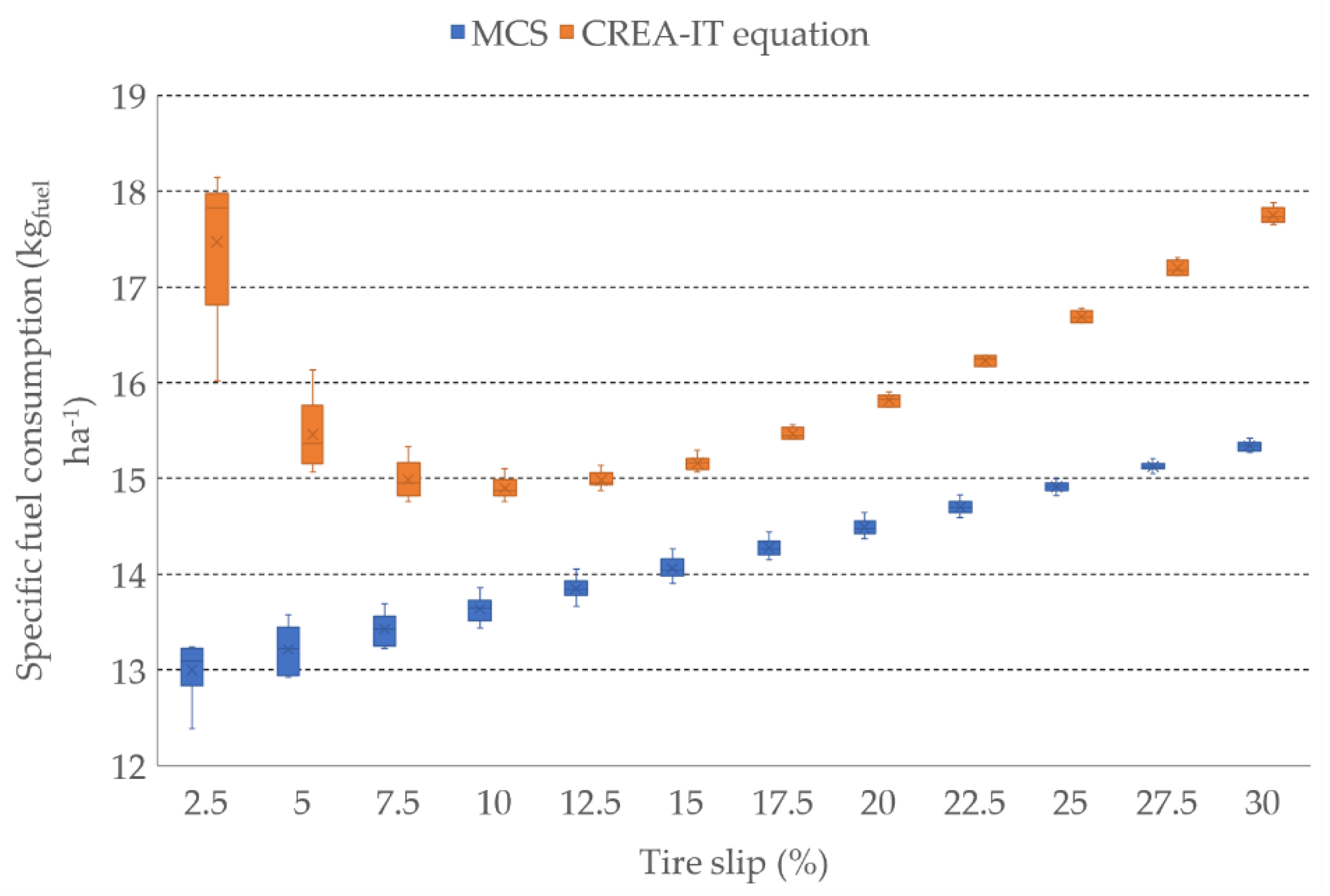
• $\overline{SF{C}_{ha}}$ is the specific fuel consumption of the drawbar power (kg ha⁻¹);
• SFC_db is the specific fuel consumption at the drawbar (g kWh⁻¹);
• h_ha are the hours of work required for one hectare;
• P_db was taken from Equation (1) after the field trials.

Table 3. Details of the factors adopted in the experimental test.

Fixed	Measured	Calculated	Dependent
Driveline efficiency (α)	Slip (s)	Power used for the vehicle’s displacement (Pvd)	Specific fuel consumption of the drawbar power (SFCdb)
Specific fuel consumption of the engine (SFCkW)	Forward speed ($\overrightarrow{v}$)	Drawbar power (Pdb)
	Vehicle’s mass (M)	Engine power (PPTO)
	Drawbar force (F)	Dynamic traction ratio (Tr)

summarizes the factors and variables used.

3. Results

3.1. Linear Regression and Monte Carlo Analysis

Figure 2 shows the overall output of the MCS. The simulated contemporary variation of the grip, wheel slip, and engine specific fuel consumption (1000 model runs) resulted in a MCS output (SFC_ha) ranging from 12.4 to 16.7 g_fuel ha⁻¹ with an average value of 14.2 g_fuel ha⁻¹, a standard deviation of ±0.72 g_fuel ha⁻¹, and a 95% confidence interval of ±0.045 g_fuel ha⁻¹.

Figure 3 displays the MCS output analysis: when the model output was related to input variable distributions, there was a weak relationship of SFC_ha with tire grip, a positive linear relationship with SFC_kw, and a nonlinear relationship with wheel slip.

Based on the model results, the lowest achievable SFC_ha (12.4 kg ha⁻¹) results from a slip value of around 13%, while the highest value of 16.7 kg ha⁻¹ relates to a wheel slip of around 28%. The algorithm also showed high values of SFC_ha with a low wheel slip (Figure 3): such a situation commonly occurs when an excessively heavy tractor is used to carry out a task.

The LRA provided a more formal investigation of the variables’ importance in lowering the model’s uncertainty. For the performed task, the correlation coefficient of the input variables with fuel consumption explains how well they relate to the MCS output (Table 2). The resulting equation, whose R² is 0.89, is (Equation (16)):

$$SF{C}_{ha}=0.538-1.739·Grip+0.052·SF{C}_{kW}+0.085·s$$

(16)

Table 4. Pearson correlation coefficients of the model inputs with the model output and the standardized regression coefficients resulting from the LRA.

Input Variable	Corr. Coeff. (r)	SRC
Grip (% net traction)	−0.15	−0.14
Wheel Slip (%)	0.73	0.60
SFCkW (gfuel kWh−1)	0.57	0.74

reports the SRCs for the equation above. The SRCs quantify the linear effect of the input variables on the dependent variable: their effectiveness is conditional on having a relatively high fit (R² = 0.89), which means that the regression model is relatively linear so that sensitivity analysis can be based on it [33].

In terms of the rank of the factors by importance depending on the absolute value of the SRCs, SFC_kW and Wheel slip were found to be the most influential variables among those studied. However, under operative conditions, SFC_kW is almost constant (it depends on the used machinery), and therefore, wheel slip is the most influential input variable.

3.2. The Experimental Trials: Effects of Different Tires on the Traction Efficiency

The measurement of the dynamic traction ratio of the tractor resulting from different sets of tires under field conditions resulted in the values displayed in Figure 4 (traction data expressed as the ratio of the drawbar pull (F) to the tire load (kN) normal to the surface (M) as a function of the slip). These drawbar pull tests confirmed reports in the literature showing that the drawbar pull increases nonlinearly with slip, and at higher slip values, the slope of the curve decreases towards 0.

Figure 5 reports the output of this assessment. It points out that the lowest SFC_db value (corresponding to the best drawbar power) occurred in the 7.5–12.0% range of wheel slip.

3.3. Validation

Figure 6 compares the outputs of the two processes undergone by the CREA-IT (SFC_ha from MCS and $\overline{SF{C}_{ha}}$ from the test trials) to calculate the specific fuel consumption (kg_fuel ha⁻¹). The field test outputs, processed with the CREA-IT equation, resulted in a mean fuel consumption per hectare, calculated with 10% slip, of 14.89 ± 0.12 kg ha⁻¹ [Equation (15)], which is in line with the output of the Monte Carlo simulation (13.64 ± 0.14 kg ha⁻¹, Equation (16)). These data confirm the assumptions of the MCS: the effect of the choice of tire on fuel consumption during heavy drawbar tasks has a maximal variation of 1% when performed at tire slip values higher than 10%.

Table 5. Squared error with varied slip levels.

Slip%	Squared Error
2.5	19.96
5	5.04
7.5	2.44
10	1.59
12.5	1.28
15	1.20
17.5	1.41
20	1.77
22.5	2.34
25	3.15
27.5	4.28
30	5.80

reports the squared error of the specific fuel consumption per hectare resulting from the comparison between the MCS and the CREA-IT equation. It shows that the best fit for the simulated output with the experimental results occurs for slip values between 10% and 20%.

4. Discussion

The studied variables relate to the tractor–implement combination chosen by a farmer in terms of the tractor mass and engine power. Increasing the weight of the tractor, on the one hand, decreases the power lost as slip, but on the other, increases the power lost through rolling resistance. The efficiency remains relatively stable at slip values of 7–15% but decreases exponentially at values under 5% (Figure 6). The effect of the slip value was shown to be significant in both the MCS and CREA-IT equations: on the one hand, the best fit among the curves occurred when the slip was in the 10–20% range and, on the other, the worst fit occurred at a low level of slip (<5%). This results from the averaging effect provided by the MCS process for the power used for the vehicle’s displacement (P_vd). Accounting for P_vd in the MCS process leads to the adoption of a quadratic model instead of a linear one.

When using a tractor with a mass and engine power slightly higher than ideal, the difference in efficiency is negligible, and it is easy for the operator to manage the engine load and speed (min⁻¹).

However, adopting a tractor smaller than the ideal or with a much higher mass and power than required will drastically decrease the efficiency. In the first case (Figure 7, on the left), having a tractor mass and power smaller than those required leads means that (i) there is high tire slip, (ii) the engine works at close to its maximum power level, and (iii) the small tire diameter does not result in a high tractive efficiency. In the second eventuality (the tractor mass and power are much higher than required, Figure 7, on the right), the mass of the tractor leads to (i) a high level of power loss due to rolling resistance and (ii) an inability to work at the correct engine load and speed (min⁻¹).

Practically, correct management of the slip follows the choice of the correct tractor mass and may affect fuel consumption by up to 20%.

Moreover, both uneven engine performance and overload or strain of the tractor’s engine should be avoided [20]. Therefore, a tractor with a reserve of power or torque is necessary and should ideally be equipped with a power management system. In fact, in the case of a tractor with a manual gearbox, keeping the engine at a reduced speed can be complicated. With a power-shift gearbox, it is possible to obtain the required engine power, but the ideal technical solution will result in the system continuously adapting to engine load and speed. Two methods allow such adaptation: adopting a continuously variable transmission (the operator sets the forward speed, and the tractor maintains it at a rate that is as constant as possible) or managing the engine curve (i.e., deciding on the unloaded engine rotation and then having a system that maintains the desired engine speed by varying the fuel injection). A combination of the two systems is also available in automatic mode.

In this simulation (moldboard plow, 1.8 m width, 0.3 m tillage depth, and 7 km h⁻¹ forward speed), the overall power required at the engine is 57.5 kW. Therefore, adopting an 87-kW power tractor with the tractor mass set at 5810 kg, providing a maximum power of 57.2 kW at 1200 min⁻¹, was enough to perform this task. However, even driving it at 1500 min⁻¹ (75 kW maximum power) would allow the performance of the task to be done while working under a partial load. In this case, the resulting specific fuel consumption would range between an ideal value of 245 g kWh⁻¹ (full load at 1200 min⁻¹) and 255 g kWh⁻¹ (partial load at 1500 min⁻¹).

5. Conclusions

This study presents a simplified approach based on the MCS to assess the key parameters related to the fuel consumption of agricultural tractors during heavy agricultural drawbar works. The study underlines and quantifies the importance of using a good tractor engine mass and wheel slip combination. Tractor setting (acting directly on the tire slip) and engine management greatly influence the specific fuel consumption per hectare (±15% range), while tire traction properties have minor influences on fuel efficiency.

The study confirms the importance of keeping tire slip close to 10%, which means that traction tests on agricultural tires also have to be carried out at comparable slip values (7–10%). Moreover, significant attention is required when measuring fuel consumption during implement or tire tests. Control of the settings at which the engine is used, such as speed and load, is fundamental to obtain comparable results. Tractors without engine control in economy mode may be inappropriate for fuel consumption comparisons during agricultural tasks.

References

1. OECD—Organisation for Economic Co-Operation and Development. Code 2: OECD Standard Codes for the Official Testing of Agricultural and Forestry Tractors Performance; OECD: Paris, France, 2018. [Google Scholar]
2. Molari, G.; Sedoni, E. Experimental evaluation of power losses in a power-shift agricultural tractor transmission. Biosyst. Eng. 2008, 100, 177–183. [Google Scholar] [CrossRef]
3. Harris, B.J.; Rethmel, B.R. Comparison of IF and standard marked metric radial ply tires. In Proceedings of the American Society of Agricultural and Biological Engineers Annual International Meeting, ASABE, Louisville, KY, USA, 7–10 August 2011; Volume 7, pp. 5461–5472. [Google Scholar]
4. Smerda, T.; Cupera, J. Tire inflation and its influence on drawbar characteristics and performance—Energetic indicators of a tractor set. J. Terramechanics 2010, 47, 395–400. [Google Scholar] [CrossRef]
5. Monteiro, L.A.; Albiero, D.; De Souza, F.H.; Melo, R.P.; Cordeiro, I.M. Tractor efficiency at different weight and power ratios. Rev. Cienc. Agron. 2013, 44, 70–75. [Google Scholar] [CrossRef]
6. Gil-Sierra, J.; Ortiz-Canavate, J.; Gil-Quiros, V.; Casanova-Kindelan, J. Energy efficiency in agricultural tractors: A methodology for their classification. Appl. Eng. Agric. 2007, 23, 145–150. [Google Scholar] [CrossRef]
7. Turker, U.; Ergul, I.; Eroglu, M.C. Energy efficiency classification of agricultural tractors in Turkey based on OECD tests. Energy Educ. Sci. Tecnol. Part A Energy Sci. Res. 2012, 28, 917–924. [Google Scholar]
8. Grisso, R.D.; Kocher, M.F.; Vaughan, D.H. Predicting tractor fuel consumption. Appl. Eng. Agric. 2004, 20, 553–561. [Google Scholar] [CrossRef]
9. Lacour, S.; Burgun, C.; Perilhon, C.; Descombes, G.; Doyen, V. A model to assess tractor operational efficiency from bench test data. J. Terramechanics 2014, 54, 1–18. [Google Scholar] [CrossRef]
10. Tiwari, V.K.; Pandey, K.P.; Pranav, P.K. A review on traction prediction equations. J. Terramechanics 2010, 47, 191–199. [Google Scholar] [CrossRef]
11. Pochi, D.; Fanigliulo, R.; Pagano, M.; Grilli, R.; Fedrizzi, M.; Fornaciari, L. Dynamic-energetic balance of agricultural tractors: Active systems for the measurement of the power requirements in static tests and under field conditions. J. Agric. Eng. 2013, 44, 415–420. [Google Scholar] [CrossRef]
12. Zoz, F.M.; Grisso, D.R. Tractor and Traction Performance. In Proceedings of the 2003 Agricultural Equipment Technology Conference, Louisville, KY, USA, 9–11 February 2003; ASAE Distinguished Lecture # 27; ASAE Publication Number 913C0403. ASAE: St. Joseph, MI, USA, 2003. [Google Scholar]
13. Lyasko, M.I. How to calculate the effect of soil conditions on tractive performance. J. Terramechanics 2010, 47, 423–445. [Google Scholar] [CrossRef]
14. Filho, A.G.; Lancas, K.P.; Leite, F.; Acosta, J.J.B.; Jesuino, P.R. Performance of agricultural tractor on three different soil surfaces and four forward speeds. Rev. Bras. Eng. Agrícola Ambient. 2010, 14, 333–339. [Google Scholar]
15. Cutini, M.; Brambilla, M.; Bisaglia, C. Tractor Drive Line Efficiency Evaluation taking into account Power Lost in Slippage. In Proceedings of the “New Engineering Concepts for Valued Agriculture”, Wageningen, The Netherlands, 8–12 July 2018; pp. 533–538. [Google Scholar]
16. Cutini, M.; Bisaglia, C. Development of a dynamometric vehicle to assess the drawbar performances of high-powered agricultural tractors. J. Terramechanics 2016, 65, 73–84. [Google Scholar] [CrossRef]
17. Prairie Agricultural Machinery Institute (PAMI). Research Update, Standardised Tractor Performance Testing. What It Is—And Isn’t; Prairie Agricultural Machinery Institute: Humboldt, SK, Canada, 1996. [Google Scholar]
18. ASAE D497.7; Agricultural Machinery Management Data. ASABE: St. Joseph, MI, USA, 2011.
19. Cutini, M.; Brambilla, M.; Bisaglia, C.; Pochi, D.; Fanigliulo, R. Efficiency of Tractor Drawbar Power Taking into account Soil-Tire Slippage. Lect. Notes Civ. Eng. 2020, 67, 409–417. [Google Scholar] [CrossRef]
20. Grisso, R.D. Gear Up and Throttle Down; Publication 442-450 (BSE-326P); Virginia Cooperative Extension, Virginia Tech: Blacksburg, VA, USA, 2001. [Google Scholar]
21. ASABE Standards S296.5 W/Corr. 1 DEC2003 (R2013); General Terminology for Traction of Agricultural Traction and Transport Devices and Vehicles. ASABE: St. Joseph, MI, USA, 2015.
22. EP496.3 FEB2006 (R2015); Agricultural Machinery Management. ASABE: St. Joseph, MI, USA, 2015.
23. Metropolis, N. The beginning of Monte Carlo methods. Los Alamos Sci. 1987, 15, 125–130. [Google Scholar]
24. Buc, D.; Màsàrova, G. Application of Monte Carlo simulation in the field of mechanical engineering. AD ALTA J. Interdiscip. Res. 2013, 3, 31–34. [Google Scholar]
25. Osaki, M.; Aparecido Alves, L.R.; Lima, F.F.; Garcia Ribeiro, R.; Sant’Ana de Camargo Barros, G. Risks associated with a double-cropping production system—A case study in southern Brazil. Sci. Agric. 2017, 76, 130–138. [Google Scholar] [CrossRef]
26. Colantoni, A.; Villarini, M.; Monarca, D.; Carlini, M.; Mosconi, E.M.; Bocci, E.; Hamedani, S.R. Economic analysis and risk assessment of biomass gasification CHP systems of different sizes through Monte Carlo simulation. Energy Rep. 2021, 7, 1954–1961. [Google Scholar] [CrossRef]
27. Briggs, A.; Goeree, R.; Blackhouse, G.; O’Brien, B. Probabilistic Analysis of Cost-Effectiveness Models: Choosing between Treatment Strategies for Gastro-Esophogeal Reflux Disease; Research Working Paper; McMaster University Centre for Health Economics and Policy Analysis: Hamilton, ON, Canada, 2001. [Google Scholar]
28. Qin, F.; Zhao, Y.; Shi, X.; Xu, S.; Yu, D. Sensitivity and uncertainty analysis for the DeNitrification–DeComposition model, a case study of modeling soil organic carbon dynamics at a long-term observation site with a rice–bean rotation. Comput. Electron. Agric. 2016, 124, 263–272. [Google Scholar] [CrossRef]
29. Clark, C.E. The PERT Model for the Distribution of an Activity Time. Oper. Res. 1962, 10, 405–406. [Google Scholar] [CrossRef] [Green Version]
30. Minitab, version 17; Statistical Software; Minitab: State College, PA, USA, 2010.
31. Campolongo, F.; Saltelli, A.; Sørensen, T.; Tarantola, S. Hitchhiker’s guide to Sensitivity Analysis. In Sensitivity Analysis; Saltelli, A., Chan, K., Scott, E.M., Eds.; John Wiley & Sons Ltd.: Hoboken, NJ, USA, 2000; pp. 16–45. [Google Scholar]
32. ENAMA Protocol n. 41. Pneumatici Per Ruote Motrici e Direttrici; ENAMA: Rome, Italy, 2000.
33. Saltelli, A.; Tarantola, F.; Campolongo, F.; Ratto, M. Sensitivity Analysis in Practice; Wiley: Hoboken, NJ, USA, 2004; ISBN 978-0-470-87093-8. Available online:http://www.andreasaltelli.eu/file/repository/SALTELLI_2004_Sensitivity_Analysis_in_Practice.pdf (accessed on 13 March 2022).
Figure 1. Example of the shape of the maximum PPTO and the relative SFCkW of a 71 kW tractor. A representation of the required power and the “ideal” working point in terms of efficiency is provided (i.e., 57 kW at 1400 min−1).
Agronomy 12 01017 g001
Figure 2. Percentage frequency distributions of the three random input variables (G, SFCkW, and s) and the output (SFCha) of the Monte Carlo Simulation.
Agronomy 12 01017 g002
Figure 3. Boxplots (highest and lowest data values, median, first and third quartiles) representing the distributions of the model output (SFCha) vs. the simulated wheel slip, tire grip, and the specific fuel consumption of the engine (SFCkW). Dots “·” represent outliers.
Agronomy 12 01017 g003aAgronomy 12 01017 g003b
Figure 4. Boxplots representing the dynamic traction ratio during tests carried out at various levels of slip (highest and lowest data values, median, first and third quartiles).
Agronomy 12 01017 g004
Figure 5. Boxplots representing the specific fuel consumption of the power at the drawbar during the tests carried out at various levels of slip (highest and lowest data values, median, first and third quartiles).
Agronomy 12 01017 g005
Figure 6. Comparison of the specific fuel consumptions (kgfuel ha−1) resulting from the Monte Carlo algorithm and the CREA-IT output.
Agronomy 12 01017 g006
Figure 7. Examples of incorrect coupling of the implement and the tractor size. The mismatch results in the inability to manage the operational parameters efficiently.
Agronomy 12 01017 g007