Water Accounting and Productivity Analysis to Improve Water Savings of Nile River Basin, East Africa: From Accountability to Sustainability

Abstract

Complete water accounting (WA) and crop water productivity (CWP) analysis is crucial for evaluating water use efficiency (WUE). This study aims to evaluate the contributions of hydro-meteorological factors to the changes of WA and CWP and subsequent WUE based on the data from 2009–2020 in the Nile River Basin (NRB), East Africa (EA). The Mann-Kendall (MK) statistical test and Sen’s slope estimator were applied to detect the trends of climatic factors, and the AquaCrop model was used to simulate the crop yields in response to water balance and consumption based on crop physiological, soil water, and salt budget concepts. For the years 2012 and 2019, the mean of climatic water deficit P − ETa was 71.03 km³ and 37.03 km³, respectively, which was expected to rise to ~494.57 km³ by 2050. The results indicated that the basin water budget was unbalanced due to the coupled impact of year-to-year hot and dry conditions and increase in water abstraction, an indication of water deficit or stress. CWP and WUE increased during the study period with different changing patterns. CWP was also found to correlate to the yield of major crops (p-value > 0.05). It was concluded that climatic factors influenced the crop yield, CWP, and WUE in the study area. Thus, the improvement of CWP and WUE should rely on advanced water-saving innovations. The findings of this study could help water managers to improve water productivity by focusing on water account potentials and creating regional advantages by deploying water in combination with surplus flow from upstream to downstream consumption.

1. Introduction

Water scarcity is an emerging global crisis; however, information useful for decision making related to water management seems to be lacking. Most importantly, little is known about information development over time [1,2]. To sustain food and water security today and in the future, water resources conservation faces critical challenges [3,4] including scarcity, waterlogging, depletion, increasing salinity, and coordination issues [5]. In 2050, food production is expected to meet the needs of a population of 9 to 10 billion people [6,7]. Subsequently, sufficient water is needed to produce the food. Practically, agriculture is one of the leading water users today and responsible for 70% of all freshwater withdrawal in the world, compared to 20% by industry and 10% by domestic use [8]. The 50% increase in agricultural production by the surging demand in 2050 compared to the 2013 baseline [9] exerts increased pressure on water quantity and quality. Therefore, improved crop water productivity (CWP), an assessment that quantifies sustainable agricultural water use and thereby inform economic policy and water accounting (WA), is needed. Predicting an attainable yield under coupled climate and water-limiting conditions is also a crucial goal in arid and drought-prone environments. The improvement allows for better managing water demand in agriculture [10,11], albeit integrated holistic approaches for water resource management are essential under global climate changes and regional economic and environmental problems [12,13]. Certainly, systematic monitoring helps to evaluate CWP gaps and identify appropriate solutions for closing these breaches while contributing directly to adaptive policy decisions and sustainable development goals (SDGs) (specifically SDG 2.3 on ending all forms of malnutrition, 2.4 on promoting sustainable food production systems and implementing resilient agricultural practices, and SDG 6.4 on improved water use efficiency).

The East Africa (EA) region, with its basins, dominated by the NRB, has some of the world’s largest water resources. The distribution of water varies significantly within the region [14]. The EA region is among the most environmentally diverse regions of the continent, as reflected in its ecosystem and hydrology [15,16]. The EA is a hydrological mosaic that has long influenced the social, cultural, and economic diversity of its human populations [17]. The spatial and uneven distribution (i.e., transboundary capitals) of water resources has created an upsurging water allocation and continuously increased competition between hydropower in the upstream and agriculture in the midstream and downstream areas [18], including the Grand Ethiopian Renaissance Dam (GERD) [19], Lake Victoria Basin [20,21], and Lake Tanganyika Basin [22]. Furthermore, several studies revealed the major shortcomings towards the usefulness and achievements of the NRB including poverty, poor infrastructure, environmental degradation, lack of overall strong political leadership and institutional framework, absence of agreement on water allocation among riparian nations, water resources conflicts, and doubts among the downstream and upstream states on water resource development [23,24,25].

Present concerns of water use in different areas of EA were raised by several researchers [26,27,28,29,30]. The attention of past studies was to enhance the water resources management by conserving the existing water sources, taming surface water use (i.e., irrigation), and improving agroecosystems water use efficiency (WUE) [31,32,33]. Currently, there have been few prior attempts to investigate CWP and WA in order to quantify how much water is used and saved for and from agricultural systems at different scales; consequently, further studies are suggested on the basin. Agricultural production should also be expressed in production per unit of water consumed or, in short CWP besides per unit of land (kg ha⁻¹). In this context, the vaporization of water from land into the atmosphere as well as water in the products produces agro-ecological-economical services. Further, coupled ‘‘traditional and modern’’ techniques of computing Real Water Savings (ReWaS) that focus on improving farm water consumption related activities or irrigation WUE help attain sustainable water resources management by adopting a variety of institutional policy reforms based on principles of scientific facts, participation, and sustainability (see also in Mozambique [34], Nepal [35], and Vietnam [36] for similar points of view). Careful monitoring of CWP in agriculture and exploring opportunities to increase the WUE are thus essential in agricultural practices.

Given the role of agricultural systems in confronting the challenge of eradicating hunger and improving food and water security [37], maintaining a sustainable supply of water resources to meet these demands is a major water management challenge for the Nile region due to the increasing population and water demand, recurring drought, and climate change [38]. Specifically, the purpose of this study is to (1) assess the long-term trends in climatic factors in the NRB; (2) examine the seasonal CWP of major crops; and (3) analyze the WA and water-saving potentials of the NRB. This study established a comprehensive technique to quantify water savings and applied this technique in the NRB. By relying on CWP and WA, the method used in this study considered biomass production, evapotranspiration, evaporation, interception, transpiration, and other influencing factors, which helped irrigation managers to find ways to improve the WUE by decreasing the ratio of evaporation to transpiration. In this paper, the argument was also extended to explore the future policy implications for agricultural research. The outcomes of this study are crucial in the overall management of the NRB as well as in the other arid and semi-arid areas that experience water losses and scarcity.

2. Materials and Methods

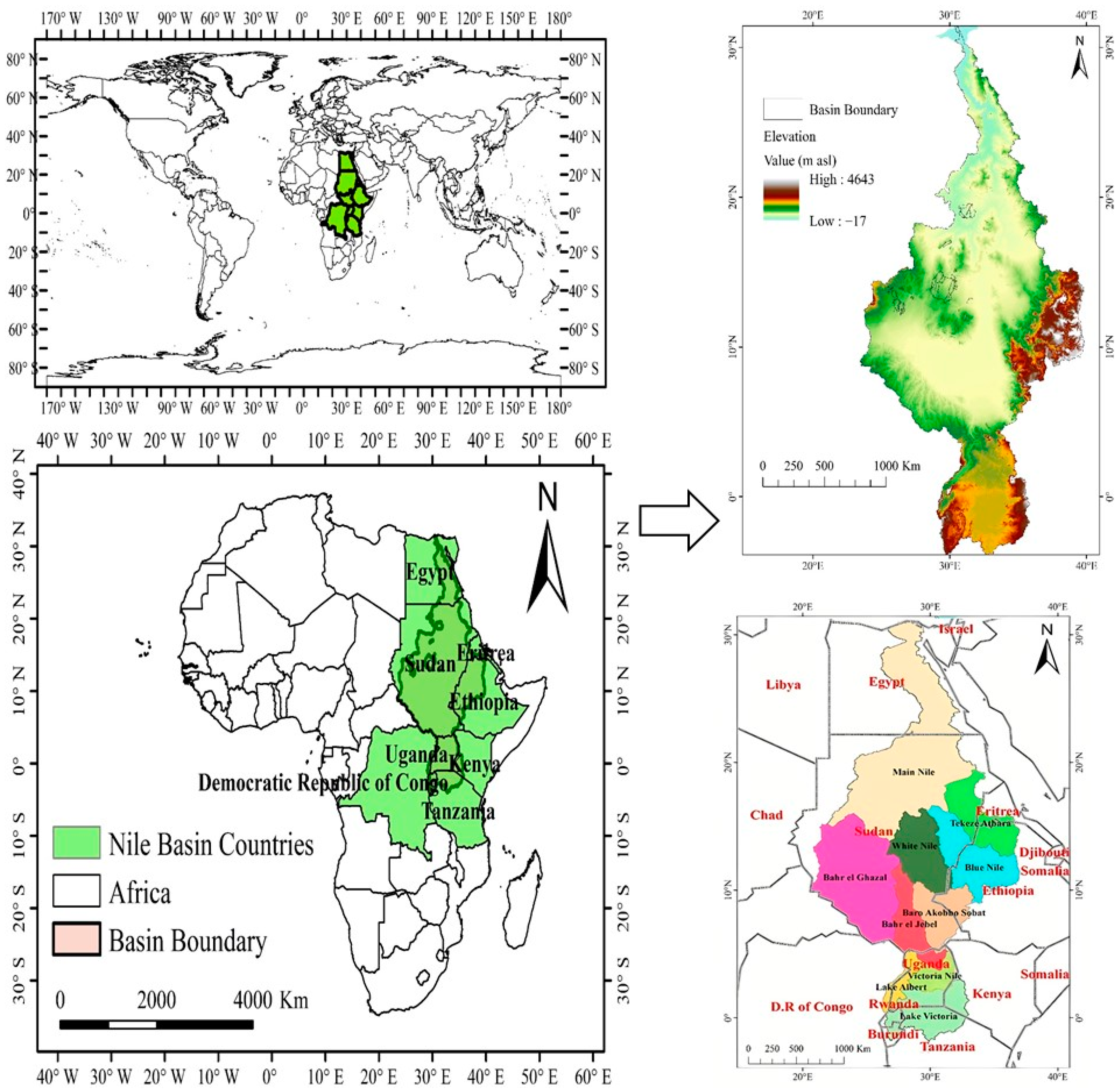
2.1. Study Area

The Nile River (NR), as one of the most important water suppliers of freshwater in the Mediterranean Sea, flows from south to north through eastern Africa. The NR is also the longest river in the world, running ~66,800 km of length while snaking through 11 riparian countries—Ethiopia (1,100,000 km²), Sudan (1,886,068 km²), South Sudan (644,329 km²), Egypt (1,001,450 km²), Rwanda (26,338 km²), Tanzania (945,087 km²), Uganda (241,037 km²), Burundi (27,834 km²), the Democratic Republic of Congo (DRC) (2,344,858 km²), Eritrea (117,600 km²), and Kenya (580,367 km²) (Figure 1). NR extends over a wide range of latitudes (4° S–31° N), and the major sources are Lake Victoria (~68,800 km²) in east-central Africa. The White Nile flows North through Uganda, eventually crossing into Sudan where it intersects the Blue Nile at Khartoum, which originates in the Ethiopian highlands [39]. The Nile runs through highland regions with abundant moisture to lowlands with 4 differentiated aridity conditions (i.e., moist sub-humid, dry sub-humid, semi-arid, and arid zones). The Nile and its ecosystem are complex, splitting into many sub-basins each with different hydro-biogeochemical characteristics [40]. The areas that contribute to the total flow—the equatorial lakes plateau regions, e.g., Lake Victoria, located in modern-day Uganda, Tanzania, and Kenya, Lake Tana in Ethiopia, and the Ethiopian massifs are relatively small and isolated. According to Ainsworth et al. [41], the overexploitation of the NRB has resulted in a significant decrease in the watercourses. Meanwhile, a large volume of run-off is generated in different regions, most of which is lost due to evaporation from wetlands, channel losses, and human abstraction via agrarian purposes [42].

The NRB covers ~3,028,230.55 km² (

Table 1. NR sub-basins and their drainage area.

No	Sub-Basin	Area
		km2
1	Equatorial Lake Basin	394,147.06
2	Upper White Nile	234,680.83
3	Bahr-el-Ghazal	584,199.81
4	Baro-Akobo-Pibor-Sobat	206,418.15
5	Lower White Nile	256,040.61
6	Blue Nile	298,382.84
7	Tekeze-Atibara-Setite	221,685.09
8	Main Nile upstream of Dongola	389,105.60
9	Main Nile downstream of Dongola	443,570.58
Total area		3,028,230.55

) shared from eastern-north Africa, about 10% of the area of Africa [40]. The coverage region experiences extreme climatic fluctuations. This region covers broadly different climatic zones such as arid, temperate, and tropical zones [44] with a typical continental climate. The interannual distribution of runoff is uneven, and the outflow (only ~13 km³·year⁻¹) is relatively small compared to its size [45] due to ~50–85% loss in the flows of the White Nile at the basin interstation that includes the Sudd wetlands in South Sudan [46]. NR is the only and daily water source for a big population. Specifically, NR supplies water to ~4 × 10⁸ people and more than 50% of the population live within the NRB [47,48]. The hydrological infrastructures that control the water in the NRB include dams and reservoirs. For example, the Aswan High Dam reservoir (~6000 km², 162 km³) and Grand Ethiopian Renaissance Dam (GERD) reservoir (~1874 km², 74 km³) are located upstream in Egypt and Ethiopia, respectively. Based on the per capita gross domestic product (GDP) at purchasing power parity, this region is characterized by low average incomes. This fact, in addition to the dependence of national economies on the agricultural sector in terms of GDP and employment, makes climatic conditions and particularly rainfall a crucial issue for social and economic development [49].

Within the NRB, there are four generalized types of hydrogeological environments: crystalline/metamorphic basement rocks, volcanic rocks, unconsolidated sediments, and consolidated sedimentary rocks [50]. A portion of groundwater use in the NRB includes domestic water supply in rural and urban settings for drinking and household use, as well as small commercial activities; industrial use and tourism development; agricultural use for irrigation and livestock production from subsistence through to commercial scales; and large-scale industrial activities, such as mineral exploitation. For instance, over the last 40 years, increasing groundwater demand has considerably impacted the Nubian Sandstone Aquifer System (NSAS), resulting in the loss and shrinkage in water of several springs and oasis (e.g., the case of Kharga Oasis) [51,52]. Almost half of the NRB countries are projected to live below the water scarcity level of 1000 m³·person⁻¹·year⁻¹ by 2030 due to factors such as doubling rural and urban population growth [53]. From 2009 to 2020, the cropland increased in NRB countries while the forest land decreased (Figure 2 and

Table 2. Land-use variation in the NRB countries from 2009–2020.

	Area (km2)					Area (km2)					Area Change
	2009					2020					2009–2020
Country	PMP	CP	AG	FL	OL	PMP	CP	AG	FL	OL	PMP	CP	AG	FL	OL
BUR	483	1350	193.9	1867	507.1	483	1550	279.6	2033	255.4	0	200	85.7	166	−251.7
DRC	50	2630	143,899	25,600	57,206	50	2580	127,256.6	31,500	67,948.4	0	−50	−16,642.4	5900	10,742.4
EGY	0	3671	59.2	3291	96,194.8	0	3836	45	3836	95,664.1	0	165	−14.2	545	−530.7
ERT	6900	692	1118.5	7530	1451.5	6900	692	1058.4	7592	3467.4	0	0	−60.1	62	2015.9
ETH	20,000	15,683	18,528.5	30,662	50,809.5	20,000	17,903	17,141.5	37,903	57,811.6	0	2220	−1387	7241	7002.1
KEN	21,300	6020	3961.2	26,671	26,281.8	21,300	6330	3611.1	27,630	25,672.9	0	310	−350.1	959	−608.9
RWA	430	1373.9	287	1670	510	410	1401.7	275	1811.7	380.3	−20	27.8	−12	141.7	−129.7
SSD	25,773.2	2618.9	7157	28,251	27,784.9	25,773.2	2477.7	7157	28,251	27,784.9	0	−141.2	0	0	0
SUD	48,195	19,991.2	18,531.7	68,186.2	98,205.5	48,195	19,991	18,531.7	68,186	98,205.5	0	0	0	0	0
TZN	24,000	13,450	53,670	34,000	4306.1	24,000	15,650	46,214	39,650	2716	0	2200	−7456	5650	−1590.1
UGA	5315	8950	3163	12,512	910	5315	9100	2379.2	14,415	3257.9	0	150	−783.8	1903	2347.9

Note: PMP: Permanent meadows and pastures, CP: Cropland, AG: Agricultural land, FL: Forest land, and OL: Other lands. NRB countries (BUR: Burundi, DRC: Democratic Republic of Congo, EGY: Egypt, ERT: Eritrea, ETH: Ethiopia, KEN: Kenya, RWA: Rwanda, SSD: South Sudan, SUD: Sudan, UGA: Uganda, TZN: Tanzania). The negative values indicate the decrease in land-use area.

). Any future changes in the magnitude of the flow volume of the NR can lead to significant impacts on the lives of people living within the basin [54].

2.2. Datasets

CWP is a simple function of crop production processes and water supplied to the crop, whereas the WUE is a ratio of grain yield produced per water consumed by the crop. The effectiveness of water productivity and water-saving accounts assessment considered different hydrometeorological indicators, as shown in Figure 3.

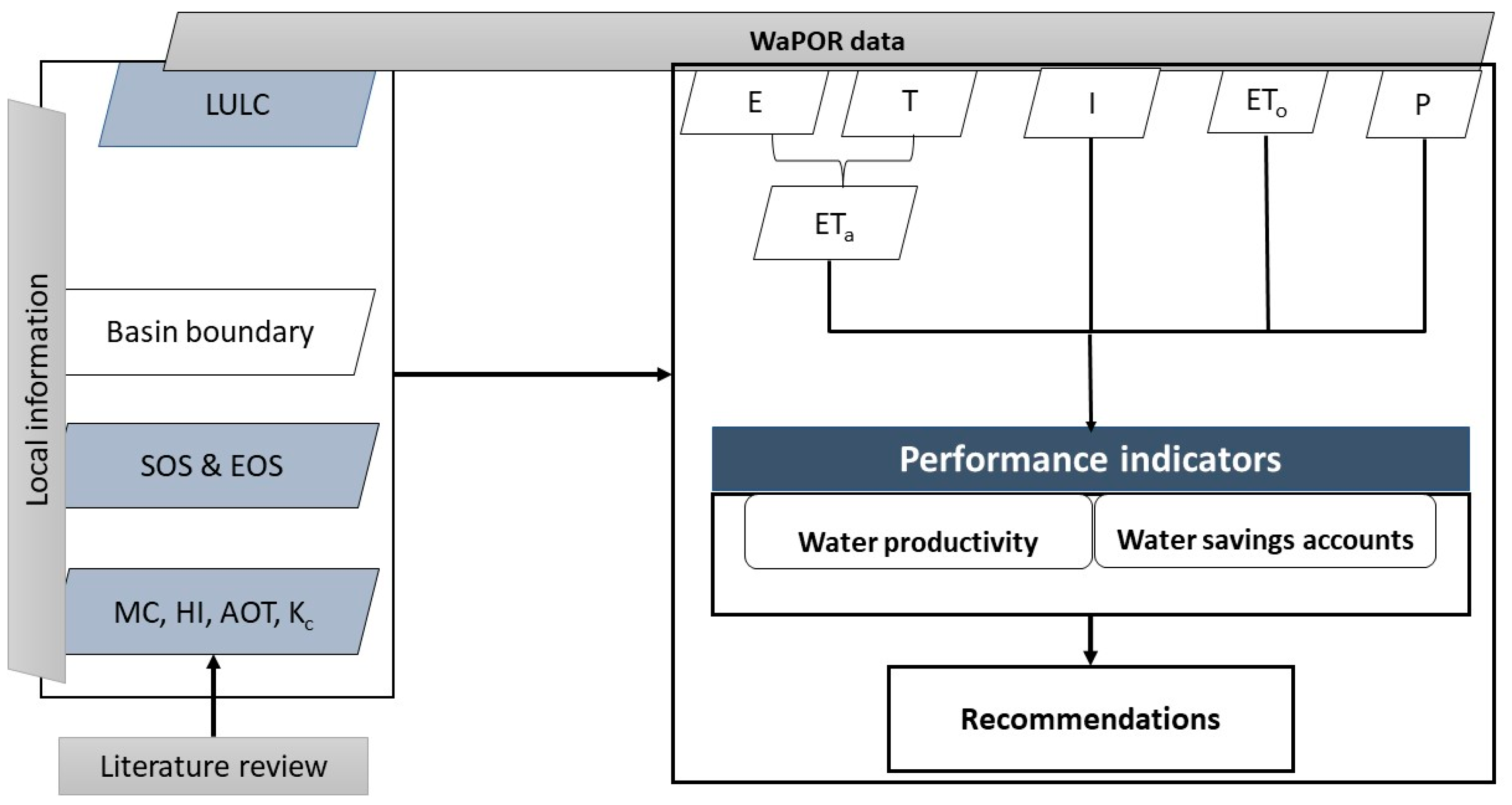
2.2.1. WaPOR Dataset

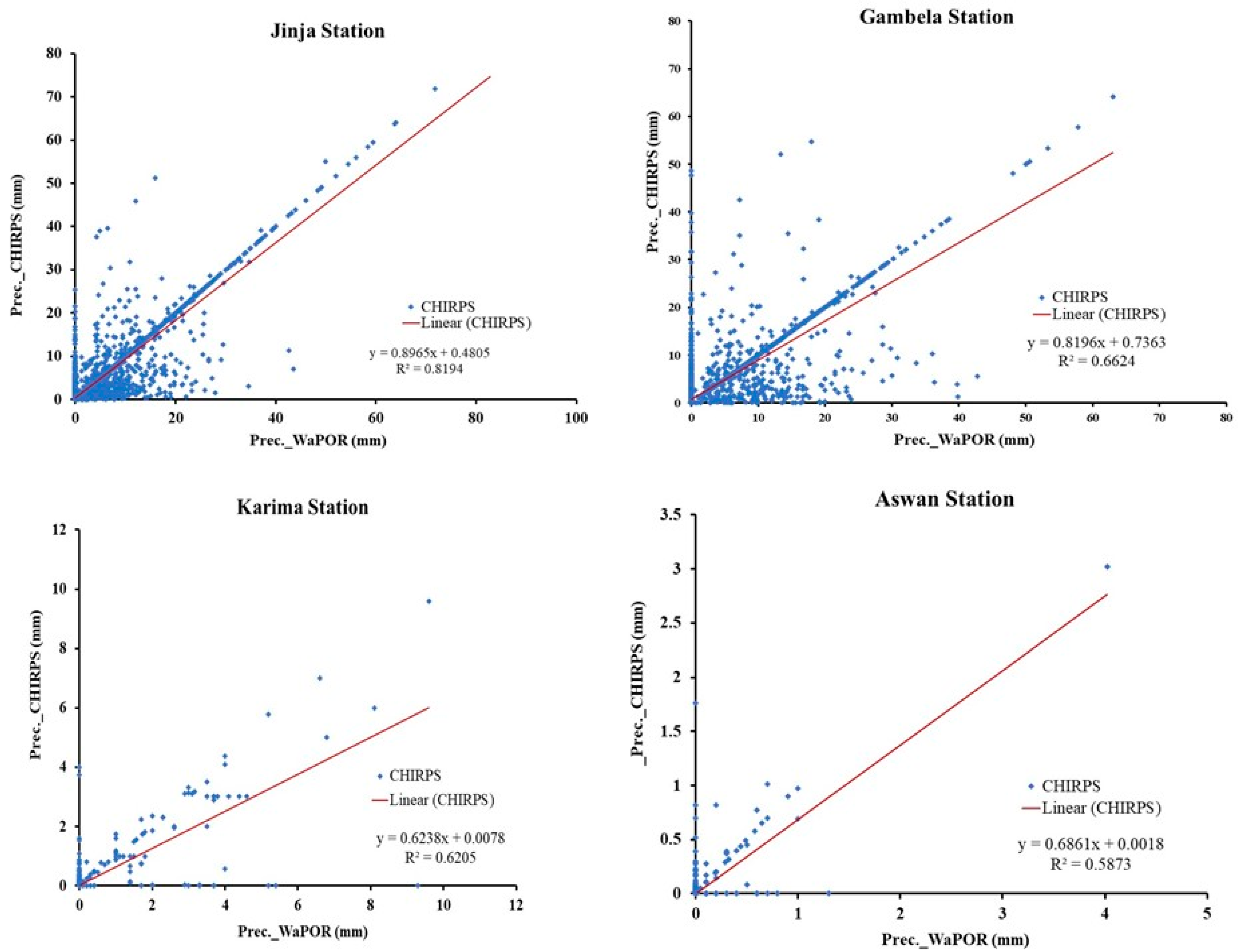
The Water Productivity through the Open access Remotely sensed derived data (WaPOR) dataset, developed by FAO, IHE Delft, and ITC, open-access data portal (WaPOR; https://wapor.apps.fao.org/home/WAPOR_2/1 (accessed on 6 December 2021)) was used for the analyses, which provided the required layers to estimate water productivity to more than 11 years. The WaPOR v2.1. database released in June 2019 was used for this study, which covered Africa and the Near East regions in near real-time for the period between 2009 to now [55]. WaPOR datasets are available at the continental scale (Level 1 at 250 m), country (Level 2 at 100 m), and project level (Level 3 at 30 m) [56,57]. The WaPOR v2.1 was found suitable for inter-plot comparison and large plots (>2 ha) [58]. For the NRB in East Africa, the finest resolution of the WaPOR data was 250 m (Level 1). The WaPOR Level 1 datasets used in this study included layers for precipitation (P), evaporation (E), actual evapotranspiration (ETa), actual evapotranspiration and interception (ETIa), transpiration (T), and interception (I) at annual and monthly timescales.

A synopsis of the WaPOR dataset used for this study is presented in Figure 3. The water accounting and water productivity assessment indicators were summarized in four main stages: (1) data collection, error measurement removal, extrapolation by statistical analysis using historical trends for a specified period, and graphical representation of the extrapolation results. The basin and its boundaries were delineated after land cover classification (LCC). Further, the moisture content (MC), harvest index (HI), above over total biomass (AOT), crop coefficient (Kc), the start of the season (SOS), end of the season (EOS), and other factors were investigated using the official published documents [59]; (2) water balance of the basin ($\mathrm{P}-{\mathrm{ET}}_{\mathrm{a}}$ $\iff$ ${\mathrm{ET}}_{\mathrm{a}}=\mathrm{E}-\mathrm{T}$); (3) water use evaluation for water accounting and productivity indicators assessment in the basin; and (4) recommendations from the analysis.

2.2.2. Climate Data

The precipitation (P) data were collected from the Climate Hazards Group InfraRed Precipitation with Station (CHIRPS), a 35+ year quasi-global rainfall dataset spanning 50° S–50° N (and all longitudes) at 0.05° × 0.05° spatial resolution, from 1981 to the near present, using in situ meteorological stations to create gridded rainfall time series for trend analysis [60]. These CHIRPS data are annually, monthly, and daily freely available at http://chg.geog.ucsb.edu/data/chirps/ (accessed on 21 November 2021). Each pixel contains a value that represents the total daily precipitation in the year in mm (1 mm = 1 L·m⁻² or 1 mm = 10 m³·ha⁻¹).

2.2.3. GRACE Dataset

This study considered the Gravity Recovery and Climate Experiment (GRACE) dataset, a dual-satellite mission continuously monitoring and mapping Earth’s changing gravity field to estimate the total water storage anomalies (TWSA) [61]. GRACE has multiple ways for estimating TWSA using gravity anomalies that cover the entire planet from 2003 to 2015. The data were downloaded freely from http://grace.jpl.nasa.gov/data/get-data (accessed on 7 November 2021). As a result, the GRACE system offers mean monthly TWSA because the number of days may not exactly match the days of the months and, as such, the change in storage ($\mathsf{\Delta }\mathrm{S}/\mathsf{\Delta }\mathrm{t}$) in a time period was approximated using a second-order central difference as described by Biancamaria et al. [62] At this time, the P − ET_a should be equal to the total outflow (OF), after correction in the change of storage with time.

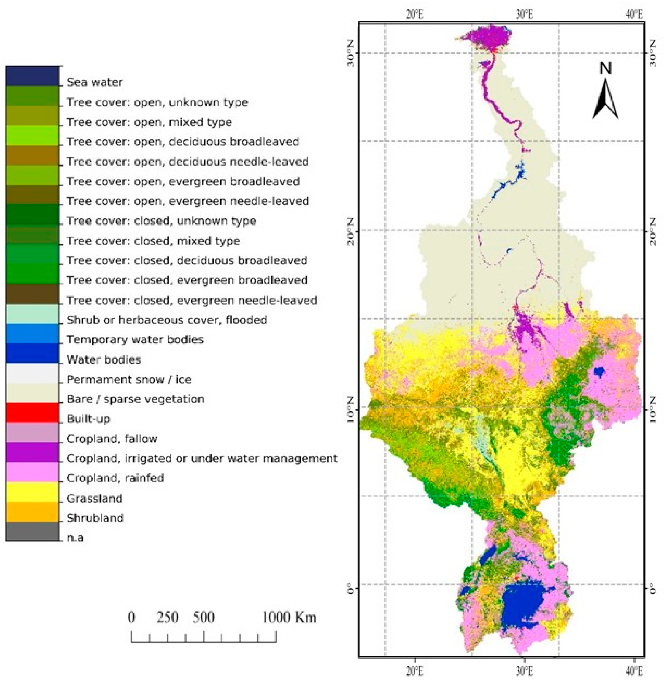
2.2.4. Land Cover Pattern Data

Annual data of the Level 1 land cover pattern were derived from the Global Land Service of Copernicus (GLSC) and the Earth Observation Programme (EOP) of the European Commission (EU) from 2009 to 2020. A static land map was employed to identify crop areas and assess the role of seasonal land-use dynamics. Water used by diverse crops was estimated by taking into account seasonal cumulative values precipitation-evapotranspiration (P − ET) in the whole basin. The global CGLS-100 m land cover map of 2015 served as a base layer for both Level 1 and 2, and the cropland class was further divided into irrigated, rainfed, and fallow on an annual basis. The classification was based on the Land Cover Classification System (LCCS) developed by the Food and Agriculture Organization (FAO) [63,64].

2.2.5. Data Validation

The relationship between precipitation (P; CHIRPS derived data) and WaPOR derived data at four meteorological stations (Appendix A,

Table A1. Country, meteorological station name, latitude, longitude, elevation, and time recorded.

Country	Station Name	Latitude	Longitude	Elevation	Time Recorded
		° N	° E	m asl	Year
Uganda	Jinja	0.45	33.15	1138.51	2009–2020
Gambela	Ethiopia	8.25	34.57	463.75	2009–2020
Karima	Sudan	18.55	31.85	308	2009–2020
Aswan	Egypt	23.97	32.78	463.75	2009–2020

) during 2009–2020 was shown in Figure 4. In general, the CHIRPS derived showed a high correlation (R²) of 0.81, 0.66, 0.62, and 0.56 for Jinja, Gambela, Karima, and Aswan station, respectively. The data showed good consistency between two different datasets used. Recent studies concluded that CHIRPS data can be employed to investigate the hydrologic impacts of low precipitation and high-temperature trends in Eastern Africa [59,65].

2.3. Methods

2.3.1. Description of Models

ETLook Model

The method to estimate the evaporation (E) and transpiration (T) data in WaPOR is built on the ETLook model as described by Bastiaanssen et al. [66], which uses the Penman-Monteith (P-M) equation [67], adapted to the geospatial data input. Using widely recorded meteorological data, the P-M equation estimates the rate of total evaporation and transpiration (air temperature, solar radiation, vapour pressure, and wind speed) [55]. The P-M equation (Equation (1)) is expressed as follows:

$$\mathsf{\lambda }\mathrm{ET}=\frac{\Delta \left({\mathrm{R}}_{\mathrm{n}}-\mathrm{G}\right)+{\mathsf{\rho }}_{\mathrm{a}}{\mathrm{C}}_{\mathrm{p}}\frac{\left({\mathrm{e}}_{\mathrm{s}}-{\mathrm{e}}_{\mathrm{a}}\right)}{{\mathrm{r}}_{\mathrm{a}}}}{\Delta +\mathsf{\gamma }\left(1+\frac{{\mathrm{r}}_{\mathrm{s}}}{{\mathrm{r}}_{\mathrm{a}}}\right)}$$

(1)

where $\mathsf{\lambda }$ is latent heat of evaporation (J·kg⁻¹), $\mathrm{E}$ is evaporation (kg m⁻²s⁻¹), $\mathrm{T}$ is transpiration (kg·m⁻²s⁻¹), ${\mathrm{R}}_{\mathrm{n}}$ is the net radiation (W·m⁻²), G is soil heat flux (W·m⁻²), ${\mathsf{\rho }}_{\mathrm{a}}$ is air density (kg·m⁻³), ${\mathrm{C}}_{\mathrm{p}}$ is specific heat of dry air (J·kg⁻¹·K⁻¹), ${\mathrm{e}}_{\mathrm{a}}$ is actual vapour pressure (Pa), ${\mathrm{e}}_{\mathrm{s}}$ is saturated vapour pressure (Pa), which is a function of air temperature, $\Delta$ the slope of the saturation vapour pressure vs. temperature curve (Pa·K⁻¹), $\mathsf{\gamma }$ is psychrometric constant (Pa·K⁻¹), ${\mathrm{r}}_{\mathrm{a}}$ is aerodynamic resistance (s·m⁻¹), and ${\mathrm{r}}_{\mathrm{s}}$ is bulk surface resistance (s·m⁻¹).

The ETLook algorithm employs a two-layer approach including the canopy transpiration (T) (Equation (2)) and soil evaporation (E) (Equation (3)) to solve the P-M equation, which is expressed as follows:

$$\mathsf{\lambda }\mathrm{T}=\frac{\Delta \left({\mathrm{R}}_{\mathrm{n},\mathrm{canopy}}-\mathrm{G}\right)+{\mathsf{\rho }}_{\mathrm{a}}{\mathrm{C}}_{\mathrm{p}}\frac{\left({\mathrm{e}}_{\mathrm{s}}-{\mathrm{e}}_{\mathrm{a}}\right)}{{\mathrm{r}}_{\mathrm{a},\mathrm{canopy}}}}{\Delta +\mathsf{\gamma }\left(1+\frac{{\mathrm{r}}_{\mathrm{s},\mathrm{canopy}}}{{\mathrm{r}}_{\mathrm{a},\mathrm{canopy}}}\right)}$$

(2)

$$\mathsf{\lambda }\mathrm{E}=\frac{\Delta \left({\mathrm{R}}_{\mathrm{n},\mathrm{soil}}-\mathrm{G}\right)+{\mathsf{\rho }}_{\mathrm{a}}{\mathrm{C}}_{\mathrm{p}}\frac{\left({\mathrm{e}}_{\mathrm{s}}-{\mathrm{e}}_{\mathrm{a}}\right)}{{\mathrm{r}}_{\mathrm{a},\mathrm{soil}}}}{\Delta +\mathsf{\gamma }\left(1+\frac{{\mathrm{r}}_{\mathrm{s},\mathrm{soil}}}{{\mathrm{r}}_{\mathrm{a},\mathrm{soil}}}\right)}$$

(3)

Therefore, the two Equations (2) and (3) differ with respect to the net available radiation $({\mathrm{R}}_{\mathrm{n},\mathrm{canopy}}$and ${\mathrm{R}}_{\mathrm{n},\mathrm{soil}}$) as well as the aerodynamic and surface resistance (${\mathrm{r}}_{\mathrm{a},\mathrm{canopy}}$, ${\mathrm{r}}_{\mathrm{s},\mathrm{canopy}}$, and ${\mathrm{r}}_{\mathrm{a},\mathrm{soil}}$, ${\mathrm{r}}_{\mathrm{s},\mathrm{soil}}$). Moreover, the soil heat flux (G) is not taken into account for transpiration.

AquaCrop Model

The AquaCrop model is among the most effective and frequently used crop yield (CY), CWP, and WUE simulation models [68]. The model simulates herbaceous crop yields based on transpiration losses [69]. It is a water-driven model because, in the growth engine, transpiration is converted into biomass by using biomass water productivity, conservative crop parameters, normalized for atmospheric evaporation and CO₂ concentration [70], as expressed in Equation (4).

$${\mathrm{B}}_{\mathrm{n}}={\mathrm{WP}}^{*}\times {{\displaystyle \sum }}_{\mathrm{i}=1}^{\mathrm{n}}\left(\frac{{\mathrm{T}}_{\mathrm{ri}}}{{\mathrm{ET}}_{\mathrm{oi}}}\right)$$

(4)

where ${\mathrm{B}}_{\mathrm{n}}$ is cumulative aboveground biomass production after $\mathrm{n}$ days (g·m⁻²), ${\mathrm{T}}_{\mathrm{ri}}$ is daily crop transpiration (mm·day⁻¹), ${\mathrm{ET}}_{0\mathrm{i}}$ is daily reference evapotranspiration (mm·day⁻¹), $\mathrm{n}$ is consecutive days of the period when biomass is produced, and ${\mathrm{WP}}^{*}$ is the normalized (g·m⁻²). When the mineral nutrients and water are not limiting factors in extremely severe cases, the ${\mathrm{WP}}^{*}$ is nearly constant for a specific crop.

2.3.2. Hydrometeorological Trend Analysis

The Mann–Kendall (MK) trend test is drawn on the correlation between the ranks and sequences of a time series [71,72]. It is widely used in detecting trends of variables in agrometeorological and hydrological indicators [73]. For a given time series $\left({\mathrm{X}}_{\mathrm{i},}\mathrm{i}=1,2\dots ,\mathrm{n}-1\right)$, the null hypothesis ${\mathrm{H}}_0$ assumes that it is independently distributed, and the alternative hypothesis ${\mathrm{H}}_1$ assumes that there exists a monotonic trend. The test statistic S can be obtained by Equation (5).

$$\mathrm{Y}={{\displaystyle \sum }}_{\mathrm{i}=1}^{\mathrm{n}-1}{{\displaystyle \sum }}_{\mathrm{j}=\mathrm{i}+1}^{\mathrm{n}}\mathrm{sgn}({\mathrm{X}}_{\mathrm{j}}-{\mathrm{X}}_{\mathrm{i}})$$

(5)

where ${\mathrm{X}}_{\mathrm{i}}$and ${\mathrm{X}}_{\mathrm{j}}$are the values of sequence i, j; n is the length of the time series and

$$\mathrm{sgn}\left({\mathrm{X}}_{\mathrm{j}}-{\mathrm{X}}_{\mathrm{i}}\right)=\{\begin{array}{c}+1, \mathrm{if} \left({\mathrm{X}}_{\mathrm{j}}-{\mathrm{X}}_{\mathrm{i}}\right) \mathrm{x}>0\\ 0, \mathrm{if} \left({\mathrm{X}}_{\mathrm{j}}-{\mathrm{X}}_{\mathrm{i}}\right) \mathrm{x}=0\\ -1, \mathrm{if} \left({\mathrm{X}}_{\mathrm{j}}-{\mathrm{X}}_{\mathrm{i}}\right) \mathrm{x}<0\end{array}$$

(6)

According to Kendall [72] and Mann [71], the statistic Y is approximately normally distributed when $\mathrm{n}\ge 8$ with the mean and variance of statistics of Y as follows:

$$\mathrm{E}\left(\mathrm{Y}\right)=0$$

(7)

$$\mathrm{V}\left(\mathrm{Y}\right)=\frac{\mathrm{n}\left(\mathrm{n}-1\right)\left(2\mathrm{n}+5\right)}{18}$$

(8)

Then the standardized test statistic Z is computed by Equation (9).

$$\mathrm{Z}=\{\begin{array}{c}\frac{\mathrm{Y}-1}{\sqrt{\mathrm{V}\left(\mathrm{Y}\right)}}, \mathrm{Y}>0\\ 0 \mathrm{Y}=0\\ \frac{\mathrm{Y}+1}{\sqrt{\mathrm{V}\left(\mathrm{Y}\right)}}, \mathrm{Y}<0\end{array}$$

(9)

The standardized MK statistic Z follows the standard normal distribution with E(Z) = 0 and V(Z) = 1, and the null hypothesis is rejected if the absolute value of Z is larger than the theoretical value Z_1−α/2 (for the two-tailed test) or Z_1−α (for the one-tailed test), where α is the statistical significance level concerned. If $\mathrm{Z}>0$, it indicates an increasing trend and vice versa. Given a confidence level α, the sequential data are supposed to experience a statistically significant trend if |Z| > Z(1 − α/2), where Z(1 − α/2) is the corresponding value of P = α/2 following the standard normal distribution. In this study, 0.05 and 0.01 confidence levels were used.

In addition, the magnitude of a time series trend was evaluated by a simple non-parametric procedure developed by Sen [74]. The trend is calculated by Equation (10).

$$\mathsf{\beta }=\mathrm{Median}\left(\frac{{\mathrm{X}}_{\mathrm{j}}-{\mathrm{X}}_{\mathrm{i}}}{\mathrm{j}-\mathrm{i}}\right),\mathrm{j}>\mathrm{i}$$

(10)

where $\mathsf{\beta }$ is Sen’s slope estimate. $\mathsf{\beta }>0$ indicates upward trend in a time series. Otherwise, the data series presents a downward trend during the time period.

2.3.3. Climatic Water Deficit (CWD) Calculation

The CWD approach is based upon a Thornthwaite water balance model [75]. The CWD is calculated on a time series basis as a difference between reference evapotranspiration (ET₀) and precipitation (P) in the following, Equation (11).

$$\mathrm{CWD}=\mathrm{P}-{\mathrm{ET}}_0$$

(11)

where P refers to the P (mm) and ET₀ (mm) to the study period, with monthly values.

The difference value of potential evapotranspiration and precipitation (P$-$ET) is negative when there is a severe water deficit, while a positive P$-$ET value represents a potential water surplus. If the P$-$PE value is less than zero, the month is called a “dry month”, and P$-$PE is equivalent to the accumulated potential loss (APWL) value. If the P$-$ET value is greater than zero, the month is called a “wet month”, and P$-$PE is equivalent to the surplus value. When the P > PE, it means that the soil is saturated from the excess precipitation. Hence, the ETa equals the PET because there are no changes to the soil moisture. When the P < PE, it means there are changes in the soil moisture. Thus, the actual evapotranspiration (ETa) equaling the P is subtracted by the changes in the soil moisture.

2.3.4. Water Balance Assessments

The water balance or budget (WB) is estimated based on the principle of mass conservation [76]. In this study, we followed the Molden and Sakthivadivel (M–S) procedure, which is based on a WB approach that combines groundwater and surface water as a single domain [77]. This study used a WB approach of the defined three-dimensional area over the specific time to derive the water accounts and productivity. Thus, the WB can be expressed as

$${\mathrm{P}}_{\mathrm{t}}={\mathrm{Q}}_{\mathrm{t}}+{\mathrm{E}}_{\mathrm{t}}+/-\mathsf{\Delta }\mathrm{S}$$

(12)

where ${\mathrm{P}}_{\mathrm{t}}$ refers to the precipitation $\left[\mathrm{mm}·{\mathrm{year}}^{-1}\right]$ from the study area in the year t, ${\mathrm{Q}}_{\mathrm{t}}$ refers to discharge or runoff $\left[\mathrm{mm}·{\mathrm{year}}^{-1}\right]$ of the study area in the year t, ${\mathrm{E}}_{\mathrm{t}}$ is the evaporation from the study area in the year t, and $\mathsf{\Delta }\mathrm{S}=\mathrm{dS}/\mathrm{dt}$refers to the storage changes per time step $\left[\mathrm{mm}·{\mathrm{year}}^{-1}\right]$.

The net inflow equals the gross inflow plus or minus the change in the storage. Water is consumed via evaporation and transpiration. The outflow of water is subdivided into commitment for downstream use, utilization either within the water accounting domain or somewhere else in the river, or depleted, when water is directed to a sink outside the domain.

2.3.5. Water Accounting (WA) Approach

The WA is the systematic acquisition, analysis, and dissemination of data on stocks and fluxes of water (from source to sinks) in natural, disturbed, or extensively managed settings [78]. Through WA, changes in water use (WU) patterns are analyzed [77]. The WA framework differentiates the various flows that are associated with WU and can be applied to any sector at any scale without modification. The WU is the application of water to a selected purpose (i.e., irrigation, industrial processes and among others). Typical recoverable flow fractions are between 20% and 90%. Two main factors affecting the WA are the hydrologic conditions that determine water table depths and current soil and water management practices [79].

2.3.6. Crop Water Productivity and Water Use Efficiency Characterizations

The CWP is the quantity or value of output with the quantity of water beneficially consumed to produce this output [10]. For example, the so-called ‘crop per drop’ approach focuses on the amount of product per unit of water. For our case, CWP consists of two components including water consumption and crop production. The CWP is the ratio of the amount of crop produced to the amount of water consumed for the production (Equation (13)):

$$\mathrm{CWP}=\frac{\mathrm{B}}{\mathrm{Tr}}$$

(13)

where $\mathrm{CWP}$ is the crop water productivity (kg·m⁻³) obtained with the biomass (B) produced (kg) and the crop transpiration (Tr) (m³).

Further, WUE is usually calculated based on the grain yield or total biomass produced per unit of water consumed by crops. Specifically, WUE quantifies the output obtained from a given input (amount of water taken from the source):

$$\mathrm{WUE}=\frac{\mathrm{CY}}{\mathrm{ET}}$$

(14)

where $\mathrm{WUE}$ is the WUE (kg. per m³ evapotranspired) obtained with the crop yield (kg) and the evapotranspiration (ET) (m³).

3. Results

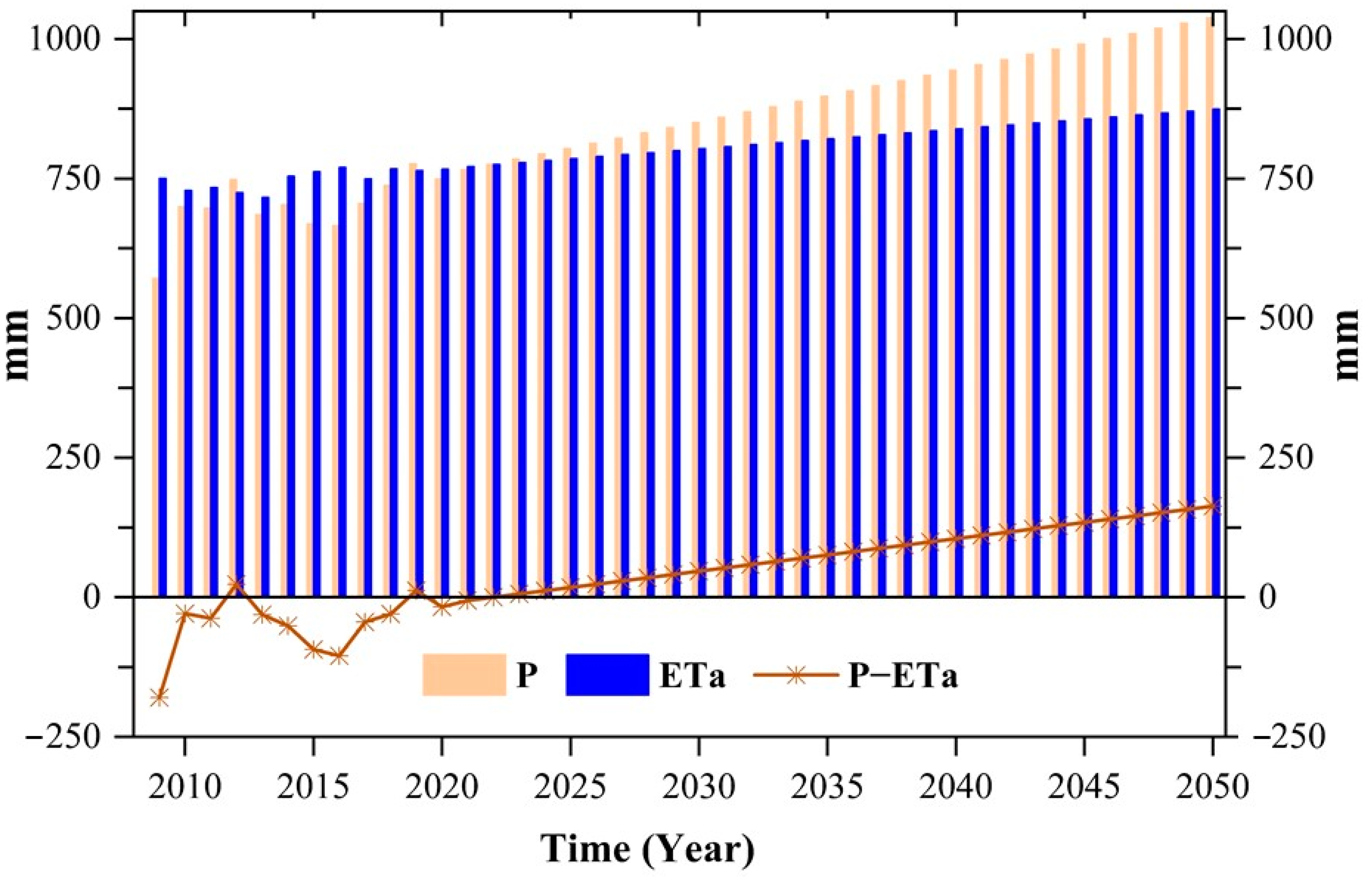
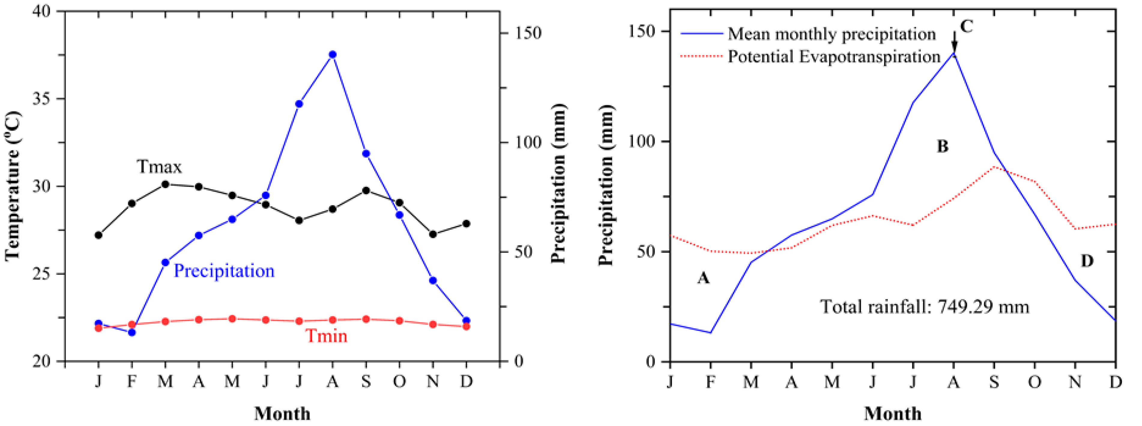
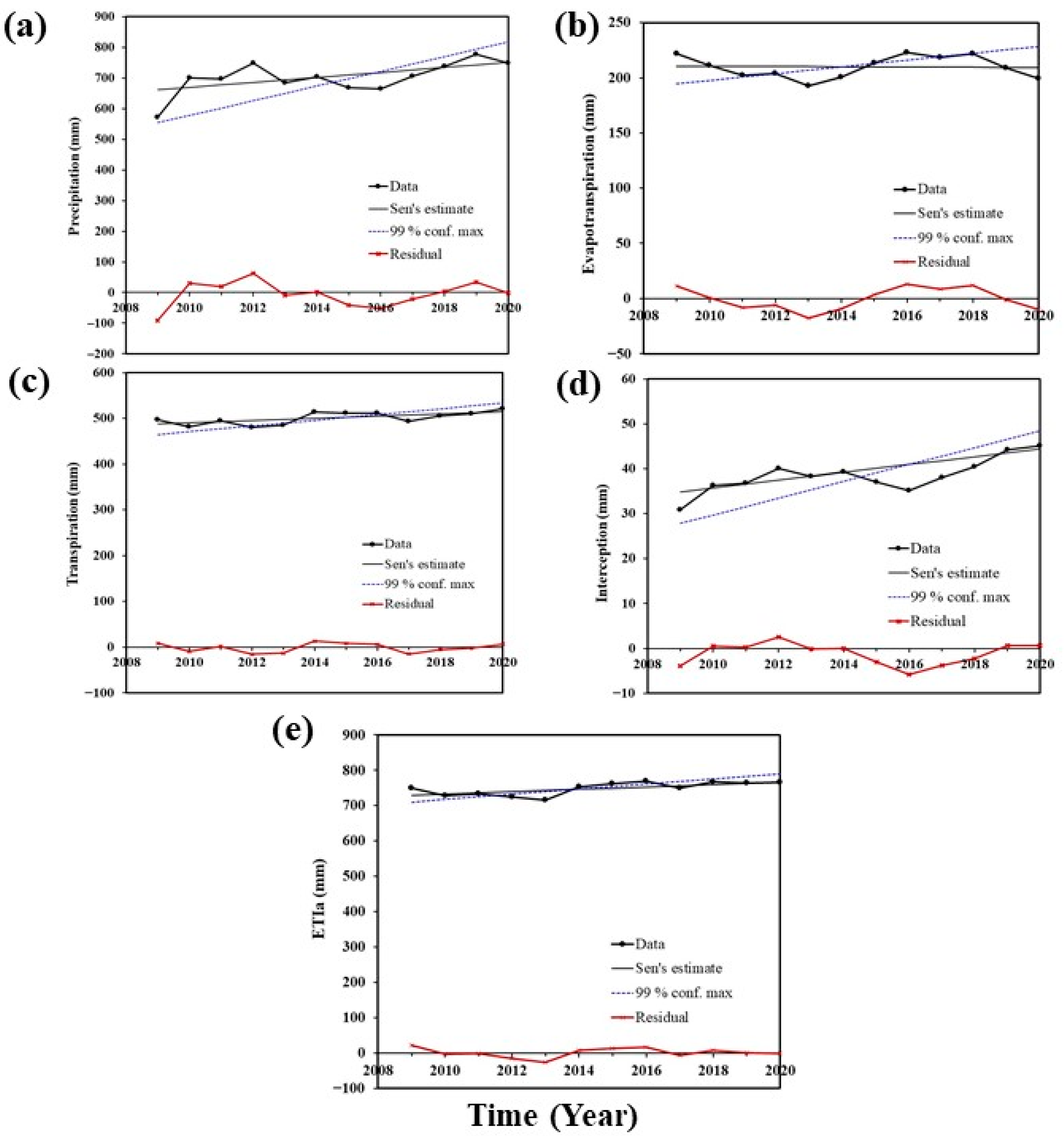
3.1. Long-Term Temporal Variability and Trends in Climatic Factors in the NRB

The preliminary analysis for this study included computing the mean and cumulative values in the annual precipitation (P), evapotranspiration (ET), transpiration (T), evaporation (E) interception (I), and ETIa time series for the whole NRB basin (

Table 3. Sen’s slope, Z statistics of Mann–Kendall (MK) trends for annual P, ET, T, E during 2009–2020 over NRB.

			MK Test		Sen’s Slope Estimate
Parameters	Time Series	n	Test Z	Significant Trends	Q	B
P	2009–2020	12	1.85	+	8.117	661.23
ET	2009–2020	12	−2.81	**	−11.030	2518.06
T	2009–2020	12	1.71	+	2.424	488.60
E	2009–2020	12	−0.07		−0.111	210.63
I	2009–2020	12	2.54	*	0.872	34.84
ETIa	2009–2020	12	1.99	*	3.473	728.87

Note: ** statistically high significant trend, * significant trend, and + non-significant trend at 95% confidence level, respectively.

). The results showed a mix of positive and negative trends for various hydro-climatic variables. The mean annual P varied between 570.86 mm and 776.36 mm while the mean annual ET varied between 2350.38 mm and 2542.2 mm in the basin. As reflected in Table 3, the data were not normally distributed. In the NRB, a significant monotonically increasing trend (8.117 mm·year⁻¹) of precipitation was detected in the study period (2009–2020). On the contrary, a strong positive correlation between P and time was observed by a relatively low MK Test Z value (1.85) for P, i.e., rainfall increased considerably as the year progressed from 2009 to present. However, the insignificance may be due to the different time span from the present study.

The interannual variability and annual mean trends of hydro-climatic variables during the 2009–2020 study period across the NRB are represented in Figure 5. Sen’s slope estimator curve was used to determine the trend magnitude, which was estimated by computing the least-squares estimate using linear regression. In 2009, the ETo, P, and T were 2541.96 mm, 776.36 mm, and 514.07 mm, respectively. Overall, the curve based on the time series data suggested a decline in precipitation and an increase in evapotranspiration. Besides, while the trend in Figure 5 varies slightly every year, but the overall trend has remained the same.

3.2. Estimation of Water Balance (WB) and Climatic Water Deficit (CWD) within the NRB

The P, ETa, and I were used to identify the areas and periods of the basin that generated water and the areas that consumed water. The periods where P was more than ETa and I were considered as water generating areas and those P less than ETa and I were considered as net consumers. To assess the WB in the basin for 2009 to 2020 and project from 2020 to 2050, we simply used the climatology method at the basin level. We compared the P, ETa, and P − ETa values (Figure 6). The changes in P − ETa indicated that the P − ETa is negative except for the years 2012 (23.45 mm or ~71.2 km³) and 2019 (12.23 mm or ~37.05 km³), which were the only years in the decade from 2009 when precipitation was more than evapotranspiration. The P − ETa was expected to rise to 163.34 mm or ~494.57 km³ by 2050 (Figure 6). This indicated that more water was being consumed than generated in the basin by abstracting from the storage in the basin. P − ETa is thus the variable that combines the model performance in temperature and precipitation and reflects the difference between precipitation (P) and actual evapotranspiration (ETa). P − ETa is important from a hydroclimatic perspective because it is a measure of water stress or deficit. Therefore, the consistent negative change in P − ETa indicates an overall increased water stress over the region.

Figure 7 depicts monthly variations in precipitation and PET across the NRB. The wet season is defined by excess precipitation over evapotranspiration (i.e., moisture surplus), whereas the dry season is characterized by the condition of excess evapotranspiration over precipitation (i.e., water deficit). The NRB has a high diversity in climate with greatly varied precipitation. In addition, the climate in the NRB is characterized by long summer growing seasons. During the summer, the average temperature is around 30 °C, with winter temperatures ranging between 5 and 10 °C. The majority of the basin experiences a single rainy season in the summer. There is a single rain peak in the Eastern Nile and Main Nile sub-basins, from June to October, with little or no rainfall in the other months. On one hand, in northern Uganda and South Sudan, as in Juba, rainfall is fairly uniformly distributed, with a single peak from April to October. The southern part of the NRB, on the other hand, experiences a twin peak distribution with high rainfall during March through May and September through November. Climate normals of the NRB between 2009 and 2020 reflect temperatures ranging from 30.1 to 15.1 °C in March and January, respectively. The highest mean annual precipitation is 140 mm. The Thornthwaite-type water balance models show high levels of annual CWD, which have increased at almost one from 2009 to 2020 (Figure 7).

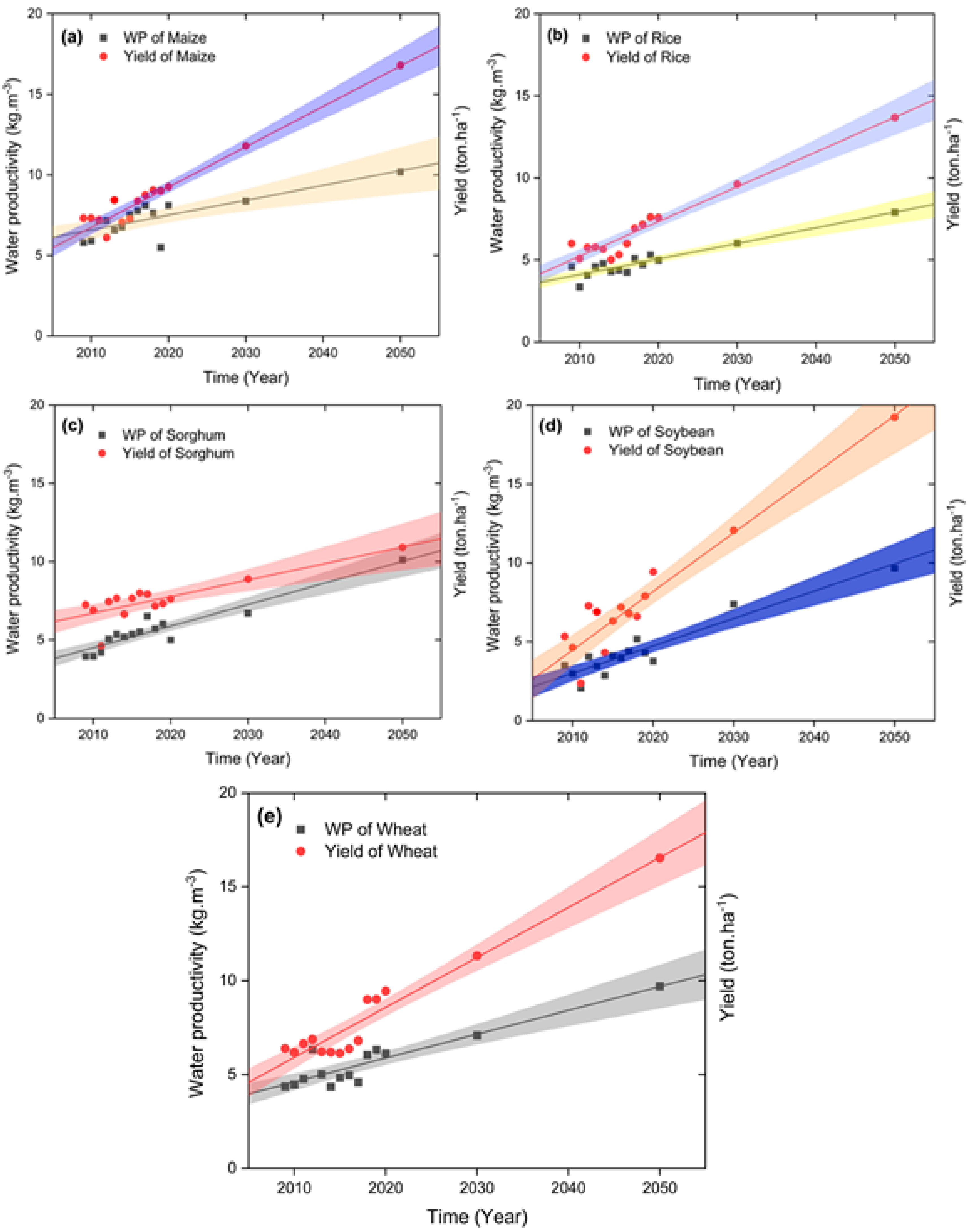
3.3. Seasonal Water Productivity and Yield of Major Crops

The expected annual and cumulative CWP and crop yield for major crops (i.e., maize, rice, sorghum, soybean, and wheat) based on seasonal variations are shown in Figure 8. The CWP and yield of major crops are highly correlated. In 2020, wheat had a higher yield (9.45 ton·ha⁻¹) compared to soybean (9.43 ton·ha⁻¹), maize (9.26 ton·ha⁻¹), rice (7.58 ton·ha⁻¹), and sorghum (7.61 ton·ha⁻¹). The mean CWP of maize is also higher (8.10 kg·m⁻³) compared to wheat (6.13 kg·m⁻³), rice (5.00 kg·m⁻³), sorghum (5.00 kg·m⁻³), and soybean (3.75 kg·m⁻³). In addition, the annual yield of soybean, maize, sorghum, wheat, and rice is expected to reach 19.24 ton·ha⁻¹, 16.8 ton·ha⁻¹, 16.8 ton·ha⁻¹, 16.53 ton·ha⁻¹, and 13.69 ton·ha⁻¹, respectively, by 2050. The WP of maize, sorghum, wheat, soybean, and rice is expected to reach 10.18 kg·m⁻³, 10.18 kg·m⁻³, and 9.7 kg·m⁻³, 9.66 kg·m⁻³, respectively, by 2050. The CWP as the crop yield to the crop water use is increasing in time and scale in the NRB due to agricultural activities and climatic factors such as high temperature, solar radiation, and precipitation. It should be noted that the species and varieties of crops greatly affect water use and crop yield.

3.4. Correlation between Water Use Efficiency (WUE) and Crop Water Productivity (CWP) for Major Crops

The results of the seasonal correlation coefficient (R) analysis of major crops are presented in Figure 9. Both negative and positive relationships exist among the variables. The largest changes in R are generally associated with large changes in WUE and CWP. As can be seen in Figure 9, the sorghum and wheat showed relatively smaller correlations with WUE while the rice, soybean, and maize showed relatively greater correlations. The variables of CWP of major crops are strongly positively correlated. It should be noted that the correlation coefficients along the diagonal of the graph are equal to 1 because each variable is perfectly correlated with itself. The correlation variables of CWP for soybean, sorghum, rice, wheat, and maize are 1, 0.70, 0.59, 0.55, and 0.31, respectively, (Figure 9a), while WUE for soybean, maize, sorghum, rice, and wheat are 1, 0.41, −0.51, 0.45, and −0.02, respectively (Figure 9b). Howbeit, WUE and CWP displayed quite similar patterns. The average values ET and crop yield for CWP and WUE in the NRB countries are shown in

Table 4. Average yield and ET values for CWP and WUE in the NRB countries for 2009–2020.

2009–2020
	Wheat				Rice				Sorghum				Maize				Soybean
Country	ET	Y	CWP	WUE	ET	Y	CWP	WUE	ET	Y	CWP	WUE	ET	Y	CWP	WUE	ET	Y	CWP	WUE
	mm	ton·ha−1	kg·m−3	kg·m−3	mm	ton·ha−1	kg·m−3	kg·m−3	mm	ton· ha−1	kg·m−3	kg·m−3	mm	ton·ha−1	kg·m−3	kg·m−3	mm	ton·ha−1	kg·m−3	kg·m−3
BUR	430.20	9.81	8.18	2.91	105.7	6.4	8.22	1.8	343.5	8.1	5.77	2.01	320	8.4	6.96	1.82		6.1	6.5	2.70
DRC	521.2	8.9	6.5	2.09	597.9	6.63	4.31	1.2	737.7	4.8	3.5	2.39	428.2	4.4	2.74	3.81	1279.1	7.76	6.3	2.27
EGY	508.2	6.72	6.5	2.09	774.4	8.67	4.85	1.21	691.9	7.8	8.4	1.84	571.1	7.9	5.9	1.82	1083	3.01	1.85	0.47
ERT	1480.4	1.69	1.67	0.10	1550	0.29	3.40	0.05	1414.1	2.3	3.22	0.81	1068.9	1.5	3.31	0.42	1480.4	0.81	1.78	0.47
ETH	687.8	2.5	4.92	1.31	597.9	3.17	4.31	1.2	343.5	4.47	5.77	2.01	428.2	3.00	12.74	3.81	1068	2.4	1.85	0.47
KEN	796.5	11.03	4.16	1.36	743	7.21	4.8	1.21	974.3	11.9	4.1	1.67	753.6	5.1	3.45	1.07	296.8	3.9	6.36	2.27
RWA	518.8	6.52	6.76	1.70	670	8.09	7.41	1.44	694	10.08	7.51	2.3	493.1	9.4	6.8	2.13	345.2	6.01	7.31	1.88
SSD	1779.8	1.69	1.6	0.1	756.3	0.29	3.4	0.05	1141.1	2.3	3.22	0.8	1141.1	1.5	3.31	0.42	1068.9	0.81	1.78	0.47
SUD	521.2	6.5	6.5	2.09	0	5.12	2.1	0.5	1068.9	1.7	3.4	0.44	1190.5	3.7	5.3	1.0	1430.9	1.85	2.4	0.47
UGA	712.2	11.10	5.65	1.82	449.1	5.72	5.45	1.56	566.2	11.8	7.32	2.3	428.2	14.4	12.74	3.81	359.8	5.69	5.25	1.76
TZN	687.8	6.00	4.92	1.31	795.5	10.2	4.3	1.59	694	10.9	6.59	1.84	707.9	12.8	6.03	2.40	743.9	8.85	3.4	1.07

Note: BUR: Burundi, DRC: Democratic Republic of Congo, EGY: Egypt, ERT: Eritrea, ETH: Ethiopia, KEN: Kenya, RWA: Rwanda, SSD: South Sudan, SUD: Sudan, UGA: Uganda, TZN: Tanzania.

.

3.5. Water Accounting and Saving Potential Analysis

The first step in water accounting was to define the spatiotemporal water accounting domain. The accounts were performed on an annual time step covering the years 2009 and 2020. To obtain areal values of WA, the yearly changes in P, ETa, ET_rain, and ET_incr were assessed (Figure 10). The results indicated that ET_rain followed the same trend as P except for the year 2012, which was in the wet year in the studied period. ET_incr showed an opposite trend with the precipitation. ET_incr decreased when precipitation increased and increased as P decreased. This indicated that part of the ET_incr was supplied from the groundwater sources or uncertainty was associated with WaPOR P and ETa. This also explained the fact that ET was greater than precipitation in almost all the years except for the wet year of 2012 and 2019. However, since reliable sources of groundwater abstraction were not found, any consumption from the groundwater was not included in the water accounts study.

Amidst the study period of 2009–2020, the year of 2012 received 2265.13 km³, or 748 mm, of rainfall. The exploitable water resources were 154.4 km³·year⁻¹, which was very different from that of the average situation. The main difference was in the amount of water stored in the basin, which now increased to 71.7 km³·year⁻¹. The proportion of ET_rain and ET_incr more or less remained the same. On the other hand, the year of 2016 was the driest year and received just 1981.9 km³·year⁻¹, or 633 mm·year⁻¹, less than the consumed water (i.e., 180.3 km³·year or the difference of supplied from depleting the storage in the basin). ET_incr (i.e., 185.1 km³·year⁻¹) was now 9% of the total consumed water. Besides, ET_incr showed a reduction of 13.4 km³·year⁻¹, with part of it satisfied by rainfall. The total consumption was 65.3 km³·year⁻¹, which accounted for 79% of the precipitation the basin received. ET_incr was only 20% of the total consumption. Moreover, the average water consumption (i.e., the sum of rainfall and increment ET) was 2163.8 km³·year⁻¹, which was higher than the precipitation. This resulted in utilized land use with the net inflow equal to 2202 km³·year⁻¹ (Figure 11). The majority of the available water resources went to utilized land use such as agricultural activities. Rarely, the usage of blue water (i.e., precipitation) appeared in water allocation plans since this consumption occurred naturally and was out of sight from water managers.

The main water-saving potentials in NRB are shown in Figure 10. The $\mathsf{\Delta }\mathrm{S}$indicates the change in total water storage (S). The Net Inflow (NIF) represents the gross inflow (GIF) and the storage (S). Gross inflow (GIF) refers to total inflow from all sources. Exploitable water (EW) indicates the net inflow minus Landscape ET (ET_land). Non-consumed water/outflow (OF) indicates the total outflow. Consumed water or ET indicates the total evapotranspiration (i.e., evapotranspiration from non-manageable, manageable, and managed land uses). ET_land occurs naturally, not due to water management (i.e., evaporation of managed reservoir or ET from irrigation water), whereas ET occurs as interception, evaporation, soil evaporation, water evaporation, or canopy transpiration. Increment ET (ET_incr) describes the ET that occurs from other sources except effective rainfall and interception. Rainfall ET (ET_rain) represents the ET that occurs from effective rainfall and canopy.

4. Discussion

4.1. Variability and Trends in Hydro-Meteorological Factors

In this study, we used the state-of-the-art process-based WaPOR dataset to analyze long-term spatiotemporal variations and related components in the NRB under hydroclimatic conditions. Figure 5 illustrates the variation of hydrometeorological indicators in the region on the area basis. The hydroclimatic factors indicated a mixture of positive and negative correlations for different variables (Table 3). The results of this study were consistent with the findings of numerous previous studies. Many studies have evaluated the trends in precipitation (P), evapotranspiration (ET), transpiration (T), evaporation (E), interception (I), and ETIa time series in NRB using the MK test and Sen’s slope estimator. Generally, the findings of related studies matched with the results obtained for this assessment. For instance, on the prior study [80] reported a significant increase and decrease in rainfall in different regions of the NRB. In another study, significant decreasing trends of −40.3 and −168.1 mm·year⁻¹ per decade in annual precipitation were observed in the upper Nile River Basin [81]. Alemu et al. [82] found that 65% of the study area (2.5 million km²) showed significant (p-value < 0.05) positive correlations between monthly ET and rainfall, whereas 7% showed significant negative correlations. The MK test results (Table 3) indicated that the test Z statistics of ET were generally consistent with those calculated by Samy et al. [83]. ET, one of the major components of water balance over the NRB, accounts for about 87% of the basins rainfall but varies from one sub-basin to another with time, depending on the type of LUC and the prevailing climatic conditions.

4.2. Water Balance and Climate Water Deficit

Interannual variability analysis revealed that the magnitude and temporal variation were reasonable and consistent with mean annual P over the region [82,84] which was in agreement with the findings of this study. ET and its components in the NRB followed a distinct seasonal cycle, with ET peaking in wet seasons and minima occurring in dry seasons [85]. The ET peak in September, falling to the minimum in winter (February), explained the distinct ET climatology of the region and indicated how different vegetation species assimilated available energy and water across the various climatic regions [86]. Our analysis (Figure 7) showed that the ET varied from 50.21 to 88.4 mm·year⁻¹ for the year of 2020. This variation trend was due to interannual P variability and agreed with previous studies in the basin [87,88]. Nooni et al. [89] revealed that areas with a slight increase in ET trends were mainly located in arid regions and some parts of semi-arid regions. This might be the reason for CWD in the basin. Using a regional model under RCP4.5 and RCP8.5 climate scenarios of four General Circulation Models (GCMs) of CMIP5 over NRB for the 2050s, the investigation on climate change impact on the future P and temperature indicated an increase by about 1.67–2 °C in five sub-basins. As this study employed the WaPOR, it was observed that the P and ETa had inherent errors, especially for low values. Thus, the water balance may not be very accurate.

4.3. Situation of CWP and WUE under the Crop Yield

This study used the AquaCrop model to simulate daily biomass production and final crop yield in response to water supply and consumption and agronomic management [69]. The model requires several parameters and input data to simulate yield in response to water for most of the major field crops cultivated worldwide [90]. Here, we considered only the rainfed agriculture in the basin.

Crop water use (CWU) is the average simulated evapotranspiration (ET) of major crops under rainfed conditions from sowing to maturity. The average CWU, multiple crop cycles per year, is feasible in a given location. The results based on annual calculations in the period of 2009–2020 [91,92,93] showed that the average simulated yield for major cereals was 6.3 ton·ha⁻¹ in East Africa, which was in agreement with our results (Figure 8). The average yield trends of wheat, maize, and rice were equivalent to about 3.79 tons·ha⁻¹, 6.75 ton·ha⁻¹, and 11.5 ton·ha⁻¹, while CWP varied from 0.6–1.7 kg·m⁻³, 0.6–1.60 kg·m⁻³, and 1.12–2.70 kg·m⁻³ [93]. Besides, the result indicated that the grain yield of maize increased from 2.5 tons·ha^–1 under poor soil fertility conditions to 6.4 and 9.2 tons·ha^–1 of under near-optimal and non-limiting soil fertility conditions [94]. The high CWP also corresponded to the application of various agrichemicals (i.e., manure and chemical fertilizers) and agronomic activities management (i.e., mulching and irrigation). So far, these have led to high production, lower ET, reduced soil evapotranspiration, and improved soil water [95,96].

Over the last two decades, the mean WP of wheat grains was 0.96 to 1.11 kg·m⁻³ as a result of supplement irrigation, which was quite different from our results of 6.13 kg·m⁻³. Supplemental irrigation on its own was insufficient to support crop production. However, when combined with rainfall, it led to an increase in CWP in most years, particularly in the drier years. The study also showed that when rainfall was ignored and only irrigation water was considered, CWP estimates were significantly higher. The combination of rainfall and irrigation water was documented in Kenya, where supplemental irrigation was applied to rainfed crops [97].

4.4. Water Accountings and Savings Potentialities

The findings presented in Figure 11 gave us an overview of current water resources and their potentialities in the study area. It also indicated that the main water accounting must be taken into consideration while exploiting the basin. The terrestrial water storage of NRB included groundwater, soil moisture, surface water bodies (lakes, rivers, and reservoirs), and canopy water storage. However, The NRB is based on two main sources of water: the first source is Lake Tana (85%), located in the east of the middle region, and the second source is Lake Victoria (15%), lying in the southern region [98]. Results of recent research that utilized GRACE-TWS data to study the changes in key water storage and hydrological mass variation in the basin were in agreement with the findings of this study [99]. From 2009 to 2020, the water storage was about 80 km³, which was in line with the study of [100]. Basin-wide annual water storage showed an interannual variability of up to 9% (±180 km³) of the total volume of basin precipitation (~2048 km³) for the period of 2002−2013. The natural land covers contribute the largest portion of water consumed in the basin. The water saved from water conservation can be used to reclaim a large portion of hyper and semi-arid areas for agricultural purposes, thus solving the food shortage problem.

4.5. Limitations of the Study

Although this research was extensive, it had some potential limitations. The current study assessed the agro-hydro-meteorological factors using the MK trend test [101], which basically involved a large and continuous dataset. So, it provided limited insight into the trend’s causative factor(s). Similarly, the study of Adeboye et al. [102] reported that the AquaCrop model overestimated the yield (Y) of major cereal grains (e.g., maize and soybean) at 25 and 50%. This may be described as one of the weaknesses of the model. As this research was not based on field assessments of CWP and WUE, socioeconomic indicators were not taken into consideration. The secondary data revealed some errors from one dataset to another. Due to insufficient of Ecosystem Research Networks (ERNs), updated and high-quality data were not available in Burundi, Democratic Republic of Congo (DRC), Sudan, and South Sudan. Nonetheless, the averaged values were used since they made a fair sense about the central tendency of the vast study area. Furthermore, this study identified all uncertainties in measurement accuracy that may have occurred during the analysis and in the results.

4.6. Policy Implications and Future Directions

The assessment of CWP and WUE situation provided a clear insight on water account potentials in NRB. Evaluating water accountings and potentialities will help water managers and policy-makers define goals that can greatly increase the crop yield from the sub-basin to the basin level. Based on the overall findings, the CWP was found to be mainly controlled by climate factors, plant-specific factors, and crop management practices [93]. To achieve sustainable CWP and WUE, there is a need to take full advantage of all available resources and their interconnections. For instance, reducing evaporation from water applied to irrigated fields through capital intensive and innovative technologies (e.g., drip irrigation) by considering the climatic, edaphic, and other factors or better agronomic practices (i.e., mulching or changing crop planting dates to match periods of less evaporative demand) or conservation agriculture (e.g., land leveling or zero tillage) should be promoted. Furthermore, in absentia of advanced agrarian technology, rain-fed agriculture could potentially help the development of sustainable agriculture in the NRB countries. Hitherto, despite these assertions, their practicability needs to be evaluated to avoid impacts on climate change, water scarcity, and rising demands, which can be achieved by the so-called food-energy-water-biodiversity-human health (WEFBH) nexus planning [8].

The extension of water-specific modern observation models, networks, and evaluations of new remote sensing technologies is the key to successful water resource management [103]. Remote sensing data have been utilized to provide information in data-scarce regions to account for foundational dynamic ecosystem shifts and climate variability [104]. Perfectly, the relationship among model parameters (e.g., AquaCrop model) and the phenomena that are being simulated can be iteratively compatible to avoid constraining model-data uncertainties and interpretation failures.

Yet the lack of transboundary cooperation, common methodologies, insufficient ecosystem research networks (i.e., data sharing), and several conflicts hinder the development of any riparian regions [105]. However, cooperation between transboundary basins is a fundamental requirement for implementing the basin approach and the principles of integrated water resources management.

5. Conclusions

The CWP and WA procedures are regarded as the ‘‘silver bullets’’ for analyzing water use and consumption in terms of water balance at the basin level. The NRB in EA confronts solemn water management challenges to keep alive vibrant agriculture due to a coupled semi-arid environment, water-intensive crops, and limited water supply. Accurate and reliable WP and WA information is required to assess and improve the current water management strategies. This research assessed the CWP and WA during 2009–2020. The Mann–Kendall (MK) test was conducted, and Sen’s slope estimate was used to evaluate the trend of the hydrometeorological time series. The AquaCrop model simulations for major crops in different periods revealed that the CWP and WUE in NRB were influenced by hydrometeorological factors and changed over time and space. Over the basin, an assessment of the inter-annual variability and trends showed the mean annual P varied between 570.86 mm and 776.36 mm while the mean annual ET varied between 2350.38 mm and 2542.2 mm in the basin. The ETa had the largest contribution in the first stage. Moreover, it was found that during May to June, a drier period separated the rainy and small rainy seasons until August, when rainfall attained its maximum amount (749.29 mm). This was true except for the years of 2012 (71.3 km³) and 2019 (37.05 km³), which were the years in the decade since 2009 where precipitation was more than ET. The CWD was expected to rise to ~494.57 km³ by 2050 due to high water abstraction from the storage, which would result in water deficit or stress. Therefore, the CWP and yield of major crops are highly correlated. Sorghum and wheat showed relatively smaller correlations with WUE while the rice, soybean, and maize showed relatively greater correlations. The findings revealed that ET_rain followed the same changes as P except for the year 2012, which was in the wet year in the studied period. The main difference was in the amount of water stored in the basin, which now increased to 71.7 km³·year⁻¹. Thus, NRB motivation policies for maximizing CWP and WUE should be considered carefully to conserve the water resource of the study area. The study also highlighted WP as a means to establish the most appropriate production systems. WP should serve as a goal to bring together various stakeholders. CWP, WUE, and crop production should be improved by promoting water-saving irrigation technology, enhancing the use of fertilizers, agricultural film, and agricultural pesticides, and improving the use efficiencies of agronomic inputs without increasing the amount. This study provides the basis for exploring ways of improving CWP and WUE, and more specific schemes still need to be developed. Finally, the transboundary water cooperation mechanism would be a very promising commitment.

References

1. Kummu, M.; Guillaume, J.H.A.; de Moel, H.; Eisner, S.; Flörke, M.; Porkka, M.; Siebert, S.; Veldkamp, T.I.E.; Ward, P.J. The world’s road to water scarcity: Shortage and stress in the 20th century and pathways towards sustainability. Sci. Rep. 2016, 6, 38495. [Google Scholar] [CrossRef] [PubMed] [Green Version]
2. Boretti, A.; Rosa, L. Reassessing the projections of the World Water Development Report. NPJ Clean Water 2019, 2, 15. [Google Scholar] [CrossRef]
3. Mishra, B.K.; Kumar, P.; Saraswat, C.; Chakraborty, S.; Gautam, A. Water Security in a Changing Environment: Concept, Challenges and Solutions. Water 2021, 13, 490. [Google Scholar] [CrossRef]
4. Alsharhan, A.S.; Rizk, Z.E. Challenges Facing Water Resources. In Water Resources and Integrated Management of the United Arab Emirates; Springer International Publishing: Cham, Switzerland, 2020; pp. 501–529. [Google Scholar]
5. Oyebande, L. Water problems in Africa—How can the sciences help? Hydrol. Sci. J. 2001, 46, 947–962. [Google Scholar] [CrossRef] [Green Version]
6. Searchinger, T.; Waite, R.; Hanson, C.; Ranganathan, J.; Dumas, P.; Matthews, E.; Klirs, C. Creating a Sustainable Food Future: A Menu of Solutions to Feed Nearly 10 Billion People by 2050; Final Report; WRI: Washington, DC, USA, 2019. [Google Scholar]
7. UN. World Population Prospects: The 2015 Revision: Key Findings and Advance Table; United Nations: New York, NY, USA, 2015. [Google Scholar]
8. Hirwa, H.; Zhang, Q.; Qiao, Y.; Peng, Y.; Leng, P.; Tian, C.; Khasanov, S.; Li, F.; Kayiranga, A.; Muhirwa, F.; et al. Insights on Water and Climate Change in the Greater Horn of Africa: Connecting Virtual Water and Water-Energy-Food-Biodiversity-Health Nexus. Sustainability 2021, 13, 6483. [Google Scholar] [CrossRef]
9. Hunter, M.C.; Smith, R.G.; Schipanski, M.E.; Atwood, L.W.; Mortensen, D.A. Agriculture in 2050: Recalibrating Targets for Sustainable Intensification. BioScience 2017, 67, 386–391. [Google Scholar] [CrossRef] [Green Version]
10. Molden, D.; Oweis, T.; Steduto, P.; Bindraban, P.; Hanjra, M.A.; Kijne, J. Improving agricultural water productivity: Between optimism and caution. Agric. Water Manag. 2010, 97, 528–535. [Google Scholar] [CrossRef]
11. Kang, Y.; Khan, S.; Ma, X. Climate change impacts on crop yield, crop water productivity and food security—A review. Prog. Nat. Sci. 2009, 19, 1665–1674. [Google Scholar] [CrossRef]
12. Momblanch, A.; Papadimitriou, L.; Jain, S.K.; Kulkarni, A.; Ojha, C.S.P.; Adeloye, A.J.; Holman, I.P. Untangling the water-food-energy-environment nexus for global change adaptation in a complex Himalayan water resource system. Sci. Total Environ. 2019, 655, 35–47. [Google Scholar] [CrossRef]
13. Digna, R.F.; Mohamed, Y.A.; van der Zaag, P.; Uhlenbrook, S.; Corzo, G.A. Nile River Basin modelling for water resources management—A literature review. Int. J. River Basin Manag. 2017, 15, 39–52. [Google Scholar] [CrossRef]
14. UNEP-WCMC. Global Drylands: A UN System-Wide Response; United Nations Environment Management Group: Nairobi, Kenya, 2011. [Google Scholar]
15. Fadong, L.; Peifang, L.; Qiuying, Z.; Shuai, S.; Yunfeng, Q.; Congke, G.; Qian, Z.; Liang, W.; Balehegn, M.; Mojo, D.; et al. Understanding Agriculture Production and Food Security in Ethiopia from the Perspective of China. J. Resour. Ecol. 2018, 9, 237–249. [Google Scholar]
16. Siam, M.S.; Eltahir, E.A.B. Climate change enhances interannual variability of the Nile river flow. Nat. Clim. Chang. 2017, 7, 350–354. [Google Scholar] [CrossRef]
17. Bender, M.V. Water Management in East Africa. In Oxford Research Encyclopedia of African History; Oxford University Press: Oxford, UK, 2019. [Google Scholar]
18. Dirwai, T.L.; Kanda, E.K.; Senzanje, A.; Busari, T.I. Water resource management: IWRM strategies for improved water management. A systematic review of case studies of East, West and Southern Africa. PLoS ONE 2021, 16, e0236903. [Google Scholar] [CrossRef] [PubMed]
19. Wheeler, K.G.; Basheer, M.; Mekonnen, Z.T.; Eltoum, S.O.; Mersha, A.; Abdo, G.M.; Zagona, E.A.; Hall, J.W.; Dadson, S.J. Cooperative filling approaches for the grand Ethiopian renaissance dam. Water Int. 2016, 41, 611–634. [Google Scholar] [CrossRef]
20. Simonit, S.; Perrings, C. Sustainability and the value of the ‘regulating’ services: Wetlands and water quality in Lake Victoria. Ecol. Econ. 2011, 70, 1189–1199. [Google Scholar] [CrossRef]
21. Swallow, B.M.; Sang, J.K.; Nyabenge, M.; Bundotich, D.K.; Duraiappah, A.K.; Yatich, T.B. Tradeoffs, synergies and traps among ecosystem services in the Lake Victoria basin of East Africa. Environ. Sci. Policy 2009, 12, 504–519. [Google Scholar] [CrossRef]
22. Ruthenberg, H. Agricultural Development in Tanganyika; Springer: Berlin/Heidelberg, Germany, 2013; Volume 2. [Google Scholar]
23. Teshome, B.W. Transboundary Water Cooperation in Africa: The Case of the Nile Basin Initiative (NBI). Altern. Turk. J. Int. Relat. 2008, 7, 34–43. [Google Scholar]
24. Petrov, T.E. The Grand Ethiopian Renaissance Dam: Risk of Interstate Conflict on the Nile; Naval Postgraduate School: Monterey, CA, USA, 2018. [Google Scholar]
25. Ndunda, E. Kenya: States to Sign Nile Accord Next Month; Standard, AllAfrica: Washington, DC, USA, 2006; Available online: https://allafrica.com/stories/200611201862.html (accessed on 18 January 2022).
26. Ligate, F.; Ijumulana, J.; Ahmad, A.; Kimambo, V.; Irunde, R.; Mtamba, J.O.; Mtalo, F.; Bhattacharya, P. Groundwater resources in the East African Rift Valley: Understanding the geogenic contamination and water quality challenges in Tanzania. Sci. Afr. 2021, 13, e00831. [Google Scholar] [CrossRef]
27. Mellor, J.E.; Watkins, D.W.; Mihelcic, J.R. Rural water usage in East Africa: Does collection effort really impact basic access? Waterlines 2012, 31, 215–225. [Google Scholar] [CrossRef] [Green Version]
28. Hope, R.; Thomson, P.; Koehler, J.; Foster, T. Rethinking the economics of rural water in Africa. Oxf. Rev. Econ. Policy 2020, 36, 171–190. [Google Scholar] [CrossRef] [Green Version]
29. Thompson, J.; Porras, I.T.; Wood, E.; Tumwine, J.K.; Mujwahuzi, M.R.; Katui-Katua, M.; Johnstone, N. Waiting at the tap: Changes in urban water use in East Africa over three decades. Environ. Urban. 2000, 12, 37–52. [Google Scholar] [CrossRef]
30. Conway, D.; Allison, E.; Felstead, R.; Goulden, M. Rainfall variability in East Africa: Implications for natural resources management and livelihoods. Philos. Trans. R. Soc. A Math. Phys. Eng. Sci. 2005, 363, 49–54. [Google Scholar] [CrossRef] [PubMed]
31. Kimaro, J. A Review on Managing Agroecosystems for Improved Water Use Efficiency in the Face of Changing Climate in Tanzania. Adv. Meteorol. 2019, 2019, 9178136. [Google Scholar] [CrossRef] [Green Version]
32. Mo, F.; Wang, J.-Y.; Li, F.-M.; Nguluu, S.N.; Ren, H.-X.; Zhou, H.; Zhang, J.; Kariuki, C.W.; Gicheru, P.; Kavagi, L.; et al. Yield-phenology relations and water use efficiency of maize (Zea mays L.) in ridge-furrow mulching system in semiarid east African Plateau. Sci. Rep. 2017, 7, 3260. [Google Scholar] [CrossRef] [PubMed] [Green Version]
33. Hengsdijk, H.; Smit, A.A.M.F.R.; Conijn, J.G.; Rutgers, B.; Biemans, H. Agricultural Crop Potentials and Water Use in East Africa; Plant Research International, Business Unit Agrosystems Research: Wageningen, The Netherlands, 2014. [Google Scholar]
34. Chukalla, A.D.; Mul, M.L.; van der Zaag, P.; van Halsema, G.; Mubaya, E.; Muchanga, E.; den Besten, N.; Karimi, P. A Framework for Irrigation Performance Assessment Using WaPOR data: The case of a Sugarcane Estate in Mozambique. Hydrol. Earth Syst. Sci. Discuss. 2021, preprint. [Google Scholar] [CrossRef]
35. Jha, A.K.; Malla, R.; Sharma, M.; Panthi, J.; Lakhankar, T.; Krakauer, N.Y.; Pradhanang, S.M.; Dahal, P.; Shrestha, M.L. Impact of Irrigation Method on Water Use Efficiency and Productivity of Fodder Crops in Nepal. Climate 2016, 4, 4. [Google Scholar] [CrossRef] [Green Version]
36. Hong, N.B.; Yabe, M. Improvement in irrigation water use efficiency: A strategy for climate change adaptation and sustainable development of Vietnamese tea production. Environ. Dev. Sustain. 2017, 19, 1247–1263. [Google Scholar] [CrossRef]
37. Pawlak, K.; Kołodziejczak, M. The Role of Agriculture in Ensuring Food Security in Developing Countries: Considerations in the Context of the Problem of Sustainable Food Production. Sustainability 2020, 12, 5488. [Google Scholar] [CrossRef]
38. Eldardiry, H.; Hossain, F. Understanding reservoir operating rules in the transboundary nile river basin using macroscale hydrologic modeling with satellite measurements. J. Hydrometeorol. 2019, 20, 2253–2269. [Google Scholar] [CrossRef]
39. Akurut, M.; Willems, P.; Niwagaba, C.B. Potential Impacts of Climate Change on Precipitation over Lake Victoria, East Africa, in the 21st Century. Water 2014, 6, 2634–2659. [Google Scholar] [CrossRef] [Green Version]
40. Senay, G.B.; Velpuri, N.M.; Bohms, S.; Demissie, Y.; Gebremichael, M. Understanding the hydrologic sources and sinks in the Nile Basin using multisource climate and remote sensing data sets. Water Resour. Res. 2014, 50, 8625–8650. [Google Scholar] [CrossRef]
41. Ainsworth, R.; Cowx, I.G.; Funge-Smith, S. A Review of Major River Basins and Large Lakes Relevant to Inland Fisheries; FAO Fisheries and Aquaculture Circular, No. 1170; FAO: Rome, Italy, 2021. [Google Scholar] [CrossRef]
42. Barnes, J. The future of the Nile: Climate change, land use, infrastructure management, and treaty negotiations in a transboundary river basin. WIREs Clim. Chang. 2017, 8, e449. [Google Scholar] [CrossRef]
43. Verdin, K. Hydrologic Derivatives for Modeling and Applications (HDMA) Database: US Geological Survey Data Release; US Geological Survey: Reston, VA, USA, 2017. [CrossRef]
44. Awulachew, S.B. The Nile River Basin: Water, Agriculture, Governance and Livelihoods; Routledge: London, UK, 2012. [Google Scholar]
45. Bouraoui, F.; Grizzetti, B.; Aloe, A. Estimation of water fluxes into the Mediterranean Sea. J. Geophys. Res. Atmos. 2010, 115, 1–12. [Google Scholar] [CrossRef]
46. Tate, E.L.; Sene, K.J.; Sutcliffe, J.V. A water balance study of the upper White Nile basin flows in the late nineteenth century. Hydrol. Sci. J. 2001, 46, 301–318. [Google Scholar] [CrossRef] [Green Version]
47. Dile, Y.T.; Tekleab, S.; Ayana, E.K.; Gebrehiwot, S.G.; Worqlul, A.W.; Bayabil, H.K.; Yimam, Y.T.; Tilahun, S.A.; Daggupati, P.; Karlberg, L. Advances in water resources research in the Upper Blue Nile basin and the way forward: A review. J. Hydrol. 2018, 560, 407–423. [Google Scholar] [CrossRef]
48. Coffel, E.D.; Keith, B.; Lesk, C.; Horton, R.M.; Bower, E.; Lee, J.; Mankin, J.S. Future Hot and Dry Years Worsen Nile Basin Water Scarcity Despite Projected Precipitation Increases. Earth’s Future 2019, 7, 967–977. [Google Scholar] [CrossRef] [Green Version]
49. Camberlin, P. Climate of Eastern Africa. In Oxford Research Encyclopedia of Climate Science; Oxford University Press: Oxford, UK, 2018. [Google Scholar] [CrossRef]
50. MacDonald, A.; Calow, R. Developing groundwater for secure rural water supplies in Africa. Desalination 2009, 248, 546–556. [Google Scholar] [CrossRef] [Green Version]
51. Powell, O.; Fensham, R. The history and fate of the Nubian Sandstone Aquifer springs in the oasis depressions of the Western Desert, Egypt. Hydrogeol. J. 2016, 24, 395–406. [Google Scholar] [CrossRef]
52. Bravard, J.-P.; Mostafa, A.; Garcier, R.; Tallet, G.; Ballet, P.; Chevalier, Y.; Tronchère, H. Rise and Fall of an Egyptian Oasis: Artesian Flow, Irrigation Soils, and Historical Agricultural Development in El-Deir, Kharga Depression, Western Desert of Egypt. Geoarchaeology 2016, 31, 467–486. [Google Scholar] [CrossRef]
53. Mancosu, N.; Snyder, R.L.; Kyriakakis, G.; Spano, D. Water Scarcity and Future Challenges for Food Production. Water 2015, 7, 975–992. [Google Scholar] [CrossRef]
54. Bucknall, J. Making the Most of Scarcity: Accountability for Better Water Management Results in the Middle East and North Africa; MENA Development Report; World Bank: Washington, DC, USA, 2007. [Google Scholar] [CrossRef]
55. FAO. WaPOR Database Methodology: Version 2 Release, April 2020; FAO: Rome, Itay, 2020. [Google Scholar] [CrossRef]
56. FAO. WaPOR, FAO’s Portal to Monitor Water Productivity through Open Access of Remotely Sensed Derived Data; FAO: Rome, Italy, 2020. [Google Scholar]
57. FAO. WaPOR V2 Quality Assessment–Technical Report on the Data Quality of the WaPOR FAO Database Version 2; Food and Agriculture Organization of the United Nations: Rome, Italy, 2020; p. 89. [Google Scholar]
58. Blatchford, M.; Mannaerts, C.M.; Zeng, Y.; Nouri, H.; Karimi, P. Influence of Spatial Resolution on Remote Sensing-Based Irrigation Performance Assessment Using WaPOR Data. Remote Sens. 2020, 12, 2949. [Google Scholar] [CrossRef]
59. NBI. Nile Basin: Water Resources Atlas; Nile Basin Initiative Secretariat (Nile-SEC): Entebbe, Uganda, 2017. [Google Scholar]
60. Dinku, T.; Funk, C.; Peterson, P.; Maidment, R.; Tadesse, T.; Gadain, H.; Ceccato, P. Validation of the CHIRPS satellite rainfall estimates over eastern Africa. Q. J. R. Meteorol. Soc. 2018, 144, 292–312. [Google Scholar] [CrossRef] [Green Version]
61. Li, B.; Rodell, M.; Kumar, S.; Beaudoing, H.K.; Getirana, A.; Zaitchik, B.F.; de Goncalves, L.G.; Cossetin, C.; Bhanja, S.; Mukherjee, A.; et al. Global GRACE Data Assimilation for Groundwater and Drought Monitoring: Advances and Challenges. Water Resour. Res. 2019, 55, 7564–7586. [Google Scholar] [CrossRef] [Green Version]
62. Biancamaria, S.; Mballo, M.; Le Moigne, P.; Sanchez-Perez, J.-M.; Espitalier-Noël, G.; Grusson, Y.; Cakir, R.; Häfliger, V.; Barathieu, F.; Trasmonte, M.; et al. Total water storage variability from GRACE mission and hydrological models for a 50,000 km2 temperate watershed: The Garonne River basin (France). J. Hydrol. Reg. Stud. 2019, 24, 100609. [Google Scholar] [CrossRef]
63. Di Gregorio, A. Land Cover Classification System: Classification Concepts. Software Version 3; FAO: Rome, Italy, 2016. [Google Scholar]
64. Ahlqvist, O. In search of classification that supports the dynamics of science: The FAO Land Cover Classification System and proposed modifications. Environ. Plan. B Plan. Des. 2008, 35, 169–186. [Google Scholar] [CrossRef] [Green Version]
65. Huntington, J.L.; Hegewisch, K.C.; Daudert, B.; Morton, C.G.; Abatzoglou, J.T.; McEvoy, D.J.; Erickson, T. Climate Engine: Cloud Computing and Visualization of Climate and Remote Sensing Data for Advanced Natural Resource Monitoring and Process Understanding. Bull. Am. Meteorol. Soc. 2017, 98, 2397–2410. [Google Scholar] [CrossRef]
66. Bastiaanssen, W.; Cheema, M.; Immerzeel, W.; Miltenburg, I.; Pelgrum, H. Surface energy balance and actual evapotranspiration of the transboundary Indus Basin estimated from satellite measurements and the ETLook model. Water Resour. Res. 2012, 48, W115112. [Google Scholar] [CrossRef] [Green Version]
67. Monteith, J.L. Evaporation and environment. In Symposia of the Society for Experimental Biology; Cambridge University Press (CUP): Cambridge, UK, 1965; Volume 19, pp. 205–234. [Google Scholar]
68. Foster, T.; Brozović, N.; Butler, A.; Neale, C.; Raes, D.; Steduto, P.; Fereres, E.; Hsiao, T.C. AquaCrop-OS: An open-source version of FAO’s crop water productivity model. Agric. Water Manag. 2017, 181, 18–22. [Google Scholar] [CrossRef]
69. Vanuytrecht, E.; Raes, D.; Steduto, P.; Hsiao, T.C.; Fereres, E.; Heng, L.K.; Garcia Vila, M.; Mejias Moreno, P. AquaCrop: FAO’s crop water productivity and yield response model. Environ. Model. Softw. 2014, 62, 351–360. [Google Scholar] [CrossRef]
70. Steduto, P.; Hsiao, T.C.; Fereres, E.; Raes, D. Crop Yield Response to Water; Food and Agriculture Organization of the United Nations: Rome, Italy, 2012; Volume 1028. [Google Scholar]
71. Mann, H.B. Nonparametric Tests against Trend. Econometrica 1945, 13, 245–259. [Google Scholar] [CrossRef]
72. Kendall, M.G. Rank Correlation Methods; Griffin: London, UK, 1948. [Google Scholar]
73. Ahn, K.-H.; Merwade, V. Quantifying the relative impact of climate and human activities on streamflow. J. Hydrol. 2014, 515, 257–266. [Google Scholar] [CrossRef]
74. Sen, P.K. Estimates of the regression coefficient based on Kendall’s tau. J. Am. Stat. Assoc. 1968, 63, 1379–1389. [Google Scholar] [CrossRef]
75. Lutz, J.A.; van Wagtendonk, J.W.; Franklin, J.F.; Williams, J. Climatic water deficit, tree species ranges, and climate change in Yosemite National Park. J. Biogeogr. 2010, 37, 936–950. [Google Scholar] [CrossRef]
76. Thapa, B.R.; Ishidaira, H.; Pandey, V.P.; Shakya, N.M. A multi-model approach for analyzing water balance dynamics in Kathmandu Valley, Nepal. J. Hydrol. Reg. Stud. 2017, 9, 149–162. [Google Scholar] [CrossRef]
77. Molden, D.; Sakthivadivel, R. Water accounting to assess use and productivity of water. Int. J. Water Resour. Dev. 1999, 15, 55–71. [Google Scholar] [CrossRef]
78. Batchelor, C.; Hoogeveen, J.; Faurès, J.-M.; Peiser, L. Water Accounting and Auditing: A Sourcebook; FAO Water Reports, No. 43; FAO: Rome, Itay, 2016. [Google Scholar]
79. Jägermeyr, J.; Gerten, D.; Heinke, J.; Schaphoff, S.; Kummu, M.; Lucht, W. Water savings potentials of irrigation systems: Global simulation of processes and linkages. Hydrol. Earth Syst. Sci. 2015, 19, 3073–3091. [Google Scholar] [CrossRef] [Green Version]
80. Onyutha, C. Statistical analyses of potential evapotranspiration changes over the period 1930–2012 in the Nile River riparian countries. Agric. For. Meteorol. 2016, 226–227, 80–95. [Google Scholar] [CrossRef]
81. Tabari, H.; Taye, M.T.; Willems, P. Statistical assessment of precipitation trends in the upper Blue Nile River basin. Stoch. Environ. Res. Risk Assess. 2015, 29, 1751–1761. [Google Scholar] [CrossRef]
82. Alemu, H.; Kaptué, A.T.; Senay, G.B.; Wimberly, M.C.; Henebry, G.M. Evapotranspiration in the Nile Basin: Identifying Dynamics and Drivers, 2002–2011. Water 2015, 7, 4914–4931. [Google Scholar] [CrossRef]
83. Samy, A.; Ibrahim, M.G.; Mahmod, W.E.; Fujii, M.; Eltawil, A.; Daoud, W. Statistical Assessment of Rainfall Characteristics in Upper Blue Nile Basin over the Period from 1953 to 2014. Water 2019, 11, 468. [Google Scholar] [CrossRef] [Green Version]
84. Mueller, B.; Seneviratne, S.I.; Jimenez, C.; Corti, T.; Hirschi, M.; Balsamo, G.; Ciais, P.; Dirmeyer, P.; Fisher, J.B.; Guo, Z.; et al. Evaluation of global observations-based evapotranspiration datasets and IPCC AR4 simulations. Geophys. Res. Lett. 2011, 38, L06402. [Google Scholar] [CrossRef] [Green Version]
85. Allam, M.M.; Jain Figueroa, A.; McLaughlin, D.B.; Eltahir, E.A. Estimation of evaporation over the upper b lue n ile basin by combining observations from satellites and river flow gauges. Water Resour. Res. 2016, 52, 644–659. [Google Scholar] [CrossRef] [Green Version]
86. Hasler, N.; Avissar, R. What controls evapotranspiration in the Amazon basin? J. Hydrometeorol. 2007, 8, 380–395. [Google Scholar] [CrossRef]
87. Marshall, M.; Funk, C.; Michaelsen, J. Examining evapotranspiration trends in Africa. Clim. Dyn. 2012, 38, 1849–1865. [Google Scholar] [CrossRef]
88. Hilhorst, B. Information Products for Nile Basin Water Resources Management. In Synthesis Report; FAO: Rome, Itay, 2011. [Google Scholar]
89. Nooni, I.K.; Wang, G.; Hagan, D.F.T.; Lu, J.; Ullah, W.; Li, S. Evapotranspiration and its Components in the Nile River Basin Based on Long-Term Satellite Assimilation Product. Water 2019, 11, 1400. [Google Scholar] [CrossRef] [Green Version]
90. Biazin, B.; Wondatir, S.; Tilahun, G.; Asaro, N.; Amede, T. Using AquaCrop as a Decision-Support Tool for Small-Scale Irrigation Systems Was Dictated by the Institutional and Market Incentives in Ethiopia. Front. Water 2021, 3, 664127. [Google Scholar] [CrossRef]
91. Ramankutty, N.; Evan, A.T.; Monfreda, C.; Foley, J.A. Farming the planet: 1. Geographic distribution of global agricultural lands in the year 2000. Glob. Biogeochem. Cycles 2008, 22. [Google Scholar] [CrossRef]
92. Monfreda, C.; Ramankutty, N.; Foley, J.A. Farming the planet: 2. Geographic distribution of crop areas, yields, physiological types, and net primary production in the year 2000. Glob. Biogeochem. Cycles 2008, 22, GB1003. [Google Scholar] [CrossRef]
93. Morita. Chapter 5-Past trends in water productivity at the global and regional scale. In Current Directions in Water Scarcity Research; Kumar, M.D., Ed.; Elsevier: Amsterdam, The Netherlands, 2021; Volume 3, pp. 99–118. [Google Scholar]
94. Erkossa, T.; Awulachew, S.B.; Aster, D. Soil fertility effect on water productivity of maize in the upper blue nile basin, Ethiopia. Agric. Sci. 2011, 2, 238. [Google Scholar] [CrossRef] [Green Version]
95. Qin, W.; Hu, C.; Oenema, O. Soil mulching significantly enhances yields and water and nitrogen use efficiencies of maize and wheat: A meta-analysis. Sci. Rep. 2015, 5, 16210. [Google Scholar] [CrossRef]
96. Silungwe, F.R.; Graef, F.; Bellingrath-Kimura, S.D.; Tumbo, S.D.; Kahimba, F.C.; Lana, M.A. Crop Upgrading Strategies and Modelling for Rainfed Cereals in a Semi-Arid Climate—A Review. Water 2018, 10, 356. [Google Scholar] [CrossRef] [Green Version]
97. Rockström, J.; Barron, J. Water productivity in rainfed systems: Overview of challenges and analysis of opportunities in water scarcity prone savannahs. Irrig. Sci. 2007, 25, 299–311. [Google Scholar] [CrossRef]
98. Abd-Elbaky, M.; Jin, S. Hydrological mass variations in the Nile River Basin from GRACE and hydrological models. Geod. Geodyn. 2019, 10, 430–438. [Google Scholar] [CrossRef]
99. Awange, J.L.; Forootan, E.; Kuhn, M.; Kusche, J.; Heck, B. Water storage changes and climate variability within the Nile Basin between 2002 and 2011. Adv. Water Resour. 2014, 73, 1–15. [Google Scholar] [CrossRef] [Green Version]
100. Shamsudduha, M.; Taylor, R.G.; Jones, D.; Longuevergne, L.; Owor, M.; Tindimugaya, C. Recent changes in terrestrial water storage in the Upper Nile Basin: An evaluation of commonly used gridded GRACE products. Hydrol. Earth Syst. Sci. 2017, 21, 4533–4549. [Google Scholar] [CrossRef] [Green Version]
101. Yue, S.; Pilon, P. A comparison of the power of the t test, Mann-Kendall and bootstrap tests for trend detection/Une comparaison de la puissance des tests t de Student, de Mann-Kendall et du bootstrap pour la détection de tendance. Hydrol. Sci. J. 2004, 49, 21–37. [Google Scholar] [CrossRef]
102. Adeboye, O.B.; Schultz, B.; Adeboye, A.P.; Adekalu, K.O.; Osunbitan, J.A. Application of the AquaCrop model in decision support for optimization of nitrogen fertilizer and water productivity of soybeans. Inf. Process. Agric. 2021, 8, 419–436. [Google Scholar] [CrossRef]
103. Woldai, T. The status of Earth Observation (EO) & Geo-Information Sciences in Africa–trends and challenges. Geo-Spat. Inf. Sci. 2020, 23, 107–123. [Google Scholar] [CrossRef]
104. Smith, W.K.; Dannenberg, M.P.; Yan, D.; Herrmann, S.; Barnes, M.L.; Barron-Gafford, G.A.; Biederman, J.A.; Ferrenberg, S.; Fox, A.M.; Hudson, A.; et al. Remote sensing of dryland ecosystem structure and function: Progress, challenges, and opportunities. Remote Sens. Environ. 2019, 233, 111401. [Google Scholar] [CrossRef]
105. Skoulikaris, C. Transboundary Cooperation through Water Related EU Directives’ Implementation Process. The Case of Shared Waters between Bulgaria and Greece. Water Resour. Manag. 2021, 35, 4977–4993. [Google Scholar] [CrossRef]
Figure 1. Location map of East Africa and NRB. The Digital Elevation Model (DEM) from the Hydrologic Derivatives for Modelling and Analysis (HDMA) database was used [43]. The map was developed using ArcGIS 10.6 (http://www.esri.com/software/arcgis/arcgis-for-desktop, accessed on 24 October 2021).
Agronomy 12 00818 g001
Figure 2. Land cover pattern in the NRB.
Agronomy 12 00818 g002
Figure 3. Simplified flowchart of the water accounting and water productivity methodology assessment to determine the saving potential.
Agronomy 12 00818 g003
Figure 4. Comparison between the daily precipitation (collected from CHIRPS dataset) and precipitation (collected from WaPOR) at Jinja, Gambela, Karima, and Aswan meteorological stations from 2009 to 2020. The red line indicates the linear fit between values.
Agronomy 12 00818 g004
Figure 5. Interannual variability in (a) precipitation, (b) evapotranspiration, (c) transpiration, (d) interception, and (e) ETIa from 2009 to 2020 across the NRB.
Agronomy 12 00818 g005
Figure 6. Comparison of yearly average variation of precipitation (P), ETa, and P − ETa in the NRB for the period 2009–2050.
Agronomy 12 00818 g006
Figure 7. Model of water budget in the NRB for the year 2020. A and D: Climatic Water Deficit (CWD): The potential evapotranspiration is greater than precipitation. The water store is being used up by plants of lost through evaporation (soil moisture utilization). As the store of water is depleted, and potential evapotranspiration exceeds precipitation, there is a deficiency of soil water. Crops must have adaptation behaviors and they must be irrigated. B: Water Surplus: Precipitation exceeds potential evapotranspiration. The soil water store is full and there is a soil moisture surplus for plant use, runoff, and groundwater recharge. C: Field capacity has been reached. Additional rainfall will percolate down to the water table, and groundwater stores will be recharged.
Agronomy 12 00818 g007
Figure 8. CWP and CY in NRB countries from 2009 to 2050. Cumulative of (a) Maize, (b) Rice, (c) Sorghum, (d) Soybean, and (e) Wheat based on higher, average, and lower levels.
Agronomy 12 00818 g008
Figure 9. Pearson’s correlation coefficients for the relationship between (a) CWP (kg·m−3) and (b) WUE (kg.m−3) for the five major crops in NRB during 2009–2020. The diameter of the sphere represents −1 (i.e., strong negative correlation), 0 (i.e., no relationship), and +1 (i.e., strong positive correlation).
Agronomy 12 00818 g009
Figure 10. NRB water fluxes by year from 2009 to 2020.
Agronomy 12 00818 g010
Figure 11. Main water use accounting categories in the NRB, (a) wet year (2012), (b) dry year (2016), and (c) annual average flows 2009–2020. The arrow indicates the water consumed in the whole basin. The units are expressed in km3.
Agronomy 12 00818 g011