Fuzzy Comprehensive Evaluation for Grasping Prioritization of Stacked Fruit Clusters Based on Relative Hierarchy Factor Set

Abstract

To solve the problems of unclear boundaries and inconsistent influence weights among prioritization evaluation factors for grasping stacked fruit clusters by parallel robots, a fuzzy comprehensive evaluation method for the grasping prioritization of stacked fruit clusters based on a relative hierarchy factor set is proposed. According to the morphological features of stacked fruit clusters and motion features of parallel robots, a hierarchical tree model without a cross based on a subtree structure is constructed to analyze the multiple factors with unclear boundaries. A relative factor set with positive and negative effects is constructed, and a mathematical expectation is used to construct an average random consistency index and consistency satisfaction value for improving the consistency of influence weights and precision of consistency verification for a comparison matrix. The weight vector is constructed from the top to the bottom of the model, and the membership matrix of the multi-layer factors and grasping prioritization are calculated from bottom to top. The results showed that the average precision of grasping prioritization of stacked fruit clusters based on the proposed method increased by 27.77% compared with the existing fuzzy comprehensive evaluation method. The proposed method can effectively improve prioritization precision for grasping randomly stacked fruit clusters affected by multiple factors and can further realize accurate automatic sorting.

1. Introduction

The automatic sorting of fruits by robots is of great significance in the automated and intelligent development of agricultural production and agriculture product processing [1,2]. Compared with serial robots, parallel robots with closed kinematic chains possess some inherent advantages such as compact structure, high precision, high stiffness and enhanced dynamics, and these features make the parallel robots especially suitable for fruit automatic sorting with high requirement of grasping stability [3]. During automatic sorting of fruits, accurate and reliable grasping detection is a precondition for achieving accurate, fast and nondestructive robotic manipulation [4]. Currently, the research of grasping detection based on machine vision mainly includes fruit recognition and detection, grasping point detection, grasping pose calculation and prioritizing robotic grasping. Among them, evaluating the priority order for grasping fruits is a challenging problem in robotic manipulation [5]. Compared with fruits that grow singly [6], such as pears and pineapples, because of placement randomness of fruit clusters such as those of grape and lychee, the cluster morphology is diverse, and the shape and position of the stalk are unconstrained [7], which make it more difficult to evaluate grasping prioritization [8]. In addition, due to occlusion and overlap of stacked fruit clusters, improper grasping prioritization may cause fruit damage and berry abscission and may reduce robotic grasping success [9]. In addition, because six degrees of freedom are not needed in the automatic sorting of fruits, the use of a 6−DOF (degree of freedom) robot will increase the unnecessary cost [10]. Compared with a 6−DOF robot, a low-DOF parallel robot with less than six degrees of freedom is more suitable for fruit automatic sorting because of its low cost, high accuracy and fast speed, but these features also place greater demand on grasping prioritization [11]. Therefore, the cluster features, stalk features, grasping position constraints and change difficulties of the robot pose are considered as evaluation factors for grasping prioritization of stacked fruit clusters. However, due to the unclear boundaries among evaluation factors and the different grasping prioritization weights, it is difficult to make a precise comprehensive evaluation for grasping prioritization of stacked fruit clusters in multiple evaluation factors.

Currently, the main extraction and calculation methods of factors affecting grasping prioritization include infrared image analysis, spectrum analysis, laser inspection and machine vision [12,13]. Compared with other methods, machine vision, which possesses the advantages of non−contact, powerful adaptability and high cost performance, is more suitable for grasping prioritization evaluation of stacked fruit clusters. The main evaluation methods for grasping prioritization based on machine vision include fixed prioritization, logical decision, index evaluation, fuzzy comprehensive evaluation (FCE) and machine learning. The fixed prioritization method determines prioritization manually according to experience. For example, the grasping order is determined from left to right and from top to bottom based on centroids of grasping objects. It is simple and effective, but its application field is limited [14]. Compared with fixed prioritization based on experience, logical decision and index evaluation methods evaluate prioritization by quantitative analysis of factors affecting prioritization. For example, the grasping order is evaluated by logical analysis for target occlusion and contact between the target and others [15]. For multi−target grasping, some scholars selected objects without occlusion and entanglement for priority grasping by using entanglement between targets as a judgment basis [16]. The distance between the centroid of each object and average centroid is defined as dispersity, which is used as an index to evaluate prioritization [17]. Some scholars constructed evaluation functions based on object features, such as size, weight and shape, which is combined with an adjacency matrix to evaluate prioritization [18]. However, grasping prioritization of stacked fruit clusters is affected by multiple factors with unclear boundaries, and it is difficult to make a quantitative comprehensive analysis for these factors. Compared with the quantitative analysis methods, FCE and machine learning methods evaluate prioritization by qualitative analysis. The machine learning method learns optimal strategies of grasping based on neural networks by human teaching or off−line training. For example, some scholars constructed network models for multi−object scenes, and people freely chose grasping order for robot learning and training to realize the grasping learning of robots [19]. Some scholars defined the grasping order evaluation of stacked multi−objects as grasping−relationship recognition and constructed visual manipulation relationship networks based on object pairing pooling layers [20]. The machine learning method based on a neural network has the advantages of high precision, good robustness and strong adaptability. However, it needs to train the model in a large dataset for a long time, and the difference between a simulative and the actual environment can easily cause inaccuracies in a training model. The FCE method applies fuzzy relation synthesis to analyze factors involved in decision making and makes a comprehensive evaluation on object membership according to certain factors. For example, the complexity of joint operation from current pose to target pose, distance between gripper and target, difficulty of obstacle avoidance and visibility of accessible parts were taken as evaluating factors of grasping prioritization, and a weighted fuzzy evaluation matrix was used to evaluate grasping prioritization [21]. Therefore, compared with other methods, the FCE method is more suitable for prioritizing robotic grasping of stacked fruit clusters affected by multiple factors with unclear boundaries.

However, the existing FCE method still has the following problems when it is used to evaluate the grasping prioritization of stacked fruit clusters. First, the existing method uses models with no hierarchy or cross hierarchy to analyze, which has a good effect on evaluation with a simple factor relationship. However, it is difficult to construct a model and calculate membership for multiple evaluation factors of grasping prioritization with unclear boundaries. Second, the absolute factor values for the same grasping prioritization in different images are inconsistent, and the different evaluation factors have different influence weights on grasping prioritization. All of these make it difficult for the existing FCE method based on absolute factor values to accurately evaluate grasping prioritization. Finally, the existing method uses experiential data and a consistency index from a large number of random reciprocal matrices of the same order to verify a consistency of comparison matrix. The lack of theoretical basis makes it difficult to construct and verify an accurate comparison matrix for grasping the prioritization of stacked fruit clusters [22]. Therefore, this paper improves the existing FCE and proposes a fuzzy comprehensive evaluation method for the grasping prioritization of stacked fruit clusters based on relative hierarchy factor sets to improve the precision of grasping prioritization on multiple evaluation factors with unclear boundaries and inconsistent influence weights.

2. Materials and Methods

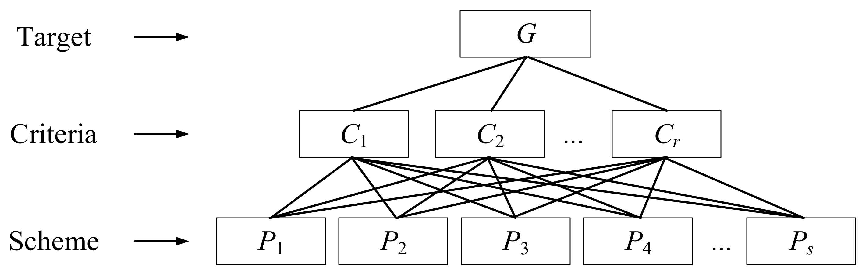
2.1. Existing Fuzzy Comprehensive Evaluation Method

The evaluation vector and value are calculated based on a factor set, membership matrix and weight vector in the existing method [23]. The factor set and evaluation set are $E=\{e_1,e_2,e_3,\dots ,e_m\}$ and $D=\{d_1,d_2,d_3,\dots ,d_n\}$, respectively. The fuzzy mapping from $E$ to $F(D)$ is established as: $f:E\to F(D)$, $\forall e_i\in E$, $e_i\to f(e_i)=r_{i1}/d_1+r_{i2}/d_2+\dots +r_{in}/d_n$ $(0\le r_{ij}\le 1, 1\le i\le m, 1\le j\le n)$. The fuzzy relation is induced by $f$ to calculate the membership matrix $R={(r_{ij})}_{m\times n}$ of factors. The ith row of $R$ represents the mapping result of fuzzy comprehensive evaluation on the ith factor. Different factors have different weights on the evaluation result; thus, it is necessary to construct corresponding weight vectors for all factors. Currently, the main methods for constructing weight vectors include expert estimation, delphi, weighted average, frequency distribution and analytic hierarchy process (AHP). Compared with other methods, the AHP makes decision according to the thinking mode of decomposition, comparative judgment and synthesis, which is more suitable for the decision−making problem of difficult−to−quantify prioritization with multi−objects and multi−criteria. The existing AHP divides the factors into three layers: target, criteria and scheme, as shown in Figure 1.

The weight of the target layer is set as 1, and it is assigned to different factors in the criteria layer. Each factor weight in the scheme layer comes from the assignment of each factor weight in the criteria layer. The final weight sum of each layer is 1. All factors in the criteria layer are compared in pairs to construct a comparison matrix $A_c={(a_{ij})}_{r\times r}$. The consistency of matrix $A_c$ is verified based on the consistency ratio $CR=\mu /RI$. If $CR<0.1$, $A_c$ is considered to have satisfactory consistency. Otherwise, $A_c$ needs to be modified. $RI$ is the average random consistency index, which is the average index of a large number of random reciprocal matrices of same order [24]. $\mu$ is the consistency index of $A_c$:

$$\mu =\frac{{\lambda }_{\max }-r}{r-1}=\frac{1}{r(r-1)}{\displaystyle \sum _{1\le i<j\le r}({\epsilon }_{ij}+{\epsilon }_{ji}-2)}=\frac{1}{r(r-1)}{\displaystyle \sum _{\begin{array}{l}i\ne j\\ i,j=1\end{array}}^r({\epsilon }_{ij}-1)}$$

(1)

${\lambda }_{\max }$ is the largest eigenvalue of $A_c$, $w_c={(w_1,w_2,\dots ,w_r)}^T$ is the eigenvector of $A_c$ corresponding to ${\lambda }_{\max }$, ${\mathit{W}}_c={(w_{ij})}_{r\times r}={(w_i/w_j)}_{r\times r}$ is the consistency matrix, ${\epsilon }_{ij}=a_{ij}/w_{ij}$, ${\epsilon }_{ij}>0$, ${\epsilon }_{ij}=1/{\epsilon }_{ji}$, if ${\epsilon }_{ij}=1$, and there is no error in the comparison matrix $A_c$. $w_c={(w_1,w_2,\dots ,w_r)}^T$ is calculated based on the comparison matrix meeting consistency requirements. The normalized $w_{ci}, i=1,2,\dots ,r$ are used as the weights of thecriteria layer factors. To calculate the weights of the scheme layer factors, the comparison matrix $A_{pi}$ corresponding to each $C_i, i=1,2,\dots ,r$ needs to be calculated. Then, the weight $w_{pi}$ of factor $P_i$ is obtained by weight assignment from each $C_i$ according to Equation (2).

$$w_{pi}={\displaystyle \sum _{j=1}^r{w}_{pij}}$$

(2)

In $w_{pij}, j=1,2,\dots ,r$ is the weight component of $P_i$ from each $C_i$. The weight values corresponding to all factors are used to construct the weight vector $w=(w_1,w_2,\dots ,w_m)$. According to Equation (3), the final fuzzy comprehensive evaluation vector $S$ is calculated to realize the object evaluation based on multiple factors.

$$S=w\mathit{R}$$

(3)

2.2. Improved Fuzzy Comprehensive Evaluation Method Based on Relative Hierarchy Factor Set

The FCE is improved by constructing a hierarchical tree model without a cross and a relative factor set with positive and negative effects, a forward constructing weight vector, and an inverse calculating membership matrix and comprehensive evaluation value.

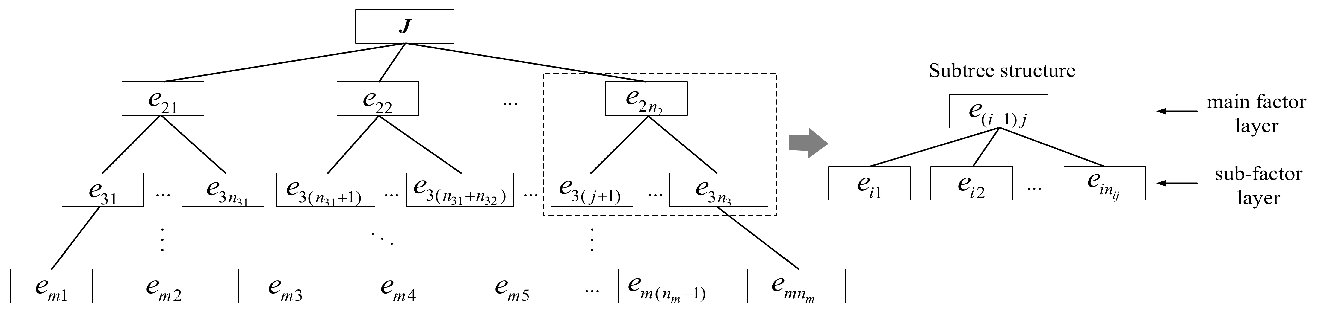
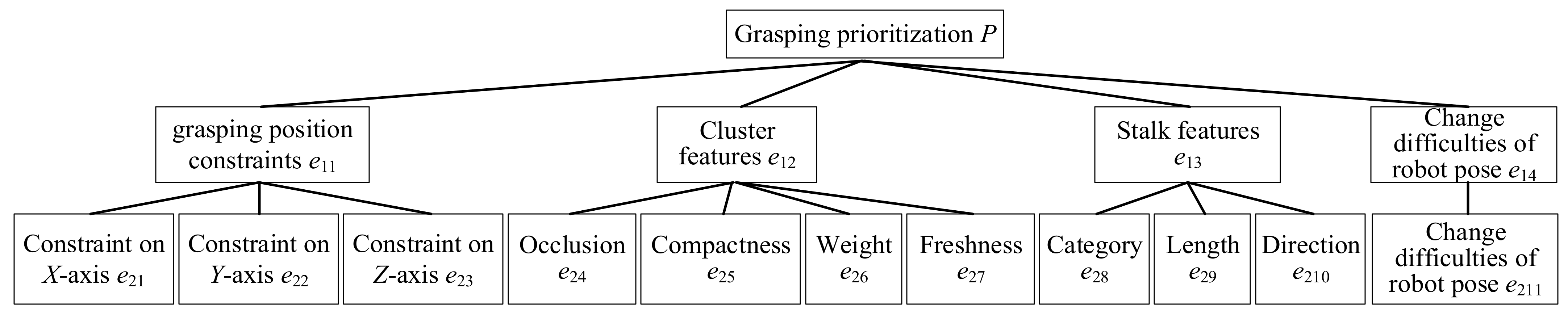
2.2.1. Hierarchical Tree Model without a Cross

A hierarchical tree model without a cross is constructed by analyzing multiple factors affecting the evaluation results, as shown in Figure 2. The evaluation vector $J$ is determined by multiple factors in the first layer, and the evaluation result of each factor is determined by multiple factors in the next layer. Each factor can only affect the evaluation result of one factor in the previous layer. Then, the hierarchical tree model without a cross is formed by an analogy. $m$ is number of layers, in $n_i, i=1,2,\dots ,m$ is the number of factors in layer $i$ and in $n_1=1$, $n_{ij}$ represents the number of factors in the sub−factor layer of the $j^{\mathrm{th}}$ subtree structure in the $i^{\mathrm{th}}$ layer of the model. In $j=1,2,\dots ,k_i$, $k_i$ is the number of subtree structures in the $i^{\mathrm{th}}$ layer of the model and $k_i=n_{i-1}$. The model is composed of subtree structures. The first layer of the subtree structure is the main factor layer and the second layer is the sub−factor layer. There is more than one subtree structure in each of the two layers of the model, and there is no cross between the subtree structures.

2.2.2. Relative Factor Set with Positive and Negative Effects

For the model with $m$ layers, the absolute factor set of the $g^{\mathrm{th}}$ evaluation object is represented by vector $E_g=(e_{21g},e_{22g},\dots ,e_{2n_{2}g},e_{31g},e_{32g},\dots ,e_{3n_{3}g},\dots ,e_{m{n}_{m}g})$ and $g=1,2,\dots ,b$. $b$ is the number of objects to be evaluated in an image. According to Equation (4), the same factors of different objects are normalized to calculate the relative factor vector ${{\mathit{E}}^{\prime }}_g=({e^{\prime }}_{21g},{e^{\prime }}_{22g},\dots ,{e^{\prime }}_{2n_{2}g},{e^{\prime }}_{31g},{e^{\prime }}_{32g},\dots ,{e^{\prime }}_{3n_{3}g},\dots ,{e^{\prime }}_{\mathrm{m}{n}_{\mathrm{m}}g})$ of multiple objects in an image. $s=\max (n_i),i=1,2,\dots ,m$, the $\max (e_{ijg})$ and $\min (e_{ijg})$ are the maximum and minimum values respectively when $g=1,2,\dots ,b$.

$${e^{\prime }}_{ijg}=\frac{e_{ijg}-\min (e_{ijg})}{\max (e_{ijg})-\min (e_{ijg})},i=2,3,\dots ,m;j=1,2,\dots ,s$$

(4)

The higher the factor value, the lower the priority order, which is called the negative effect. Otherwise, it is called the positive effect. According to the positive or negative effect of each factor on prioritization, the effect vector $P_N=(p_1,p_2,p_3,\dots p_a), a={{\displaystyle \sum }}_{i=2}^m{n}_i$ is constructed, and $p_i\in \left\{-1,1\right\}$. The positive and negative effects of factors correspond to $p_i=1$ and $p_i=-1$, respectively. Performing the Hadamard product for relative factor vector ${{\mathit{E}}^{\prime }}_g$ and effect vector $P_N$, the relative factor set with positive and negative effects can be represented by vector ${{\mathit{E}}^{″}}_g$ and calculated according to Equation (5).

$${{\mathit{E}}^{″}}_g=P_N\circ {{\mathit{E}}^{\prime }}_g$$

(5)

2.2.3. Forward Construction of Weight Vector

According to the hierarchical tree model without a cross, the weight vector is constructed using a forward transfer method from top to bottom. The sum of the weights in each layer of the model is 1, and the weight of each sub−factor comes from the weight assignment of the factors in the previous layer. If the weight in the main factor layer of the $j^{\mathrm{th}}$ subtree structure in the $i^{\mathrm{th}}$ layer of the model is $v_{(i-1)j}$, the sum of the sub−factor weights $v_{ijk}$ belonging to this main factor is $v_{(i-1)j}={{\displaystyle \sum }}_{k=1}^{n_{ij}}{v}_{ijk}$.

(1)

Construction of a comparison matrix

The comparison matrix $A_{ij}={(a_{ij})}_{n_{ij}\times n_{ij}}$ of the $j^{\mathrm{th}}$ subtree structure in the $i^{\mathrm{th}}$ layer of the model is constructed using the way of factor comparison in pairs. If the importance of $e_i$ compared with $e_j$ is $a_{ij}$, then the importance of $e_j$ compared with $e_i$ is $a_{ji}=1/a_{ij}$.

(2)

Consistency verification of comparison matrix

The ideal comparison matrix $A_{ij}$ should be a consistency matrix satisfying $a_{ij}{a}_{jk}=a_{ik}, (1\le i,j,k\le n_{ij})$. However, because construction of the comparison matrix is affected by subjective decision making, the consistency of the actual comparison matrix may not meet requirements. Therefore, it is necessary to verify the consistency of $A_{ij}$ and adjust the consistency based on the verification results. In this paper, the existing consistency verification method is improved by using the mathematical expectation $E(\mu )$ of $\mu$ as the average random consistency index of $A_{ij}$. Based on the normal distribution of $\mu$, the upper critical value of the consistency index of $A_{ij}$ is calculated and used as the consistency satisfaction value to improve verification accuracy. ${\epsilon }_{ij}$ is uniquely determined by the comparison matrix $A_{n\times n}$ and consistency matrix $W$ of $A$.

In a certain precision range, the same eigenvector $w={(w_1,w_2,\dots ,w_n)}^T$ and $W$ correspond to an infinite positive reciprocal matrix $A_i,i=1,2,3,\dots$. Therefore, according to Equation (6), $A_i$ can be calculated based on random perturbation of the same consistency matrix $W$.

$$A_i=W\circ F$$

(6)

$F={({\epsilon }_{ij})}_{n\times n}$ is the random perturbation matrix. When ${\epsilon }_{ij}\ge 1$, its probability density function $f(x)$ obeys some kind of semi−normal distribution. When $0<{\epsilon }_{ij}\le 1$, $f(x)$ is calculated based on the reciprocal of therandom variable. When ${\epsilon }_{ij}<0$, $f(x)$ is 0. Then:

$$f(x)=\left\{\begin{array}{ll}0& x\le 0\\ \frac{1}{x^2\sqrt{2\pi }\sigma }{e}^{-\frac{{(\frac{1}{x}-1)}^2}{2{\sigma }^2}}& 0<x\le 1\\ \frac{1}{\sqrt{2\pi }\sigma }{e}^{-\frac{{(x-1)}^2}{2{\sigma }^2}}& x\ge 1\end{array}\right.$$

(7)

Therefore, the relationship that ${\epsilon }_{ij}$ and ${\epsilon }_{ji}$ are reciprocal and have the same probability is reflected in the probability distribution. ${\epsilon }_{ij}$ are regarded as independent random variables with the same distribution. $\mu$ obeys the normal distribution approximately. Then, the mathematical expectation $E(\mu )$ of $\mu$ can be calculated according to Equation (8).

$$\begin{array}{c}E\left(\mu \right)=\frac{1}{n(n-1)}\sum _{\begin{array}{l}i\ne j\\ i,j=1\end{array}}^{n}E({\epsilon }_{ij}-1)\hfill \\ =\frac{1}{n(n-1)}{\displaystyle \sum }_{\begin{array}{l}i\ne j\\ i,j=1\end{array}}^n[{{\displaystyle \int }}_0^1(x-1)\frac{1}{x^2\sqrt{2\pi }\sigma }{e}^{-\frac{{(\frac{1}{x}-1)}^2}{2{\sigma }^2}}dx+{{\displaystyle \int }}_1^{+\infty }(x-1)\frac{1}{\sqrt{2\pi }\sigma }{e}^{-\frac{{(x-1)}^2}{2{\sigma }^2}}dx]\hfill \\ =\frac{1}{n(n-1)}\sum _{\begin{array}{l}i\ne j\\ i,j=1\end{array}}^n{{\displaystyle \int }}_1^{+\infty }(x+\frac{1}{x}-2)\frac{1}{\sqrt{2\pi }\sigma }{e}^{-\frac{{(x-1)}^2}{2{\sigma }^2}}dx\hfill \\ ={{\displaystyle \int }}_1^{+\infty }(x+\frac{1}{x}-2)\frac{1}{\sqrt{2\pi }\sigma }{e}^{-\frac{{(x-1)}^2}{2{\sigma }^2}}dx\hfill \end{array}$$

(8)

$E(\mu )$ can be regarded as the average random consistency index of $A$. According to normal distribution, $E(\mu )+1.29\sqrt{D(\mu )}$ is calculated based on $E(\mu )$ and the mathematical variance $D(\mu )$, and is regarded as the upper critical value of the consistency index of $A$ to replace the original consistency satisfaction value $0.1RI$. When $\mu \le E(\mu )+1.29\sqrt{D(\mu )}$, the comparison matrix is considered to have satisfactory consistency.

(3)

Weight calculation based on a comparison matrix

If comparison matrix $A$ has the largest eigenvalue ${\lambda }_{\max }$, and if $w={(w_1,w_2,\dots ,w_n)}^T$ is the eigenvector of $A$ corresponding to ${\lambda }_{\max }$, then:

$$w_i=\sqrt[n]{{\displaystyle \prod _{j=1}^n{a}_{ij}}} ,i=1,2,\dots ,n$$

(9)

The eigenvector is normalized to be used as the weight coefficient of the sub−factor layer of the subtree structure:

$${w^{\prime }}_i=\frac{w_i}{{{\displaystyle \sum }}_{i=1}^n{w}_i}$$

(10)

The weight of the sub−factor layer of the subtree structure comes from the assignment of the weight in the main factor layer, and $v_{(i-1)j}={{\displaystyle \sum }}_{k=1}^{n_{ij}}{v}_{ijk}$. Therefore, according to the weight coefficient vector $w^{\prime }={({w^{\prime }}_1,{w^{\prime }}_2,\dots ,{w^{\prime }}_n)}^T$, the corresponding weight is:

$$v_{ijk}=v_{(i-1)j}{w^{\prime }}_k ,k=1,2,\dots ,n$$

(11)

$v_{11}=1$, and $n=n_{ij}$ is the number of factors in the sub−factor layer of the $j^{\mathrm{th}}$ subtree structure in the $i^{\mathrm{th}}$ layer of the model and is the corresponding weight vector order, and $i=2,3,\dots ,m$. Then, the weight vector in the sub−factor layer of the $j^{\mathrm{th}}$ subtree structure in the $i^{\mathrm{th}}$ layer of the model is:

$$V_{ij}=(v_{ij1},v_{ij2},\dots ,v_{ij{n}_{ij}})$$

(12)

From the first layer, the weight vectors of all subtree structures in the model are calculated from top to bottom:

$$V={(V_{ij})}_{sum\times 1} , sum={\displaystyle \sum _{i=1}^m{\displaystyle \sum _{j=1}^{k_i}{\displaystyle \sum _{p=1}^{n_{ij}}1}}}$$

(13)

2.2.4. Inverse Calculation of the Membership Matrix and Comprehensive Evaluation Value

Compared with the existing method calculating the evaluation vector based on all factors directly, from the membership matrix of the last layer, the evaluation vector of the main factor in each subtree structure is calculated from bottom to top based on the constructed hierarchical tree model without a cross in this paper. Then, based on the evaluation vector of the main factor in the $j^{\mathrm{th}}$ subtree structure, the membership matrix of the sub−factor in the ${(j-1)}^{\mathrm{th}}$ subtree structure is calculated. The evaluation vector is set to $D=(d_1,d_2,d_3,\dots ,d_N)$, and the membership matrix of all factors in the last layer ($m^{\mathrm{th}}$ layer) of the model is:

$$R=\left[\begin{array}{l}{R}_{m1}\\ R_{m2}\\ \cdots \\ R_{m{k}_m}\end{array}\right]=\left[\begin{array}{ccccc}{r}_{11}& r_{12}& r_{13}& \cdots & r_{1N}\\ r_{21}& r_{22}& r_{23}& \cdots & r_{2N}\\ \cdots & & & & \\ r_{n_{m}1}& r_{n_{m}2}& r_{n_{m}3}& \cdots & r_{n_{m}N}\end{array}\right]$$

(14)

$R$ is composed of the membership matrices $R_{mj}, j=1,2,\dots ,k_m$ of the $k_m$ subtree structures in the $m^{\mathrm{th}}$ layer. The membership matrix of the $j^{\mathrm{th}}$ subtree structure in the $m^{\mathrm{th}}$ layer of the model is: $R_{mj}={(r_{ij})}_{n_{mj}N}$, and ${{\displaystyle \sum }}_{j=1}^N{r}_{ij}=1$. Each row of the membership matrix represents the probabilities that the object belongs to different values of the evaluation vector in factor $e_{ij}$. The comprehensive evaluation vector $J_{(m-1)q}$ corresponding to the $q^{\mathrm{th}}$ factor of the ${(m-1)}^{\mathrm{th}}$ layer of the model is calculated based on $R_{mj}$:

$$J_{(m-1)q}=V_{mj}{R}_{mj}, q=1,2,\dots ,n_{m-1}$$

(15)

$n_{m-1}=k_m$. If the sub−factors of the $j^{\mathrm{th}}$ subtree structure in the ${(m-1)}^{\mathrm{th}}$ layer of the model correspond to the $a^{\mathrm{th}}$ to $b^{\mathrm{th}}$ factors of the ${(m-1)}^{\mathrm{th}}$ layer of the model, the membership matrix $R_{(m-1)j}$ of the $j^{\mathrm{th}}$ subtree structure in the ${(m-1)}^{\mathrm{th}}$ layer of the model is calculated based on $J_{(m-1)q}$, according to Equation (16).

$$R_{(m-1)j}={\left[J_{(m-1)a} J_{(m-1)(a+1)} J_{(m-1)(a+2)} \cdots J_{(m-1)b}\right]}^T$$

(16)

Then, according to Equations (15) and (16), the comprehensive evaluation vector $J$ of the top layer is calculated by iterating from the lower to the top layer:

$$J=V_{21}{R}_{21}$$

(17)

In the fuzzy comprehensive evaluation for grasping prioritization, the value in $J$ is the probability that each object belongs to the corresponding grasping prioritization. Therefore, the prioritization corresponding to the maximum value in $J$ is selected as the prioritization for the grasping object. The final evaluation value is: $d=d_{ma}$. $ma$ is the index corresponding to the maximum value in $J$, and $J_{ma}=\max (J_i), i=1,2,\dots ,N$.

2.3. Prioritizing Robotic Grasping for Stacked Fruit Clusters Based on Improved FCE

The process of prioritizing robotic grasping for stacked fruit clusters based on improved FCE is shown in Figure 3. According to the features of stacked fruit clusters in the image, such as fitting the line segments of stalks, stalk depths, stalk pixels, cluster area, centroid of cluster, centroids of berries and number of berries, and motion features of low-DOF parallel robot, the factors affecting grasping prioritization are calculated. The improved FCE is used to evaluate the grasping prioritization accurately.

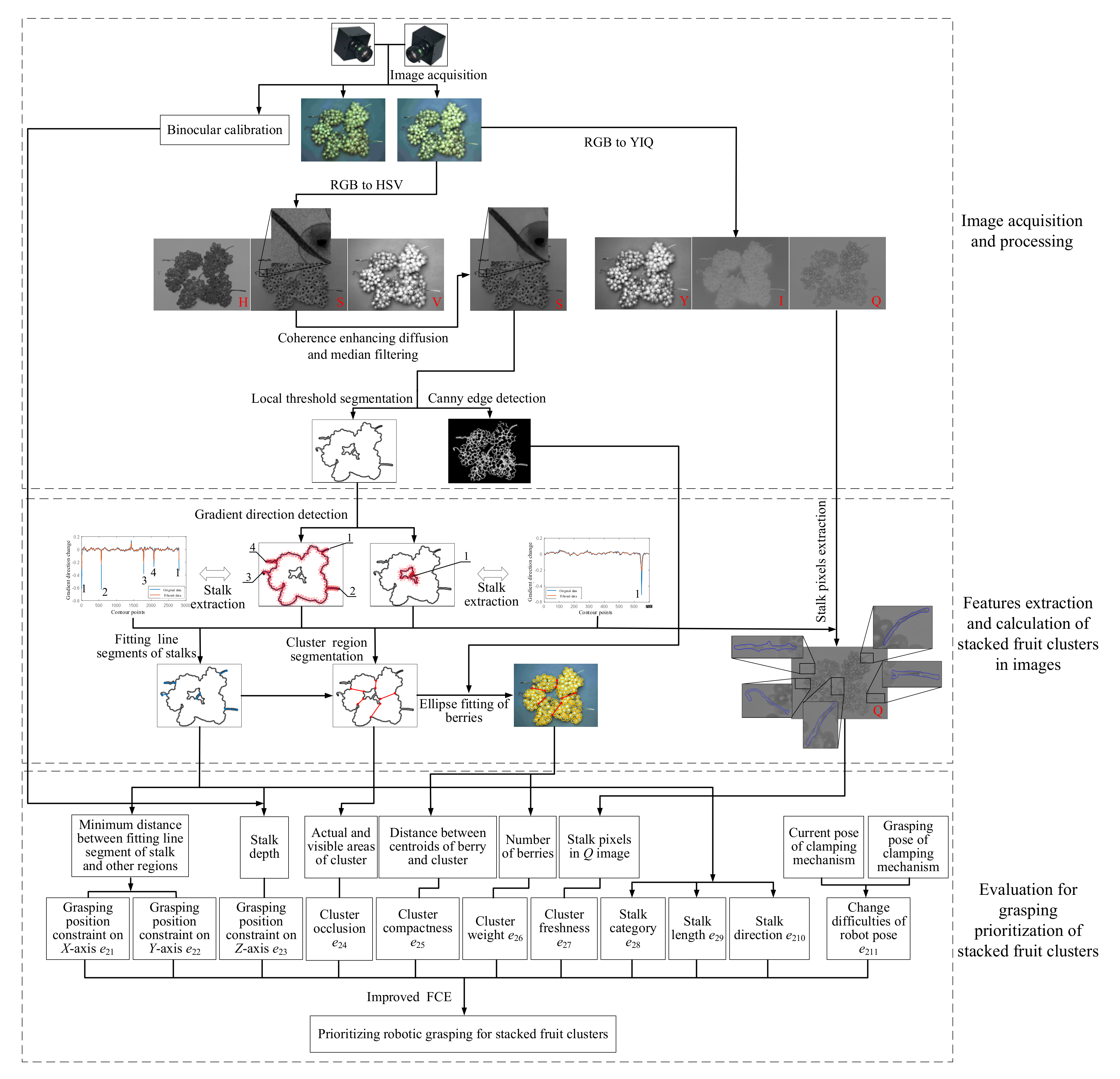
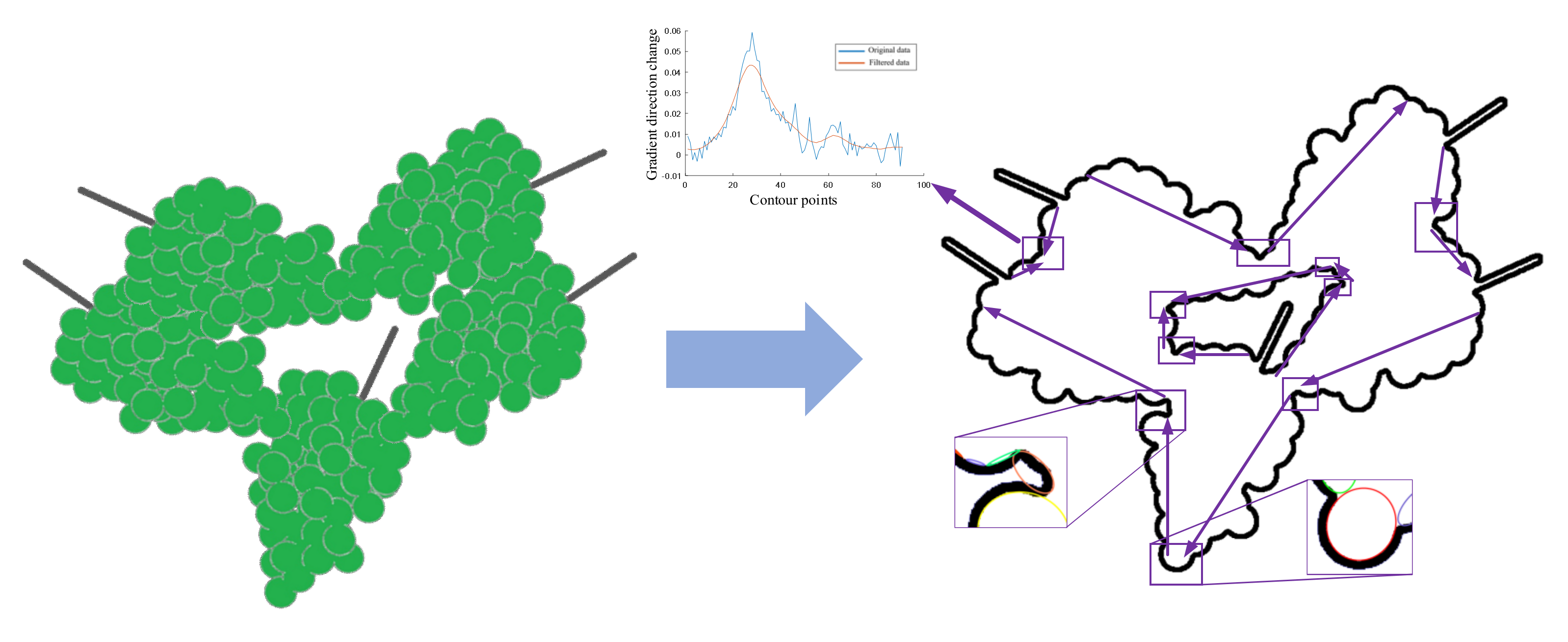
2.3.1. Image Acquisition and Processing

To obtain the depth and color features of the fruit clusters, two cameras are used to obtain RGB images of the stacked fruit clusters, and the camera calibration method based on a single calibration plate is used [25,26]. Under the same lighting conditions, compared with other regions, the protruding and smooth region of the berry ball in the optical axis direction is more likely to be white in the image due to overexposure. Because the color can be regarded as the mixture of spectral color and white, the S image in the HSV (hue, saturation, value) color model can represent the degree that the color is close to the spectral color or white. Therefore, to increase the contrast between the berry and the background in the image and to retain more detailed features of the stacked fruit clusters, the S image is used to extract contour of the fruit clusters. According to the texture features of the fruit clusters, the coherence enhancing diffusion [27] and median filtering are used to preprocess the S image for sharpening the image edges and reducing the effect of noise [28]. The binary image of the fruit cluster contours is obtained by local threshold segmentation and Canny edge detection. In addition, compared with berry regions, the color of the stalk regions in the images of the fruit clusters with different freshness changes greatly and is less affected by overexposure and specular reflection, which is more suitable to analyze fruit cluster freshness. As shown in Figure 4a, the color of the stalk changes from green to brown with time. Compared with the RGB color model that each image contains only one basic color and cannot describe the color change, the Q image in the quadrature−phase color model can represent the change of color from purple to yellow green. It is more suitable to extract the stalk color feature representing fruit cluster freshness, as shown in Figure 4b.

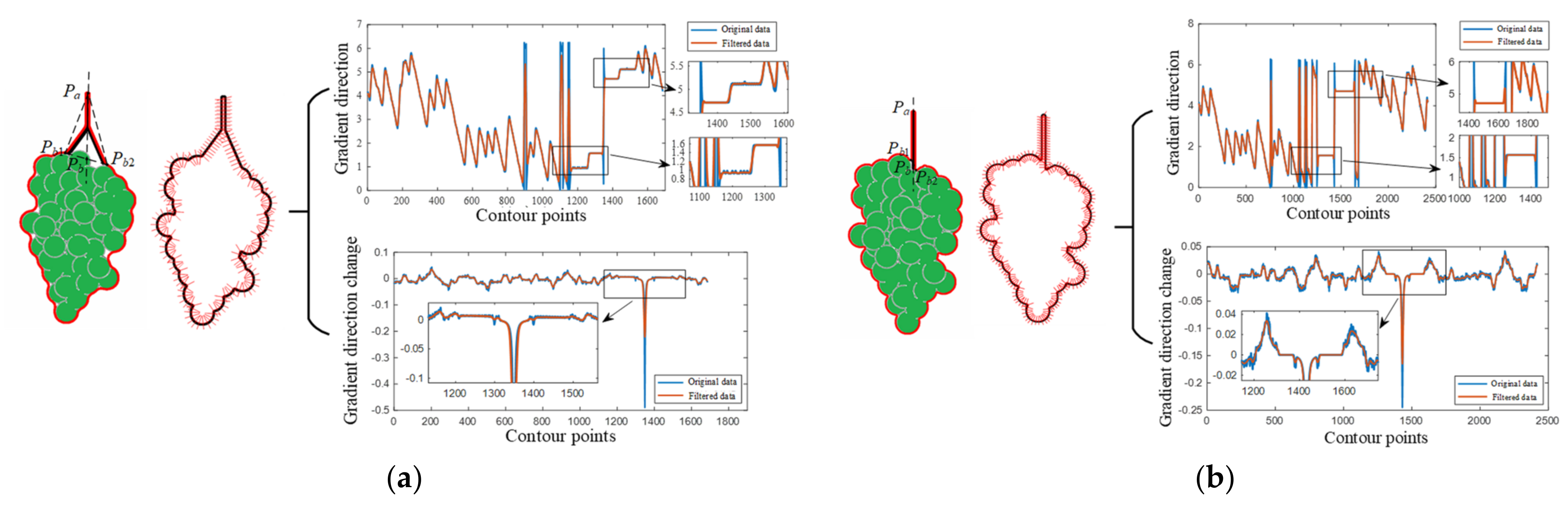
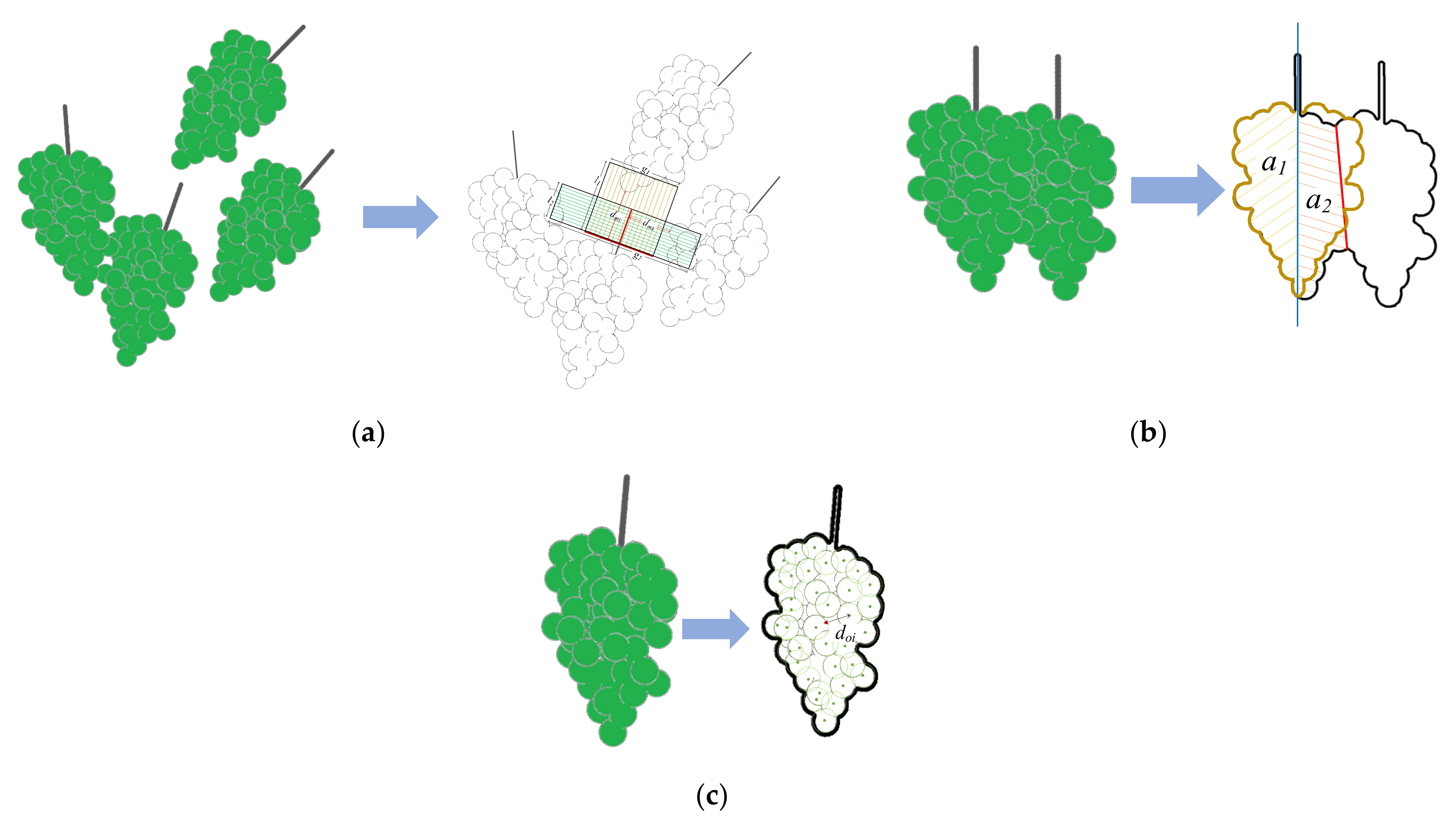
2.3.2. Features Extraction and Calculation of Stacked Fruit Clusters in Images

The positions of the stalk contours are detected according to gradient direction changes of the cluster contour. Compared with the gradient direction changes of other regions, the direction of the stalk endpoint changes greatly and is located in the trough of the gradient direction change curve, as shown in Figure 5. Therefore, the position of the stalk endpoint $p_a$ can be detected based on the curve extremum at a certain threshold. According to the gradient direction changes of the points near $p_a$, the stalk category is determined. If there are two regions with small direction changes on the left and right of $p_a$, there is a node in the stalk. Otherwise, there is no node in the stalk. The contour intersections of the stalk and cluster for the stalk with a node and stalk without a node are located in the positions of second and third peaks near the trough $p_a$, respectively. The midpoint $p_b$ of intersections $p_{b1}$ and $p_{b2}$ is another endpoint of the stalk. The line segment of the stalk is fitted based on $p_a$ and $p_b$; the stalk length and direction, the distances between the fitting line segment of the stalk and other regions are calculated. The ROI (region of interest) for the stalk is extracted based on $p_a$, $p_{b1}$ and $p_{b2}$, and the stalk region is extracted based on local threshold segmentation. Then, according to the RGB image obtained by the left and right cameras and the Q image obtained by image transformation, the depth and color features of the stalk are extracted, respectively.

The stalk contours are removed based on $p_{b1}$ and $p_{b2}$. The constraints for detecting segmentation points of the cluster regions are constructed according to the global direction changes of contours, fitted ellipses of local contours, and gradient directions, as shown in Figure 6. The extremum of the global direction change curve of a fruit cluster contour mainly corresponds to the contour intersections of the stalk and cluster and the bottom contour of cluster. Compared with fruit cluster contour, the contour global directions of different clusters are different, and the direction changes in the intersections of the cluster contours are obvious. Therefore, the candidate positions of cluster segmentation points can be extracted according to the extremums of global direction change curves of cluster contours. The candidate positions include the intersections of different cluster contours, the bottom contours of clusters, and the berry contours on the cluster edges. Compared with the intersections of the different cluster contours, the centers of the fitting circles of the berry contours on the edges of the clusters are inside the cluster contours. Because the shape of the berry is not a standard circle and the cluster contour is composed of berry contours, there is a difference between the center position of the fitting circle of the berry contour on the cluster contour and the actual center position. Therefore, the centers of the arcs corresponding to the berry contours on the cluster contour are calculated based on ellipse fitting. The relationships between the fitted ellipse centers of the arcs corresponding to the candidate positions and cluster contour are judged to purify the candidate positions. If the ellipse center is inside the cluster contour, the corresponding candidate position is removed. Otherwise, it is retained. On purified candidate positions, the gradient direction changes of the contour points are detected, and the extremums of the change curves filtered by a small convolution kernel are calculated as the segmentation points. The matching of segmentation points for cluster segmentation has the following constraints: (1) The Euclid distance between two points is the smallest. (2) There is no intersection between the line segment composed of two points and the cluster contour. The constraint (2) is judged first. If the constraint (2) is satisfied, the constraint (1) is calculated based on the distance matrix, and the closest two points are taken as the matching point pairs. The line segment composed of matching point pairs is the segmentation line of the cluster region. The actual and visible areas of the clusters and the centroids of the clusters are calculated based on the segmented cluster regions. In the edge binary image of a single cluster region, the berry contours are fitted to ellipses for calculating the centroids and number of berries.

2.3.3. Evaluation for Grasping Prioritization of Stacked Fruit Clusters

Based on the factors affecting grasping prioritization of stacked fruit clusters, the hierarchical tree model with three layers is constructed, as shown in Figure 7.

The factors include four categories: grasping position constraints $e_{11}$, cluster features $e_{12}$, stalk features $e_{13}$ and change difficulties of robot pose $e_{14}$, and they are all relative factors of multiple objects in an image. The grasping position constraints include the constraints on the X-axis, Y-axis and Z-axis denoted as $e_{21}$, $e_{22}$ and $e_{23}$, correspondingly. According to the minimum distances $d_{mx}$ and $d_{my}$ between the fitting line segment of stalk and other regions in the directions perpendicular and parallel to the fitting line segment, the finger width $g$ and length $l$ of the clamping mechanism, the grasping position constraints on the X-axis and Y-axis are defined. As shown in Figure 8a, if there are other regions in the calculation area, the absolute factor values of the grasping position constraints are:

$$e_{21}=2d_{mx}-2g-w$$

(18)

$$e_{22}=d_{m\mathrm{y}}-l$$

(19)

$w$ is the opening width of the clamping mechanism. The size of the calculation area is calculated based on Equations (20) and (21). The $l_p$ is the length of the stalk fitting line segment. If there is no other region in the calculation area, the calculation area is extended to the image boundary.

$$g_1=2g+w, l_1=2l$$

(20)

$$g_2=4g+w, l_2=\left\{\begin{array}{ll}l,& l_p\le l\\ l_p,& l_p>l \end{array}\right.$$

(21)

According to Equation (22), the grasping position constraint on the Z-axis is calculated based on the depths $d_a$ and $d_b$ of the stalk endpoints from the detection plane. To make the fitting line segment of the midpoint of the stalk coincide with the finger midpoint of the clamping mechanism, the finger height $h$ of the clamping mechanism is used to calculate the grasping position constraint.

$$e_{23}=\frac{(d_a+d_b)}{2}-\frac{h}{2}$$

(22)

The cluster features include four sub−factors: occlusion, compactness, weight and freshness, denoted as $e_{24}$, $e_{25}$, $e_{26}$ and $e_{27}$, correspondingly. The occlusion is calculated based on the cluster area, as shown in Figure 8b. The red line in Figure 8b is the segmentation line of the cluster region. The cluster region is divided into left and right regions based on the stalk fitting line. The larger area in the left and right regions is taken as the half actual area of the cluster region (yellow area in Figure 8b). Then, the ratio of the visible area $a_1+a_2$ to actual area $2a_1$ is taken as the occlusion:

$$e_{24}=\frac{a_1+a_2}{2a_1}$$

(23)

As shown in Figure 8c, according to Equation (24), the compactness is calculated based on the distance $d_{oi}$ between centroids of the berry and cluster in the segmented cluster region. $n$ is the number of berries. The centers of fitting ellipses are calculated and used as the centroids of the berries. The fitting ellipses of the berries are obtained based on the least−squares method in the edge binary image of a single cluster region [29,30]. According to Equation (25), the centroid coordinate $(x_o,y_o)$ of the cluster is calculated. $(x,y)$ is the contour point coordinate of the cluster, and $f(x,y)$ is the contour point gray value.

$$e_{25}=\frac{{\displaystyle \sum _{i=1}^n{d}_{oi}}}{n^2}$$

(24)

$$\left\{\begin{array}{l}{x}_o={\displaystyle \sum xf(x,y)}/{\displaystyle \sum f(x,y)}\\ y_o={\displaystyle \sum yf(x,y)}/{\displaystyle \sum f(x,y)}\end{array}\right.$$

(25)

The berry average weight $k_a$ obtained from a large number of experiments is used to estimate the weight of the fruit cluster in the image:

$$e_{26}=n{k}_a$$

(26)

The fruit cluster freshness is defined according to the stalk color and is calculated based on average gray value of the stalk region in the Q image according to Equation (27). $n_R$ is the number of points in the stalk region, and $f(x,y)$ is the point gray value.

$$e_{27}=\frac{{\displaystyle \sum f(x,y)}}{n_R}$$

(27)

The stalk features include three sub−factors: category, length and direction denoted as $e_{28}$, $e_{29}$ and $e_{210}$, correspondingly. As shown in Figure 9, the stalk is divided into two categories: stalk with a node and stalk without a node. The skeleton of the stalk with a node can be fitted to the line segments with the herringbone. The skeleton of the stalk without a node can be fitted to a line segment. According to the relationship between the line segments of the skeleton and $l$, the stalk can be further divided into six categories: short $AB$ stalk without node, long $AB$ stalk without node, short $AB$ stalk with node, long $AB$ stalk with node, short $EB$ stalk with node and long $EB$ stalk with node. Then, the absolute factor value of the stalk category is:

$$e_{28}=\left\{\begin{array}{l}1, l_{A^{\prime }{B}^{\prime }}\ge l \mathrm{and} \mathrm{without} \mathrm{node}\\ 2, l_{A^{\prime }{B}^{\prime }}<l \mathrm{and} \mathrm{without} \mathrm{node}\\ 3, l_{A^{\prime }{B}^{\prime }}\ge l \mathrm{and} \mathrm{with} \mathrm{node}\\ 4, l/2\le l_{A^{\prime }{B}^{\prime }}<l \mathrm{and} \mathrm{with} \mathrm{node}\\ 5, l_{A^{\prime }{B}^{\prime }}<l/2 \mathrm{and} l_{E^{\prime }{B}^{\prime }}\ge l \mathrm{and} \mathrm{with} \mathrm{node}\\ 6, l_{A^{\prime }{B}^{\prime }}<l/2 \mathrm{and} l_{E^{\prime }{B}^{\prime }}<l \mathrm{and} \mathrm{with} \mathrm{node}\end{array}\right.$$

(28)

$AB$, $BD$ and $BC$ are the line segments of the stalk skeleton. $r_2$ is the angular bisector of ∠DBC. $r_1$ is the tangent in the outermost point of the cluster contour. $E$ is the intersection point of $r_1$ and $r_2$. $l_{A^{\prime }{B}^{\prime }}$ and $l_{E^{\prime }{B}^{\prime }}$ are the projection lengths of the line segments $AB$ and $EB$ on the $X_w{Y}_w$ plane of the world coordinate system $O_w-X_w{Y}_w{Z}_w$, respectively.

The length and direction of the stalk are calculated based on the skeleton line segments of the stalk. If the endpoint coordinates of the skeleton line segments in $O_w-X_w{Y}_w{Z}_w$ are $A=(x_A,y_A,z_A)$,$B=(x_B,y_B,z_B)$ and $E=(x_E,y_E,z_E)$, the stalk length is:

$$e_{29}=\left\{\begin{array}{l}\sqrt{{(x_A-x_B)}^2+{(y_A-y_B)}^2+{(z_A-z_B)}^2}, e_{28}=1,2,3,4\\ \sqrt{{(x_B-x_E)}^2+{(y_B-y_E)}^2+{(z_B-z_E)}^2}, e_{28}=5,6\end{array}\right.$$

(29)

The stalk direction is represented by vector $e_{210}=(x_{210},y_{210},z_{210})$; thus, the absolute factor values of the stalk direction are:

$$x_{210}=\left\{\begin{array}{l}\frac{x_A-x_B}{e_{29}}, e_{28}=1,2,3,4\\ \frac{x_B-x_E}{e_{29}}, e_{28}=5,6\end{array}\right., y_{210}=\left\{\begin{array}{l}\frac{y_A-y_B}{e_{29}}, e_{28}=1,2,3,4\\ \frac{y_B-y_E}{e_{29}}, e_{28}=5,6\end{array}\right., z_{210}=\left\{\begin{array}{l}\frac{z_A-z_B}{e_{29}}, e_{28}=1,2,3,4\\ \frac{z_B-z_E}{e_{29}}, e_{28}=5,6\end{array}\right.$$

(30)

The absolute factor value for change difficulties of a robot pose denoted as $e_{211}$ is calculated according to the pose change $e_{211}=(x_{211},y_{211},z_{211},{\alpha }_{211},{\beta }_{211},{\theta }_{211})$ of the clamping mechanism from current pose $g$ to grasping pose $p$ [31]. Taking the 4 − R(2 − SS) parallel robot as an example, due to the motion constraint of the robot, the pose of the clamping mechanism includes the position $(x,y,z)$ in $O_w-X_w{Y}_w{Z}_w$ and rotation angle $\theta$ around the Z-axis. Therefore, the absolute factor value for the change difficulties of the robot pose can be simplified as $e_{211}=(x_{211},y_{211},z_{211},{\theta }_{211})$. $x_{211}=x_g-x_p$, $y_{211}=y_g-y_p$, $z_{211}=z_g-z_p$ and ${\theta }_{211}={\theta }_g-{\theta }_p$.

All absolute factor values are used to construct the absolute factor vector $E=(E_{11},E_{12},E_{13},E_{14})=(e_1,e_2,\dots ,e_{16})$ of the third layer in the prioritization model, including in $E_{11}=(e_{21},e_{22},e_{23})$, $E_{12}=(e_{24},e_{25},e_{26},e_{27})$, $E_{13}=(e_{28},e_{29},x_{210},y_{210},z_{210})$ and $E_{14}=(x_{211},y_{211},z_{211},{\theta }_{211})$. According to Equation (4), the absolute factor values are normalized to obtain ${\mathit{E}}^{\prime }$. Based on the positive and negative effects of the different factors on the grasping prioritization, the effect vector $P_N=(1,1,1,1,-1,-1,-1,-1,1,-1,-1,-1,-1,-1,-1,-1)$ is constructed. According to Equation (5), the relative factor set ${\mathit{E}}^{″}$ with positive and negative effects is constructed. Then, the corresponding weight vector is constructed from the top to the bottom of the model. The membership matrix and comprehensive evaluation value of the multi-layer factors are calculated from the bottom to the top of the model to evaluate the grasping prioritization of stacked fruit clusters.

3. Results

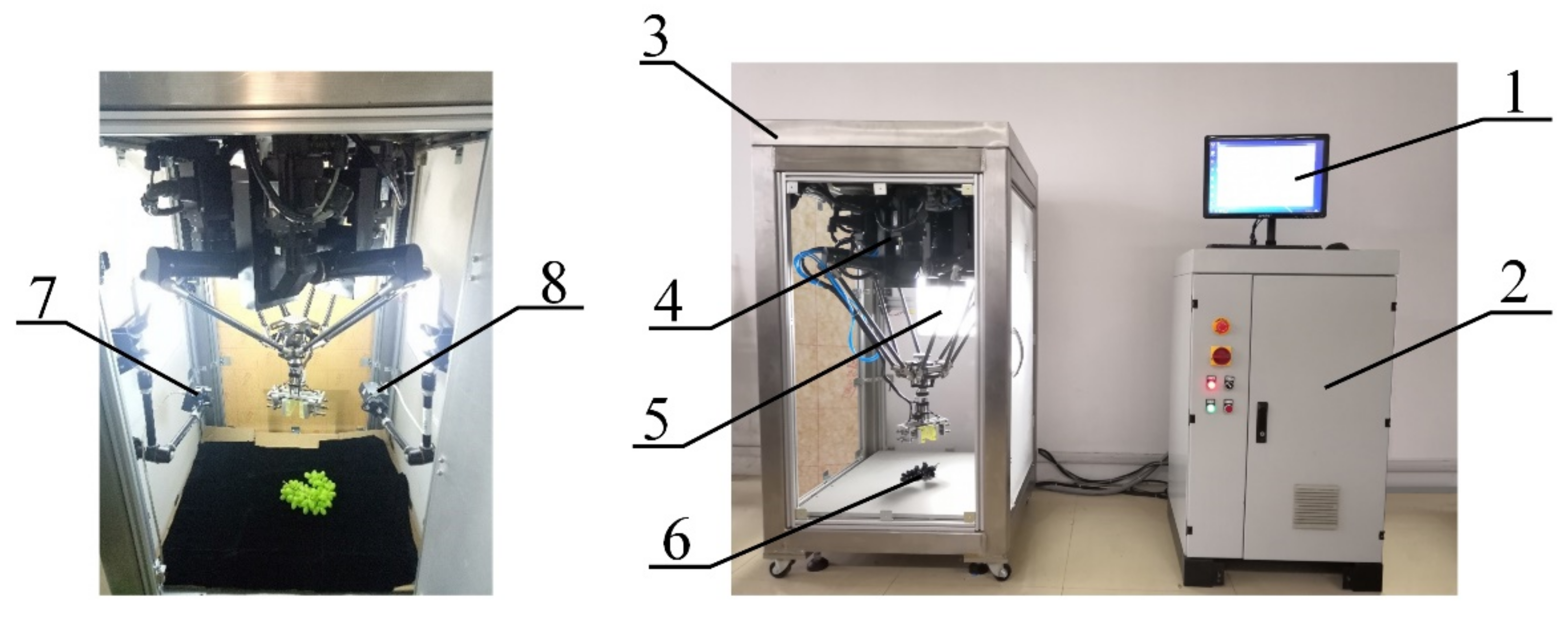
3.1. Experimental Platform

The experiments were performed in the self-developed automatic sorting system for stacked fruit clusters based on a 4 − R(2 − SS) parallel robot and machine vision, as shown in Figure 10. The images of the White Rosa grape clusters for the experiments were acquired by the left and right cameras. The hardware of the experiment included the calibration plate with $7\times 7$ circles with a diameter of 3.5 mm and spacing of 7 mm, the IntelICITM)i7−3770 CPU with 8GB memory, and a graphics card with NVIDIA GeForce GTX 1060 6GB. The flat light source with color temperature of 6600~7000 k was adopted to illuminate the fruit clusters.

3.2. Experimental Method

To verify the effectiveness and advantages of the proposed method, four group experiments were carried out based on the four factor categories in the second layer of the model. The White Rosa grape clusters were stacked in different ways. In the four group experiments, the main factor differences of the grasping prioritization among the images were the grasping position constraints, cluster features, stalk features and change difficulties of the robot pose. The improved FCE was compared with the existing FCE to verify the prioritization precision for the grasping stacked fruit clusters. The grasping prioritizations obtained by evaluation were compared with the prioritizations obtained by oft−repeated human detection to calculate the prioritization precision.

3.3. Experimental Results and Discussion

As shown in Figure 11, the original images for the experiments were divided into four groups with main differences of the grasping position constraints, fruit cluster features, stalk features and change difficulties of the robot pose. In each group of experiments, the 20 images of the stacked grape clusters were used for analysis. The factor values obtained in the four group experiments are shown in

Table 1. Experimental data with main differences of grasping position constraints.

Grasping Position Constraint on X-axis		Grasping Position Constraint on Y-axis		Grasping Position Constraint on Z-axis		Cluster Occlusion		Cluster Compactness		Cluster Weight
e21(mm)	e″21	e22(mm)	E″22	e23(mm)	e″23	e24(%)	e″24	e25(pixel)	e″25	e26(g)
−21.13	0.129	105.70	1.000	14.02	0.366	54.36	0.000	2.01	−0.101	635.55
−42.47	0.000	−7.47	0.000	31.34	0.630	63.55	0.591	1.99	−0.076	735.90
64.18	0.642	55.36	0.555	55.59	1.000	69.90	1.000	2.72	−1.000	479.45
75.96	0.713	78.94	0.764	41.28	0.782	61.18	0.439	2.34	−0.519	568.65
123.60	1.000	23.89	0.277	−10.01	0.000	56.37	0.129	1.93	0.000	769.35
Cluster Weight	Cluster Freshness		Stalk Category		Stalk Length		Stalk Direction
e″26	e27(pixel)	e″27	e28	e″28	e29(mm)	e″29	x210(mm)	x″210	y210(mm)	y″210
−0.538	89.15	0.000	1.00	0.000	68.70	0.789	−0.97	0.000	−0.24	−0.243
−0.885	93.33	−0.413	1.00	0.000	69.59	0.812	−0.89	−0.042	0.40	−0.673
0.000	90.84	−0.167	2.00	−0.500	38.52	0.000	0.92	−1.000	−0.36	−0.163
−0.308	99.26	−1.000	3.00	−1.000	76.77	1.000	0.79	−0.932	−0.60	0.000
−1.000	89.50	−0.035	1.00	0.000	61.24	0.594	−0.36	−0.321	0.89	−1.000
Stalk Direction		Change Difficulties of Robot Pose
z210(mm)	z″210	x211(mm)	x″211	y211(mm)	y″211	z211(mm)	z″211	θ211(°)	θ″211
−0.08	−1.000	−357.25	0.000	24.65	−0.786	−125.87	0.000	89.56	−0.781
−0.22	−0.272	235.64	−1.000	118.13	−1.000	489.53	−1.000	155.78	−1.000
−0.18	−0.460	145.20	−0.847	−318.90	0.000	337.20	−0.752	−99.45	−0.156
−0.15	−0.650	−65.73	−0.492	−44.82	−0.627	246.81	−0.606	−146.80	0.000
−0.27	0.000	−212.61	−0.244	57.88	−0.862	−33.76	−0.150	66.84	−0.706

,

Table 2. Experimental data with main differences of fruit cluster features.

Grasping Position Constraint on X-axis		Grasping Position Constraint on Y-axis		Grasping Position Constraint on Z-axis		Cluster Occlusion		Cluster Compactness		Cluster Weight
e21(mm)	e″21	e22(mm)	e″22	e23(mm)	e″23	e24(%)	e″24	e25(pixel)	e″25	e26(g)
31.99	0.381	21.15	0.073	21.82	0.355	77.28	0.722	2.58	−0.374	401.40
43.13	0.574	15.83	0.000	16.18	0.153	86.94	1.000	3.77	−1.000	869.70
67.71	1.000	47.73	0.440	29.01	0.614	52.24	0.000	2.21	−0.179	713.60
10.04	0.000	88.40	1.000	39.77	1.000	69.15	0.487	1.87	0.000	535.20
37.70	0.480	26.40	0.146	11.93	0.000	72.30	0.578	3.02	−0.605	613.25
Cluster Weight	Cluster Freshness		Stalk Category		Stalk Length		Stalk Direction
e″26	e27(pixel)	e″27	e28	e″28	e29(mm)	e″29	x210(mm)	x″210	y210(mm)	y″210
0.000	89.81	0.000	3.00	−1.000	84.53	1.000	0.71	−0.939	−0.70	−0.008
−1.000	108.23	−0.460	2.00	−0.500	38.67	0.000	0.57	−0.850	0.79	−1.000
−0.667	129.86	−1.000	2.00	−0.500	46.87	0.179	−0.69	−0.037	−0.71	0.000
−0.286	100.02	−0.255	1.00	0.000	79.54	0.891	−0.75	0.000	−0.64	−0.045
−0.452	115.50	−0.641	1.00	0.000	67.77	0.635	0.80	−1.000	0.58	−0.860
Stalk Direction		Change Difficulties of Robot Pose
z210(mm)	z″210	x211(mm)	x″211	y211(mm)	y″211	z211(mm)	z″211	θ211(°)	θ″211
−0.07	−1.000	15.64	−0.411	73.60	−0.702	108.95	−1.000	105.67	−1.000
−0.23	0.000	−112.97	−0.182	268.94	−1.000	−145.78	0.000	15.31	−0.671
−0.13	−0.663	−215.40	0.000	−146.32	−0.366	−78.25	−0.265	−89.76	−0.288
−0.16	−0.426	347.38	−1.000	−386.10	0.000	14.55	−0.629	−168.90	0.000
−0.14	−0.569	−46.80	−0.300	33.65	−0.641	−88.45	−0.225	57.25	−0.824

,

Table 3. Experimental data with main differences of stalk features.

Grasping Position Constraint on X-axis		Grasping Position Constraint on Y-axis		Grasping Position Constraint on Z-axis		Cluster Occlusion		Cluster Compactness		Cluster Weight
e21(mm)	e″21	e22(mm)	e″22	e23(mm)	e″23	e24(%)	e″24	e25(pixel)	e″25	e26(g)
26.84	0.132	53.81	0.632	−3.23	0.000	54.85	0.000	2.23	−0.333	691.30
15.81	0.000	43.21	0.524	12.83	0.187	59.57	0.364	2.75	−0.778	657.85
99.58	1.000	−8.17	0.000	43.65	0.546	63.52	0.668	1.84	0.000	524.05
88.46	0.867	89.90	1.000	82.68	1.000	54.91	0.005	3.01	−1.000	747.05
68.85	0.633	42.30	0.515	36.29	0.460	67.83	1.000	1.91	−0.060	635.55
Cluster Weight	Cluster Freshness		Stalk Category		Stalk Length		Stalk Direction
e″26	e27(pixel)	e″27	e28	e″28	e29(mm)	e″29	x210(mm)	x″210	y210(mm)	y″210
−0.750	101.50	−0.752	3.00	−0.400	87.41	1.000	0.64	−0.466	0.76	−1.000
−0.600	94.29	−0.350	6.00	−1.000	47.07	0.232	0.43	0.000	−0.85	0.000
0.000	88.01	0.000	2.00	−0.200	39.26	0.084	0.70	−0.594	0.65	−0.932
−1.000	91.36	−0.187	1.00	0.000	56.72	0.416	0.88	−1.000	−0.46	−0.242
−0.500	105.94	−1.000	4.00	−0.600	34.86	0.000	0.88	−1.000	−0.44	−0.256
Stalk Direction		Change Difficulties of Robot Pose
z210(mm)	z″210	x211(mm)	x″211	y211(mm)	y″211	z211(mm)	z″211	θ211(°)	θ″211
−0.09	−1.000	−99.65	−0.070	278.42	−1.000	−138.50	0.000	−78.24	0.000
−0.31	0.000	−10.31	−0.240	55.84	−0.585	98.75	−0.459	−55.33	−0.124
−0.30	−0.048	55.80	−0.366	−15.76	−0.451	378.91	−1.000	−26.70	−0.280
−0.15	−0.724	−136.20	0.000	44.85	−0.564	307.34	−0.862	94.36	−0.938
−0.19	−0.530	388.50	−1.000	−257.90	0.000	255.90	−0.762	105.80	−1.000

and

Table 4. Experimental data with main differences of change difficulties of robot pose.

Grasping Position Constraint on X-axis		Grasping Position Constraint on Y-axis		Grasping Position Constraint on Z-axis		Cluster Occlusion		Cluster Compactness		Cluster Weight
e21(mm)	e″21	e22(mm)	e″22	e23(mm)	e″23	e24(%)	e″24	e25(pixel)	e″25	e26(g)
22.48	0.000	26.78	0.379	−7.42	0.000	61.22	0.369	1.83	0.000	535.20
63.56	0.846	18.49	0.269	3.19	0.154	70.85	1.000	1.93	−0.105	713.60
52.16	0.611	57.89	0.793	61.27	1.000	64.03	0.553	2.78	−1.000	680.15
71.04	1.000	−1.73	0.000	37.76	0.658	58.30	0.178	2.04	−0.221	602.10
45.17	0.467	73.50	1.000	30.11	0.546	55.59	0.000	2.61	−0.821	434.85
Cluster Weight	Cluster Freshness		Stalk Category		Stalk Length		Stalk Direction
e″26	e27(pixel)	e″27	e28	e″28	e29(mm)	e″29	x210(mm)	x″210	y210(mm)	y″210
−0.360	100.27	−0.782	1.00	0.000	65.83	0.601	0.57	−0.912	−0.81	0.000
−1.000	99.02	−0.716	2.00	−0.500	39.95	0.000	−0.68	−0.126	−0.63	−0.136
−0.880	104.37	−1.000	2.00	−0.500	43.77	0.089	−0.88	0.000	−0.25	−0.424
−0.600	85.54	0.000	1.00	0.000	71.40	0.731	0.71	−1.000	−0.69	−0.089
0.000	92.33	−0.361	3.00	−1.000	82.99	1.000	−0.86	−0.014	0.49	−1.000
Stalk Direction		Change Difficulties of Robot Pose
z210(mm)	z″210	x211(mm)	x″211	y211(mm)	y″211	z211(mm)	z″211	θ211(°)	θ″211
−0.15	−0.886	367.25	−1.000	−157.98	−0.423	507.45	−1.000	−33.76	−0.386
−0.38	−0.078	−57.94	−0.436	−355.60	0.000	−167.89	0.000	64.91	−0.794
−0.40	0.000	−387.30	0.000	98.67	−0.973	−33.68	−0.199	114.60	−1.000
−0.12	−1.000	218.60	−0.803	102.74	−0.981	336.30	−0.747	−126.87	0.000
−0.14	−0.935	14.70	−0.533	111.45	−1.000	77.89	−0.364	−88.35	−0.160

. The data in the tables are the absolute and relative factor values in a random image of each group.

According to Equations (31)–(33), the difference ratio $R{P}_i$, and average difference ratios $\overline{R{P}_{210}}$ and $\overline{R{P}_{211}}$ of each factor in each group were calculated, and the differences of the four group experiments were analyzed, as shown in

Table 5. Differences of the four group experiments.

Groups	RP21	RP22	RP23	RP24	RP25	RP26	RP27	RP28	RP29
Group 1	1.344	1.071	1.180	0.222	0.290	0.377	0.102	0.667	0.498
Group 2	0.852	0.821	0.700	0.399	0.504	0.538	0.308	0.667	0.543
Group 3	0.841	0.821	1.039	0.191	0.389	0.299	0.169	0.833	0.601
Group 4	0.684	1.024	1.121	0.215	0.342	0.391	0.180	0.667	0.519
Groups	RP210				RP211
	RPx210	RPy210	RPz210	$\overline{R{P}_{210}}$	RPx211	RPy211	RPz211	RPθ211	$\overline{R{P}_{211}}$
Group 1	2.057	1.672	2.511	2.080	2.516	3.700	1.257	1.942	2.354
Group 2	1.928	1.905	2.135	1.990	1.620	2.436	2.338	2.598	2.248
Group 3	0.509	2.112	2.406	1.676	1.351	1.926	1.366	1.740	1.595
Group 4	2.234	2.631	2.382	2.416	2.055	4.191	1.331	2.107	2.421

. According to the longitudinal comparison in Table 5, we can see that, compared with other groups, the differences of grasping position constraints in the first group were more obvious, in which the difference ratios of $e_{21}$, $e_{22}$ and $e_{23}$ reached 1.344, 1.071 and 1.180, respectively. Compared with the other groups, the differences of the fruit cluster features in the second group were more obvious, in which the difference ratios of $e_{24}$, $e_{25}$, $e_{26}$ and $e_{27}$ reached 0.399, 0.504, 0.538 and 0.308, respectively. Compared with the other groups, the differences of the stalk features in the third group were more obvious, in which the difference ratios of $e_{28}$ and $e_{29}$ reached 0.833 and 0.601, respectively. Compared with the other groups, the differences of the change difficulties of the robot pose in the fourth group were more obvious, in which the average difference ratio of $e_{211}$ reached 2.421.

$$R{P}_i=(e_{i\max }-e_{i\min })/e_{i\max }, i=21,22,23,\dots ,210$$

(31)

$$\overline{R{P}_{210}}=(R{P}_{x210}+R{P}_{y210}+R{P}_{z210})/3$$

(32)

$$\overline{R{P}_{211}}=(R{P}_{x211}+R{P}_{y211}+R{P}_{z211}+R{P}_{\theta 211})/4$$

(33)

From Table 1, Table 2, Table 3 and Table 4, we can see that the absolute factor values for the same grasping prioritization in the different images were inconsistent. For example, in the four group experiments, the maximum absolute factor values of the grasping position constraint on the X-axis were 123.60, 67.71, 99.58 and 71.04, respectively, which were not similar to each other. In addition, because the effect, unit and value range of the absolute factor values were different, the different absolute factor values were not comparable. For example, the grasping position constraint on the Z-axis had a positive effect on the grasping prioritization, its unit was in mm, and its value range was (−10.01, 82.68). The cluster compactness had a negative effect on grasping prioritization, its unit was in pixels, and its value range was (1.83, 3.77). Compared with the absolute factor values, the relative factor values for the same grasping prioritization in the different images were consistent by normalization. In addition, the different values in the relative factor set were comparable by adding positive and negative effects.

According to the obtained relative factor set with positive and negative effects, the improved and existing FCEs were respectively used to evaluate grasping prioritization of the stacked fruit clusters in the images. For each fruit cluster in each image, the prioritization obtained by oft−repeated human detection was used as the real value and was compared with the grasping prioritization obtained by evaluating for calculation of prioritization precision. For a fruit cluster, if the grasping prioritization obtained by evaluation is consistent with the real value, the prioritization is correct; otherwise, it is incorrect. As shown in

Table 6. Experimental results of grasping prioritization.

Methods	Statistic	Group 1	Group 2	Group 3	Group 4	$\overline{\mathit{A}\mathit{P}}(\%)$
--	Total number of fruit clusters	652	385	600	420	--
	Average number of fruit clusters in a single image	8.15	4.81	7.50	5.25	--
Existing FCE	$C{O}_i$	458	256	452	258	--
	$E{R}_i$	194	129	148	162	--
	$A{P}_i$(%)	70.25	66.49	75.33	61.43	68.38
	$T_{ei}$	0.869	0.552	0.809	0.601	--
Improved FCE	$C{O}_i$	628	368	581	403	--
	$E{R}_i$	24	17	19	17	--
	$A{P}_i$(%)	96.32	95.58	96.83	95.95	96.17
	$T_{ii}$	1.352	0.815	1.311	0.906	--

, the average precisions $A{P}_i$ and the mean average precision $\overline{AP}$ in the four group experiments were calculated by

$$A{P}_i=\frac{C{O}_i}{E{R}_i+C{O}_i}, i=1,2,3,4$$

(34)

$$\overline{AP}=\frac{{\displaystyle {\sum }_{i=1}^{4}A{P}_i}}{4}$$

(35)

$C{O}_i$ is the number of fruit clusters with correct prioritization, and $E{R}_i$ is the number of fruit clusters with incorrect prioritization in the ith group.

The grasping prioritization evaluation is mainly used for the automatic sorting of fruits by robots. To facilitate the grasp by the robot, the stepping motor is adopted, and the conveyor belt is in a suspended state when the stacked fruit clusters reach the evaluation position. After the evaluation and sorting is completed, the conveyor belt begins to move toward next process. In the process of evaluation and sorting, the robot is responsible for implementing the fast grasp−and−place operation [32,33], which is arranged in the way as shown in Figure 12. To reduce the vibration and berry dropping that may occur in high−speed robotic sorting [34], the peak acceleration of the clamping mechanism was set at 6 m/s². According to the length of the fruit clusters and the size of the workspace, the distances $S_{AB}$, $S_{BC}$ and $S_{CD}$ were set as 0.4, 1 and 0.4 m, respectively. According to Equation (36), based on the 3–4–5 polynomial, the total time for the clamping mechanism to bring a fruit cluster from A to D was $T_{total}=2.22 \mathrm{s}$.

$$T=\sqrt{5.7735S/a_{max}}$$

(36)

where $a_{max}$ is the peak acceleration of the clamping mechanism, and $S$ is the distance.

The system can start the grasping prioritization evaluation when the clamping mechanism grasps the last fruit cluster and arrives at B, and it should end when the clamping mechanism places the last fruit cluster in D and returns to C. The time of grasping prioritization evaluation should meet the condition of Equation (37).

$$T_i\le T_{BC}+T_{CD}+T_d+T_{DC}=T_{total}+T_d$$

(37)

where $T_i$ is the time of the grasping prioritization evaluation, $T_{BC}$, $T_{CD}$ and $T_{DC}$ are the time for the clamping mechanism to pass BC, CD and DC, and $T_d$ is the time for the clamping mechanism to place the fruit cluster. Therefore, compared with the speed of the grasping prioritization evaluation, its accuracy is more important.

From Table 6, we can see that, although the evaluation time $T_{ii}$ of the improved FCE is longer than time $T_{ei}$ of the existing FCE, they are all less than $T_{total}+T_d$, and they meet the time requirements of on−line sorting on the conveyor belt. Compared with the other features, the existing FCE was more sensitive to stalk features and was less sensitive to change difficulties of the robot pose. It was difficult to improve the precision of the grasping prioritization with multiple evaluation factors. The improved FCE had high average precision in the four group experiments. Compared with the existing FCE, the average precisions $A{P}_i$ of the improved FCE in the four group experiments increased by 26.07%, 29.09%, 21.50% and 34.52% respectively, and the mean average precision $\overline{AP}$ increased by 27.79%. It effectively solves the problem that it is difficult to make a quantitative comprehensive analysis for multiple factors with unclear boundaries and improves the grasping prioritization precision of stacked fruit clusters.

4. Discussion and Conclusions

For multiple evaluation factors of grasping prioritization, such as the cluster and stalk features of the stacked fruit clusters, and the grasping position constraints and pose change difficulties of the low-DOF parallel robot with motion constraints, due to the unclear boundaries among the evaluation factors and the different grasping prioritization weights, it is difficult to make a precise comprehensive evaluation for grasping prioritization of stacked fruit clusters. Therefore, this paper proposes a fuzzy comprehensive evaluation method for the grasping prioritization of stacked fruit clusters based on the relative hierarchy factor set to further improve grasping success of stacked fruit clusters by low-DOF parallel robots. The following conclusions can be drawn:

(1)

According to the multiple factors affecting the evaluation results, a hierarchical tree model without a cross based on a subtree structure is constructed. It solves the problem that it is difficult to construct a model and calculate a membership for multiple evaluation factors with unclear boundaries by existing FCE.

(2)

According to the relationship between the factors in each image and the positive or negative effect of each factor on the evaluation results, a relative factor set with positive and negative effects is constructed. It solves the problems that the absolute factor values for the same grasping prioritization in different images are inconsistent, and the different evaluation factors have different influence weights on grasping prioritization.

(3)

The average random consistency index and consistency satisfaction value are constructed based on mathematical expectations. It solves the problem that the use of experiential data in the existing FCE makes it difficult to construct and verify an accurate and effective comparison matrix for grasping prioritization. In addition, based on an analytic hierarchy process and subtree structure, the weight vector of evaluation factors is constructed from the top to the bottom of the model, and the membership matrix and comprehensive evaluation value of the multi-layer factors are calculated from the bottom to the top of the model.

(4)

The improved FCE was applied to evaluate the grasping prioritization of stacked fruit clusters in a self-developed parallel robot sorting system. The experimental results demonstrate that compared with the existing FCE, the average precision of the grasping prioritization of stacked fruit clusters based on the proposed method increased by 27.77%. The improved FCE based on the relative hierarchy factor set can effectively improve prioritization precision for grasping randomly stacked fruit clusters affected by multiple factors and further realize accurate automatic sorting.

Based on the factors affecting grasping prioritization obtained by RGB images, this paper constructs a hierarchical tree model with three layers to evaluate grasping prioritization of stacked fruit clusters. In the following research work, the method proposed in this paper can be further used for the factors affecting grasping prioritization obtained by infrared images, multispectral images, and laser data, which lay a foundation for the fuzzy comprehensive evaluation of grasping prioritization based on multiple sensors.

References

1. Shi, H.; Wang, Q.; Gu, W.; Wang, X.; Gao, S. Non-destructive firmness detection and grading of bunches of red globe grapes based on machine vision. Food Sci. 2021, 42, 232–239. [Google Scholar] [CrossRef]
2. Schouterden, G.; Verbiest, R.; Demeester, E.; Kellens, K. Robotic cultivation of pome fruit: A benchmark study of manipulation tools-from research to industrial standards. Agronomy 2021, 11, 1922. [Google Scholar] [CrossRef]
3. Li, Y.; Shang, D.; Fan, X.; Liu, Y. Motion reliability analysis of the delta parallel robot considering mechanism errors. Math. Probl. Eng. 2019, 2019, 3501921. [Google Scholar] [CrossRef]
4. Sun, F.; Liu, C.; Huang, W.; Zhang, J. Object classification and grasp planning using visual and tactile sensing. IEEE Trans. Syst. Man Cybern. Syst. 2017, 46, 969–979. [Google Scholar] [CrossRef]
5. Luo, L.; Tang, Y.; Zou, X.; Ye, M.; Feng, W.; Li, G. Vision-based extraction of spatial information in grape clusters for harvesting robots. Biosyst. Eng. 2016, 151, 90–104. [Google Scholar] [CrossRef]
6. Liu, X.; Jia, W.; Ruan, C.; Zhao, D.; Gu, Y.; Chen, W. The recognition of apple fruits in plastic bags based on block classification. Precis. Agric. 2018, 19, 735–749. [Google Scholar] [CrossRef]
7. Li, J.; Tang, Y.; Zou, X.; Lin, G.; Wang, H. Detection of fruit-bearing branches and localization of litchi clusters for vision-based harvesting robots. IEEE Access 2020, 8, 117746–117758. [Google Scholar] [CrossRef]
8. Zhang, Q.; Gao, G. Grasping point detection of randomly placed fruit cluster using adaptive morphology segmentation and principal component classification of multiple features. IEEE Access 2019, 7, 158035–158050. [Google Scholar] [CrossRef]
9. Zhang, Q.; Gao, G. Prioritizing robotic grasping of stacked fruit clusters based on stalk location in RGB-D images. Comput. Electron. Agric. 2020, 172, 105359. [Google Scholar] [CrossRef]
10. Li, C.; Ma, Y.; Wang, S.; Qiao, F. Novel industrial robot sorting technology based on machine vision. In Proceedings of the 9th International Conference on Modelling, Identification and Control (ICMIC), Kunming, China, 10–12 July 2017. [Google Scholar] [CrossRef]
11. Xiang, S.; Gao, H.; Liu, Z.; Gosselin, C. Dynamic transition trajectory planning of three-DOF cable-suspended parallel robots via linear time-varying MPC. Mech. Mach. Theory 2020, 146, 103715. [Google Scholar] [CrossRef]
12. Zhang, C.; Zhao, C.; Huang, W.; Wang, Q.; Liu, S.; Li, J.; Guo, Z. Automatic detection of defective apples using nir coded structured light and fast lightness correction. J. Food Eng. 2017, 203, 69–82. [Google Scholar] [CrossRef]
13. Wang, H.; Hu, R.; Zhang, M.; Zhai, Z.; Zhang, R. Identification of tomatoes with early decay using visible and near infrared hyperspectral imaging and image-spectrum merging technique. J. Food Process Eng. 2021, 44, e13654. [Google Scholar] [CrossRef]
14. Kitaaki, Y.; Haraguchi, R.; Shiratsuchi, K.; Domae, Y.; Okuda, H.; Noda, A.; Sumi, K.; Fukuda, T.; Kaneko, S.I.; Matsuno, T. A robotic assembly system capable of handling flexible cables with connector. In Proceedings of the 2011 IEEE International Conference on Mechatronics and Automation, Beijing, China, 7–10 August 2011. [Google Scholar] [CrossRef]
15. Jabalameli, A.; Behal, A. From single 2D depth image to gripper 6D pose estimation: A fast and robust algorithm for grabbing objects in cluttered scenes. Robotics 2019, 8, 63. [Google Scholar] [CrossRef] [Green Version]
16. Domae, Y.; Okuda, H.; Taguchi, Y.; Sumi, K.; Hirai, T. Fast graspability evaluation on single depth maps for bin picking with general grippers. In Proceedings of the IEEE International Conference on Robotics & Automation, Hong Kong, China, 31 May–7 June 2014. [Google Scholar] [CrossRef] [Green Version]
17. Maehara, K.; Miyagawa, H. Object Grasping Control Method and Apparatus. US Patent US8788095B2, 22 July 2014. [Google Scholar]
18. Wang, W.; Li, R.; Diekel, Z.M.; Jia, Y. Robot action planning by online optimization in human–robot collaborative tasks. Int. J. Intell. Robot. Appl. 2018, 2, 161–179. [Google Scholar] [CrossRef]
19. Zhang, H.; Liang, H.; Ni, T.; Huang, L.; Yang, J. Research on multi-object sorting system based on deep learning. Sensors 2021, 21, 6238. [Google Scholar] [CrossRef]
20. Zhang, H.; Lan, X.; Zhou, X.; Tian, Z.; Zheng, Y.; Zheng, N. Visual manipulation relationship network for autonomous robotics. In Proceedings of the IEEE-RAS 18th International Conference on Humanoid Robots (Humanoids), Beijing, China, 6–9 November 2018. [Google Scholar] [CrossRef]
21. Kong, C.; Wang, S.; Wang, Y.; Gong, C.; Lu, H. Application of AHP-FCA modeling in visual guided manipulator. In Proceedings of the 2017 2nd International Conference on Robotics and Automation Engineering (ICRAE), Shanghai, China, 29–31 December 2017. [Google Scholar] [CrossRef]
22. Zhou, R.; Song, H.; Li, J. Research on settlement particle recognition based on fuzzy comprehensive evaluation method. EURASIP J. Image Video Process. 2018, 108, 1–15. [Google Scholar] [CrossRef]
23. Xu, X.; Nie, C.; Jin, X.; Li, Z.; Zhu, H.; Xu, H.; Wang, J.; Zhao, Y.; Feng, H. A comprehensive yield evaluation indicator based on an improved fuzzy comprehensive evaluation method and hyperspectral data. Field Crops Res. 2021, 270, 108204. [Google Scholar] [CrossRef]
24. Sen, P.; Roy, M.; Pal, P. Evaluation of environmentally conscious manufacturing programs using a three-hybrid multi-criteria decision analysis method. Ecol. Indic. 2017, 73, 264–273. [Google Scholar] [CrossRef]
25. Gao, G.Q.; Zhang, Q.; Zhang, S. Pose detection of parallel robot based on improved RANSAC algorithm. Meas. Control. 2019, 52, 855–868. [Google Scholar] [CrossRef] [Green Version]
26. Tang, Y.; Li, L.; Wang, C.; Chen, M.; Feng, W.; Zou, X.; Huang, K. Real-time detection of surface deformation and strain in recycled aggregate concrete-filled steel tubular columns via four-ocular vision. Robot. Comput.-Integr. Manuf. 2019, 59, 34–46. [Google Scholar] [CrossRef]
27. Yan, X.; Jin, R.; Weng, G. Active contours driven by order-statistic filtering and coherence-enhancing diffusion filter for fast image segmentation. J. Electron. Imaging 2020, 29, 023012. [Google Scholar] [CrossRef]
28. Ruan, C.; Zhao, D.; Jia, W.; Chen, Y. A New Image Denoising Method by Combining WT with ICA. Math. Probl. Eng. 2015, 2015, 582640. [Google Scholar] [CrossRef]
29. Rabatel, G.; Guizard, C. Grape berry calibration by computer vision using elliptical model fitting. In Proceedings of the 6th European Conference on Precision Agriculture, Skiathos, Greece, 6 June 2007; Available online: https://hal.archives-ouvertes.fr/hal-00468536 (accessed on 20 January 2022).
30. Chen, J.; Li, R.; Mo, P.; Zhou, G.; Cai, S.; Chen, D. A modified method for morphology quantification and generation of 2D granular particles. Granul. Matter 2021, 24, 16. [Google Scholar] [CrossRef]
31. Zhang, Q.; Gao, G. Grasping model and pose calculation of parallel robot for fruit cluster. Trans. Chin. Soc. Agric. Eng. 2019, 35, 37–47. [Google Scholar] [CrossRef]
32. Blanes, C.; Mellado, M.; Ortiz, C.; Valera, A. Review. Technologies for robot grippers in pick and place operations for fresh fruits and vegetables. Span. J. Agric. Res. 2011, 9, 1130–1141. [Google Scholar] [CrossRef]
33. Mo, J.; Shao, Z.; Guan, L.; Xie, F.; Tang, X. Dynamic performance analysis of the x4 high-speed pick-and-place parallel robot. Robot. Comput.-Integr. Manuf. 2017, 46, 48–57. [Google Scholar] [CrossRef]
34. Liu, J.; Tang, S.; Shan, S.; Ju, J.; Zhu, X. Simulation and test of grapefruit cluster vibration for robotic harvesting. Trans. Chin. Soc. Agric. Mach. 2016, 47, 1–8. [Google Scholar] [CrossRef]
Figure 1. Existing AHP.
Agronomy 12 00663 g001
Figure 2. Hierarchical tree model without a cross.
Agronomy 12 00663 g002
Figure 3. Prioritizing robotic grasping for stacked fruit clusters based on improved FCE. e i j represents the j th factor of the i th layer in the hierarchical tree model.
Agronomy 12 00663 g003
Figure 4. Fruit cluster freshness. (a) Color images; (b) Q images.
Agronomy 12 00663 g004
Figure 5. Gradient directions of fruit cluster contours. (a) Stalk with node; (b) stalk without node.
Agronomy 12 00663 g005
Figure 6. Segmentation point constraints of the cluster region.
Agronomy 12 00663 g006
Figure 7. Prioritization model for grasping stacked fruit clusters.
Agronomy 12 00663 g007
Figure 8. Factor calculation. (a) Grasping position constraints; (b) cluster occlusion; (c) cluster compactness.
Agronomy 12 00663 g008
Figure 9. Stalks. (a) Stalk with node; (b) stalk without node.
Agronomy 12 00663 g009
Figure 10. Prototype of automatic sorting system for stacked fruit clusters based on a 4−R(2−SS) parallel robot and machine vision. (1) Display screen; (2) control cabinet; (3) detection cabinet; (4) parallel robot; (5) light source; (6) fruit cluster; (7) left camera; (8) right camera.
Agronomy 12 00663 g010
Figure 11. Original images for experiments in the four groups.
Agronomy 12 00663 g011
Figure 12. Path planning.
Agronomy 12 00663 g012