Combining Variable Selection and Multiple Linear Regression for Soil Organic Matter and Total Nitrogen Estimation by DRIFT-MIR Spectroscopy

Abstract

The successful estimation of soil organic matter (SOM) and soil total nitrogen (TN) contents with mid-infrared (MIR) reflectance spectroscopy depends on selecting appropriate variable selection techniques and multivariate methods for regression analysis. This study aimed to explore the potential of combining a multivariate method and spectral variable selection for soil SOM and TN estimation using MIR spectroscopy. Five hundred and ten topsoil samples were collected from Quzhou County, Hebei Province, China, and their SOM and TN contents and reflectance spectra were measured using DRIFT-MIR spectroscopy (diffuse reflectance infrared Fourier transform in the mid-infrared range, MIR, wavenumber: 4000–400 cm⁻¹; wavelength: 2500–25,000 nm). Two multivariate methods (partial least-squares regression, PLSR; multiple linear regression, MLR) combined with two variable selection techniques (stability competitive adaptive reweighted sampling, sCARS; bootstrapping soft shrinkage approach, BOSS) were used for model calibration. The MLR model combined with the sCARS method yielded the most accurate estimation result for both SOM (R_p² = 0.72 and RPD = 1.89) and TN (R_p² = 0.84 and RPD = 2.50). Out of the 2382 wavenumbers in a full spectrum, sCARS determined that only 31 variables were important for SOM estimation (accounting for 1.30% of all variables) and 27 variables were important for TN estimation (accounting for 1.13% of all variables). The results demonstrated that sCARS was a highly efficient approach for extracting information on wavenumbers and mitigating redundant wavenumbers. In addition, the current study indicated that MLR, which is simpler than PLSR, when combined with spectral variable selection, can achieve high-precision prediction of SOM and TN content. As such, DRIFT-MIR spectroscopy coupled with MLR and sCARS is a good alternative for estimating the SOM and TN of soils.

1. Introduction

Monitoring the soil status is in great demand in precision agriculture to adjust practices such as tillage, fertilization, and irrigation [1]. Soil organic matter (SOM) and total nitrogen (TN) are essential elements in agricultural soil and play an important role in many biological and chemical activities for plant growth. Therefore, the assessment of SOM and TN in the soil is crucial in precision agriculture [2]. A variety of agricultural sensors have been applied over recent decades to determine soil properties rapidly [3]. Spectroscopy, in particular, has increased in popularity because it is rapid, timely, cost-effective, non-destructive, and straightforward [4]. As effective alternatives to traditional chemical analysis, visible and near-infrared spectroscopy (Vis-NIR), mid-infrared spectroscopy (MIR), and combined diffuse reflectance spectroscopy have the potential to predict various soil properties simultaneously [5,6,7,8]. Diffuse reflectance spectroscopy in the Vis-NIR spectral range has been used widely to characterize SOM [9,10,11,12,13,14] and TN [13,14,15,16,17,18,19]. MIR has been demonstrated to predict SOM and TN, often with better accuracy than Vis-NIR-derived models [20,21,22,23,24,25,26,27]. MIR detects the fundamental vibrations of minerals and organic matter, which have strong absorptions, whereas Vis-NIR spectroscopy detects their overtones and combinations of overtones, which are much weaker and greatly overlap [28].

With the advance in modern analytical instruments, higher-resolution spectra with numerous spectral variables have been adopted in multivariable calibration, which brings more abundant information [19]. However, this method has several disadvantages, such as high redundancy, large computational cost, and complex model requirements, because it generally processes a large amount of data [19]. Moreover, since the volume of samples used for calibration is usually less than the number of variables, it is highly likely to overfit the model, causing detrimental effects on its prediction performance [29]. To solve this problem, spectral variable selection techniques are usually used. The variable selection algorithm has the functions of reducing variable dimensions, simplifying the model and improving model accuracy [30]. Many studies have shown that more accurate calibration models may be achieved by selecting the most informative spectral variables instead of using the full spectrum [19,31,32,33]. For instance, a combination of the ant colony optimization and mutual information algorithms was proposed to extract the characteristic wavebands of soil TN content in the near-infrared spectroscopy (NIR). The results showed that the models based on the selected wavebands achieved higher precision than models using full spectra [19]. Three variable selection techniques (competitive adaptive reweighted sampling, CARS; genetic algorithm, GA; successive projections algorithm, SPA) were employed to select spectral variables for soil TN estimation via Vis-NIR spectroscopy. The results showed that CARS was superior to GA and SPA techniques in selecting effective variables [33]. Previous studies have demonstrated the effectiveness of spectral variable selection in the quantitative analysis of NIR and Vis-NIR.

Stability competitive adaptive reweighted sampling (sCARS) is an effective spectral variable selection method based on the principle of ‘survival of the fittest’ [34,35]. The sCARS method enhances the stability of variable selection by using variable stability as a variable selection indicator and continues the variable selection process of the CARS method with faster calculation speed. sCARS was proposed to predict the real extract from NIR spectroscopic measurements to provide fast, quality measurement in beer production [35].

Bootstrapping soft shrinkage (BOSS) [36] is a variable selection algorithm based on the model population analysis (MPA) framework that considers the combined effect among variables to a certain extent. Zhang et al. (2020) employed BOSS to select the feature variable of corn oil in the infrared spectrum. The results showed that BOSS can generate the optimal model by using fewer variables, which is also very advantageous for the simplification of a model [37].

However, there are few studies on the application of spectral variable selection in MIR spectroscopy [23,38]. Furthermore, different variable selection techniques differ in terms of accuracy and parsimony; that is, the number of selected spectral variables and/or the number of factors extracted from the spectra varies from case to case. Moreover, only a few studies have focused on the application of sCARS or BOSS in soil property estimations. Significantly, the BOSS procedure has, as yet, not been applied to SOM and TN.

In order to model the complex relationship between spectral signatures and a soil property, multivariate regression methods have an advantage over simple bivariate relationships based on, for example, peak intensity measurements [7]. The commonly applied multivariate calibration tools are partial least-squares regression (PLSR) [24,39], multiple linear regression (MLR) [40,41], and support vector machine regression (SVMR) [42]. Therefore, combining the multivariate method with spectral variable selection is expected to generate a better estimation model of SOM and TN based on MIR spectroscopy.

Thus, the objectives of our study were: (i) to study the benefits of spectral variable selection (with BOSS and sCARS) for calibration accuracy and model parsimony of SOM and TN estimation using MIR spectroscopy; (ii) to identify the information content of the statistically selected spectral variables by relating them—if possible—to fundamental bands of relevant molecules or functional groups; and (iii) to investigate whether the simpler MLR combined with the variable selection algorithm can achieve similar or better results than the PLSR model.

2. Materials and Methods

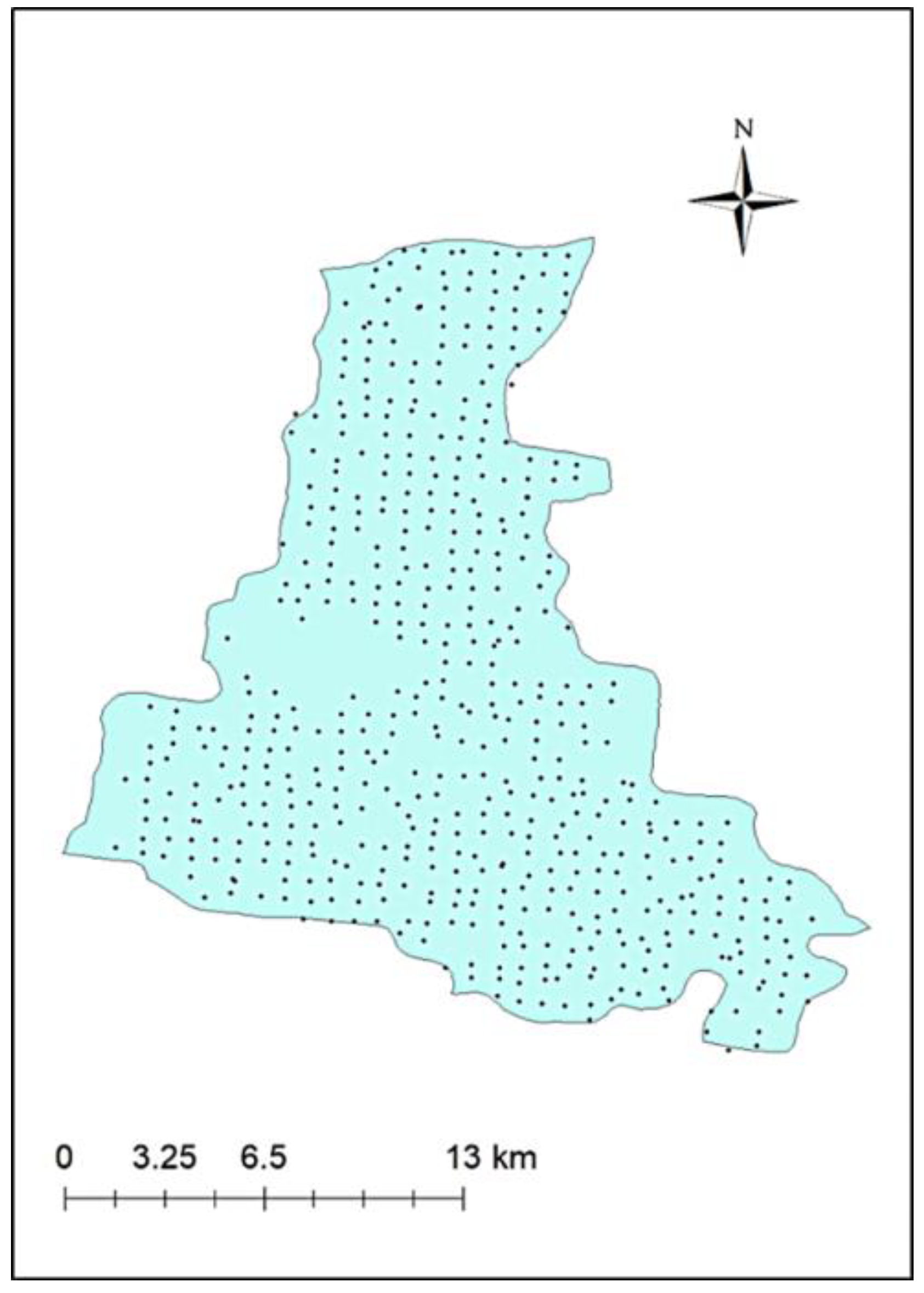
2.1. Study Area and Soil Sampling

The 1 km×1 km grid survey was used to collect soil samples in Quzhou County, Hebei Province, China, which covers about 667 km². The average annual temperature and precipitation in the study region are approximately 13.1 °C and 556 mm, respectively. The soil type is mainly Fluvo-aquic soil. Five hundred and ten topsoil (0–20 cm) samples were obtained using a soil auger. The detailed position information of the sampling sites was designed and recorded using a hand-held GNSS device (Figure 1).

2.2. Spectral Measurement and SOM and TN Content Analysis

The obtained soil samples were air-dried at room temperature and crushed before being passed through a 2 mm mesh sieve to remove any plant roots and debris prior to analysis. Each soil sample was divided into two portions: one for spectral measurement and the other for SOM and soil TN content analysis. The soil samples to be used for MIR analysis were finely ground, passed through a 0.15 mm (100–mesh) sieve [43,44], dried in oven at 105 °C for 2 h, and then stored in a desiccator (Nalgene, Thermo Fisher, Waltham, MA, USA) until they were ready to be scanned. SOM was chemically determined using a potassium dichromate oxidation colorimetry [45], with values ranging from 3.20 g/kg to 32.70 g/kg (

Table 1. SOM and TN statistical characteristics of soil samples in Quzhou County.

Soil Property	Mean	Median	SD	Minimum	Maximum
SOM (g/kg)	13.80	13.90	0.36	3.20	32.70
TN (g/kg)	0.96	0.96	0.26	0.21	2.43

Note: SD: standard deviation.

). Soil TN content was determined by the semi-micro automated Kjeldahl method [46], with values ranging from 0.21 g/kg to 2.42 g/kg (Table 1).

Soil MIR diffuse reflectance spectra were collected using a Fourier transform infrared spectrometer (FT-IR) Tensor II with an HTS-XT high-throughput diffuse reflectance accessory (Bruker Optics, Karlsruhe, Germany). The spectrometer was equipped with a mercury cadmium telluride detector cooled by liquid nitrogen. The measured wavebands ranged from 4000 to 600 cm⁻¹ with a resolution of 4 cm⁻¹. Soil samples were loaded into 24-well spot aluminum microtiter plates. Prior to each scan, the sensor was calibrated using the background spectrum of the reference plate. Gold background measurements of the first well were taken before each single measurement to account for changes in temperature and air humidity. Soil samples were loaded into two replicate wells, each scanned 32 times, and the two spectra were averaged to account for within-sample variability and differences in packing density and particle size.

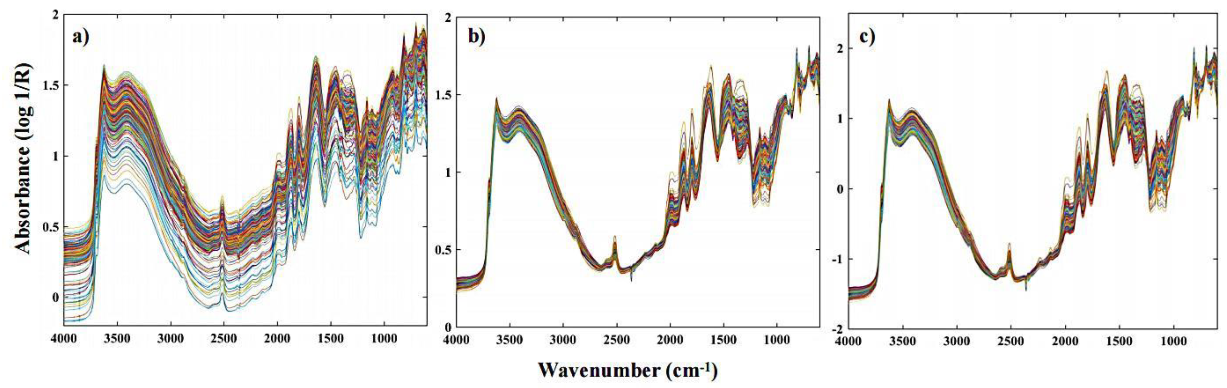
2.3. Spectral Pre-Processing

Original soil MIR spectra and spectra after pre-processing are shown in Figure 2. Spectral pre-processing with multiplicative scatter correction (MSC) [47] was carried out for SOM, and spectra pre-processed by MSC are shown in Figure 2b. For TN, spectral pre-processing was completed using a standard normalized variate (SNV) [48], and pre-processed spectra by SNV are shown in Figure 2c.

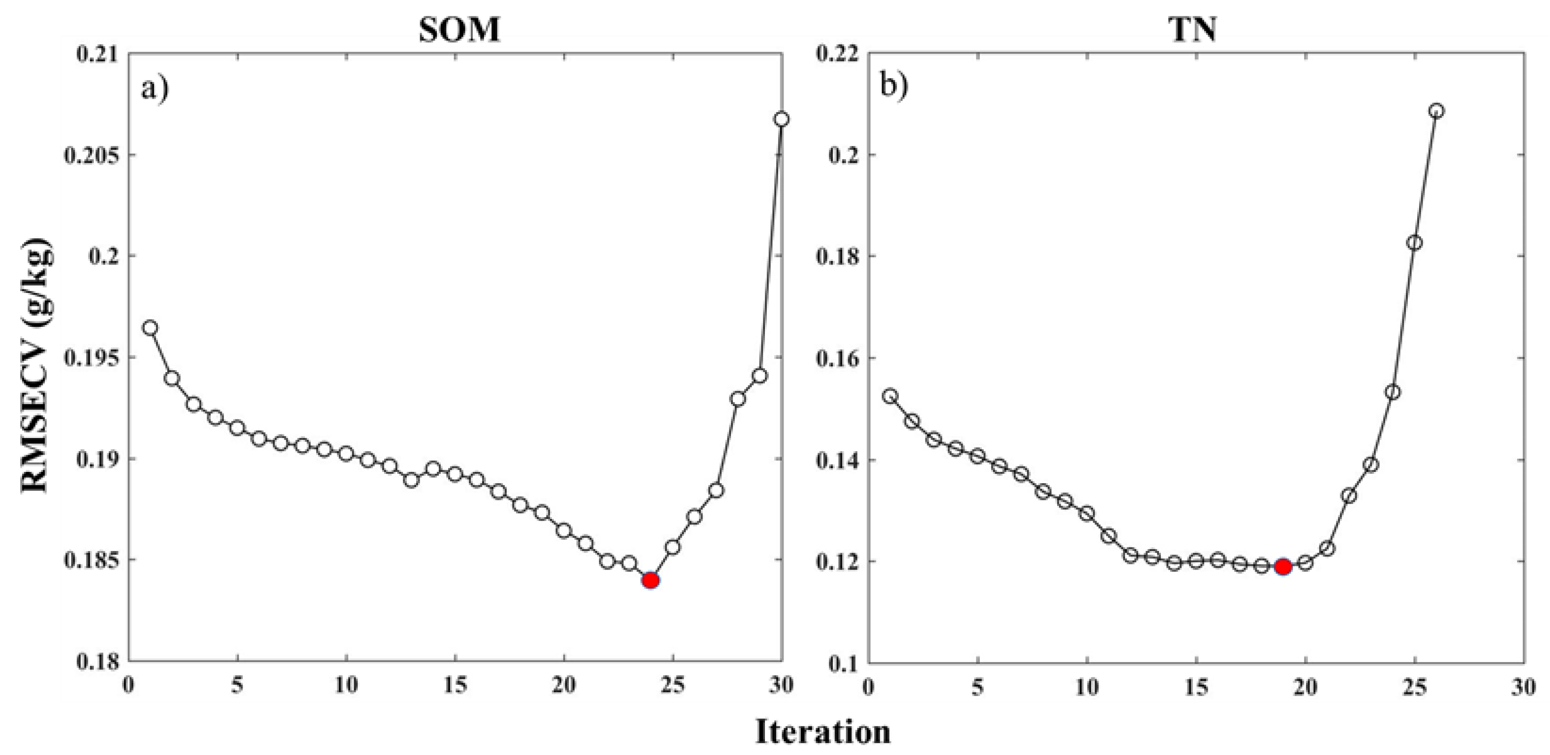
2.4. Variable Selection Methods

2.4.1. Stability Competitive Adaptive Reweighting Algorithm (sCARS)

sCARS mainly relies on the stability of the selected variables, so it also improves the stability of variable selection while continuing CARS′s operation of screening variables [35].

The steps involved in the sCARS algorithm operation is as follows [34]:

Step 1: Compute the stability of each wavenumber variable.

Step 2: On the basis of the exponentially decreasing function (EDF) and adaptive reweighted sampling (ARS) method, a subset of variables with strong stability is selected.

Step 3: Repeat the first step and the second step, and finally obtain K subsets of variables, and use the selected subsets of variables to establish a PLSR model, in which the subset of variables with the lowest root-mean-squared error of cross-validation (RMSECV) is the best characteristic variable.

The algorithm procedure can be illustrated in a flow chart of Figure 3 [34].

The following parameters were used in the research: Monte Carlo sampling (MCS) number M = 500, MCS sampling ratio r = 0.7, and calculation loops number N = 100. The processes of the sCARS algorithm were conducted using MATLAB R2020b.

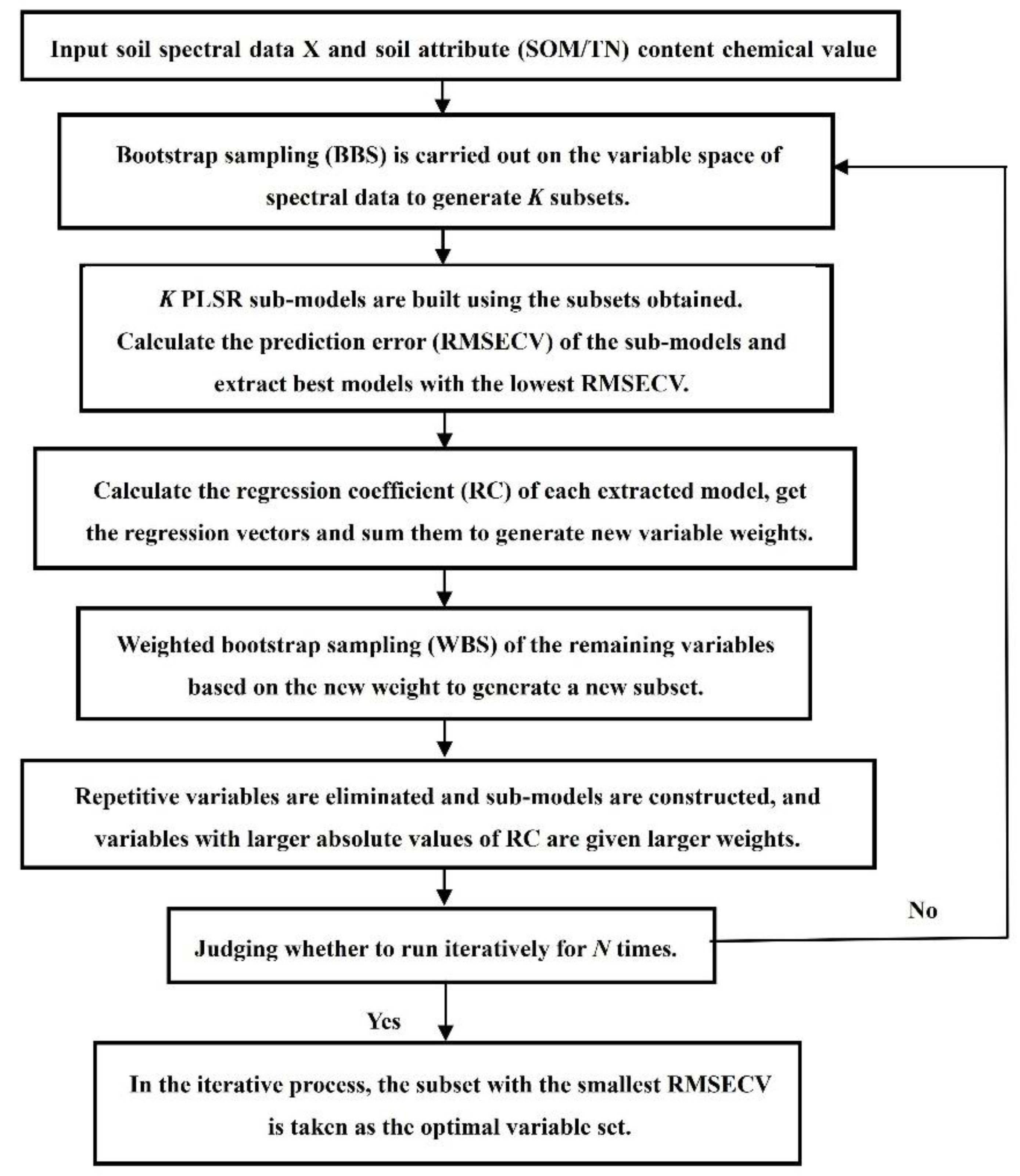
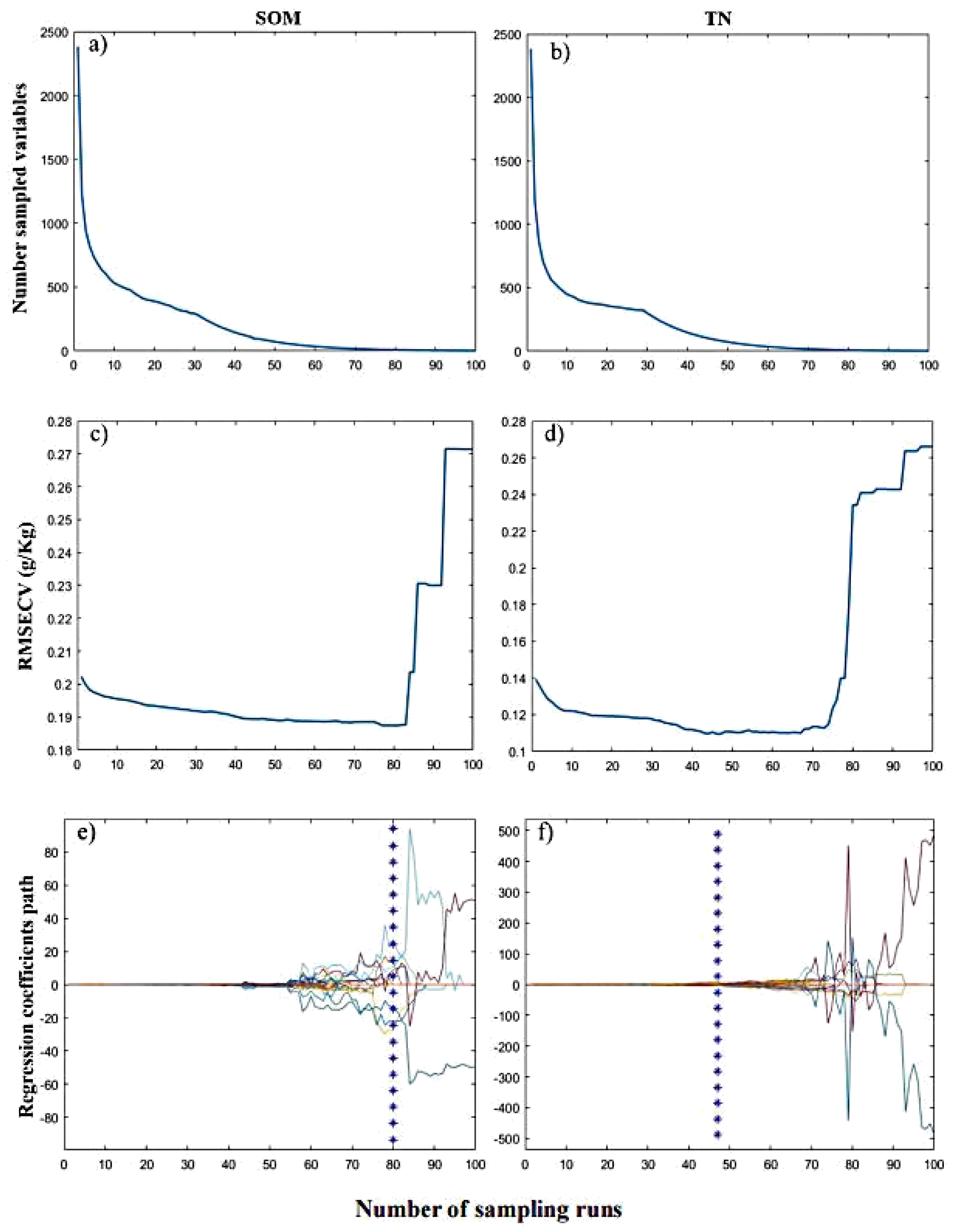
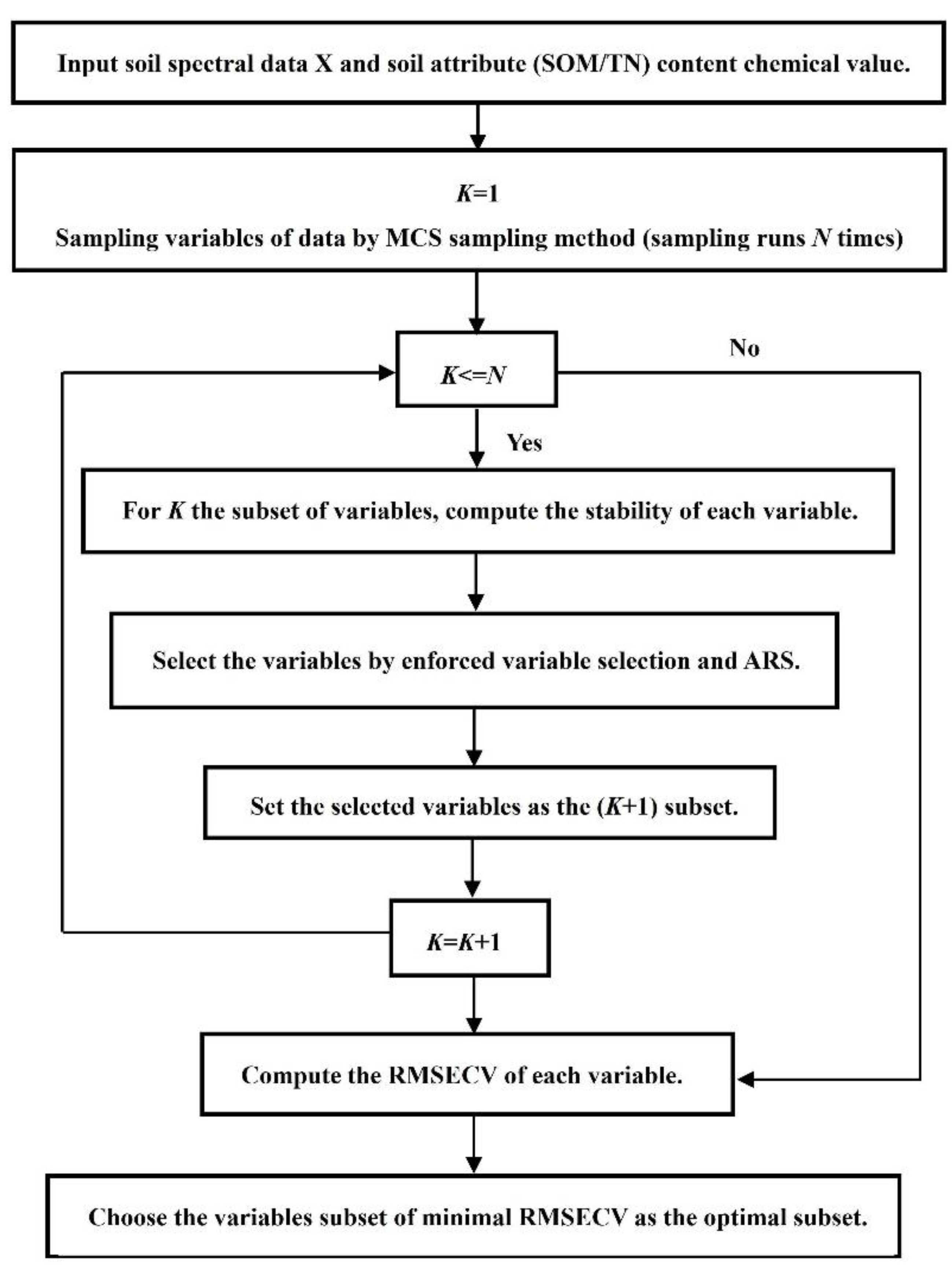
2.4.2. Bootstrapping Soft Shrinkage (BOSS)

BOSS uses a strategy called a soft-shrinking strategy in variable selection. The soft-shrinking strategy assigns smaller weights to the less informative variables, while the hard-shrinking strategy directly eliminates the less informative variables [30]. Thus, these variables still have the chance to participate in the models. The advantage of the soft-shrinking strategy is that it can reduce the risk of eliminating important variables in the optimization process and can choose a combination of variables with better prediction ability [36].

The main process of the BOSS algorithm operation is as follows [36]:

Suppose there is a matrix X_N×P which contains N samples and P variables. The prediction attribute vector is y_N×1.

Step 1: Apply bootstrap sampling (BSS) in variable space to generate K subsets. In this process, each variable has the same probability to be selected into subsets.

Step 2: K PLSR sub-models are established by using the obtained subsets. Additionally, the RMSECV of the sub-model is calculated, and the lowest RMSECV is the best model.

Step 3: Calculate the regression coefficient (RC) of the extracted model. The absolute values of the elements in each regression vector are normalized, and the normalized regression vectors are summed to obtain the new weights of variables.

Step 4: Weighted bootstrap sampling (WBS) is used to generate new subsets of variables and extract unique variables to establish sub-models. Repeat Step 2 to Step 4 until the number of variables in the new subset is 1, and the subset with the lowest RMSECV is taken as the optimal variable set during calculation.

The algorithm procedure can be illustrated in a flow chart of Figure 4.

The following parameters were used in the research: the maximal number of latent variables for cross-validation = 5; fold = 5; pretreatment method = center; the number of bootstraps = 1000; speed = 0 [30,36]. The whole process of the BOSS method was conducted in MATLAB R2020b with the BOSS toolbox, available at: http://www.mathworks.com/matlabcentral/fileexchange/52770-boss (accessed on 16 September 2021).

2.5. Model Calibration

The whole dataset was divided into a calibration dataset (n = 357) and a validation dataset (n = 135) using the Kennard–Stone algorithm [49]. Two multivariate methods (PLSR and MLR) were used for model calibration.

PLSR is similar to principal component regression, as both employ statistical rotations to overcome the problems of high dimensionality and multicollinearity [23]. This method selected continuous orthogonal factors to maximize the covariance between prediction variables and response variables [33]. Additional details of PLSR have been described by Viscarra Rossel and Behrens (2010) [40].

MLR analysis is also the most basic and simplest in multivariate regression analysis, and the mathematical formula expressing this quantitative relationship is called the multivariate linear regression model. Under the condition of studying linear correlation, linear regression can be divided into two types: one is an independent variable and a dependent variable, and the relationship between them can be approximated using a straight line. This regression analysis is called unary linear regression. The other is the multiple linear regression analysis in the case of two or more independent variables versus one dependent variable [50]. In fact, when studying problems, a phenomenon is often associated with multiple factors. It is more effective and more realistic to predict or estimate the dependent variable using the optimal combination of multiple independent variables. Therefore, multivariate linear regression is more effective than univariate linear regression. In the process of applying a regression model, only the same model and data can be used, and the unique result can be calculated using a standard statistical method, which ensures the accuracy and stability of the result. MLR is a modeling technique commonly used in spectral prediction that usually gives relatively good prediction accuracy [40,41].

2.6. Model Evaluation

To assess the goodness of fit of the predictive models and their performance against independent validation sets, we used the coefficient determination of prediction (R_p²) (Equation (1)), the root-mean-square error of prediction (RMSEp) (Equation (2)), and the residual prediction deviation of prediction (RPD) (Equation (3)). R² represents the degree to which the dependent variable is fully interpreted. The RMSE measures the accuracy of predictions, being an easily interpreted statistic because it has the same data units. The RPD is the ratio of the standard deviation of the measured values to the RMSEp, and it was used to define the quality of the derived models [51]. These evaluation parameters could be specifically defined by the following formulae:

$${R_P}^2=1-\frac{{{\displaystyle \sum }}_{i=1}^n{(y_i-{\hat{y}}_i)}^2}{{{\displaystyle \sum }}_{i=1}^n{(y_i-{\overline{y}}_i)}^2}$$

(1)

$$RMSEp=\sqrt{\frac{1}{n}{\displaystyle \sum }_{i=1}^n{(y_i-{\widehat{y}}_i)}^2}$$

(2)

$$RPD=\frac{SD}{RMSEP}$$

(3)

where y_i and ${\widehat{y}}_i$ refer to the measured value and the corresponding estimated value, respectively, ${\overline{y}}_i$ is the average of the estimated values, n denotes the number of samples, and SD is the standard deviation of the measured values.

In soil science, the RPD was used as a classifier of prediction results in the common scheme defined by Chang et al. (2001). When RPD > 2.0, the estimation model was more reliable. Values of RPD between 1.4 and 2.0 suggest that the predictive power could be improved, and RPD < 1.4 indicates that the model failed to predict the soil properties (i.e., it had no prediction capability) [52].

3. Results

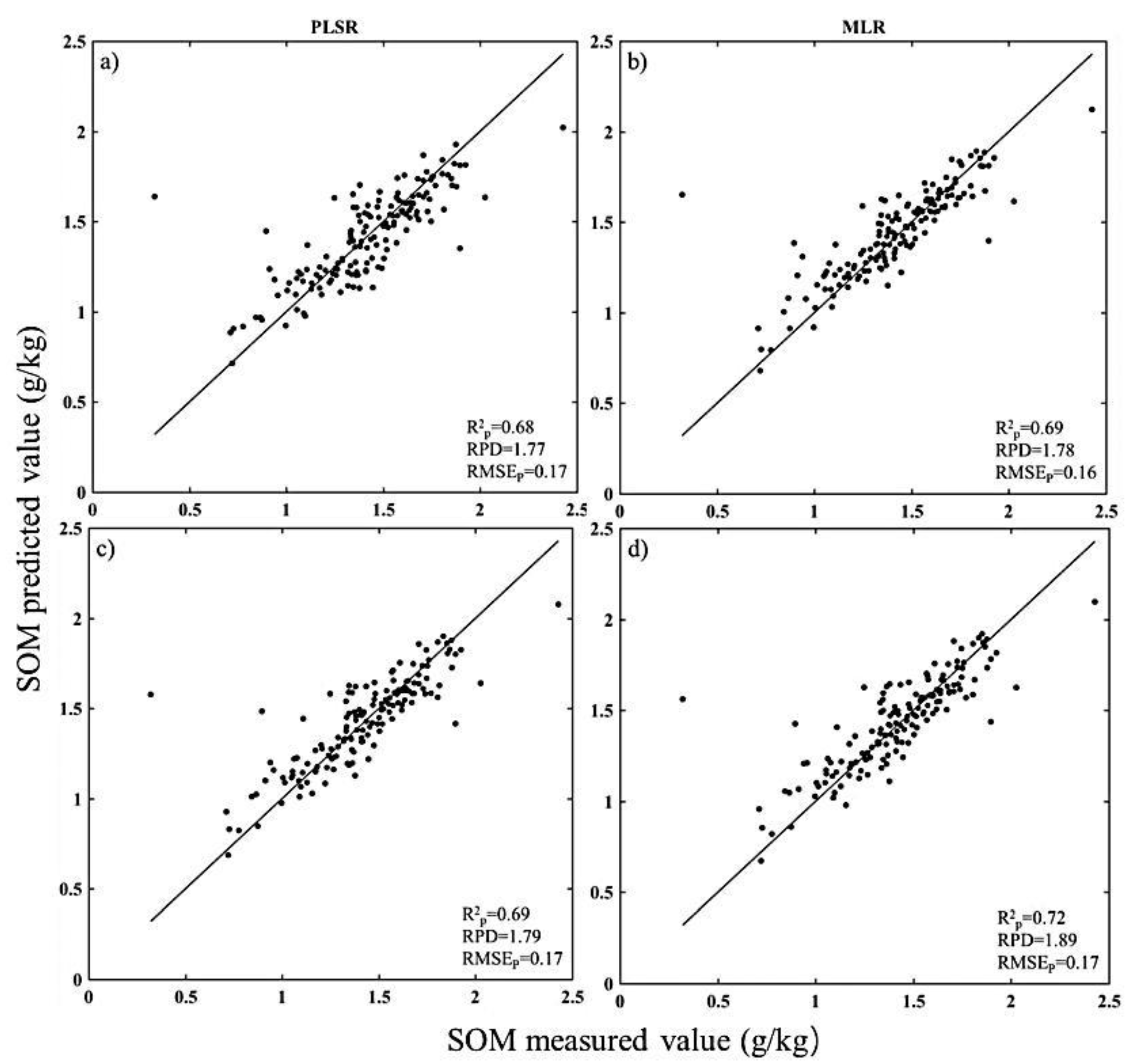
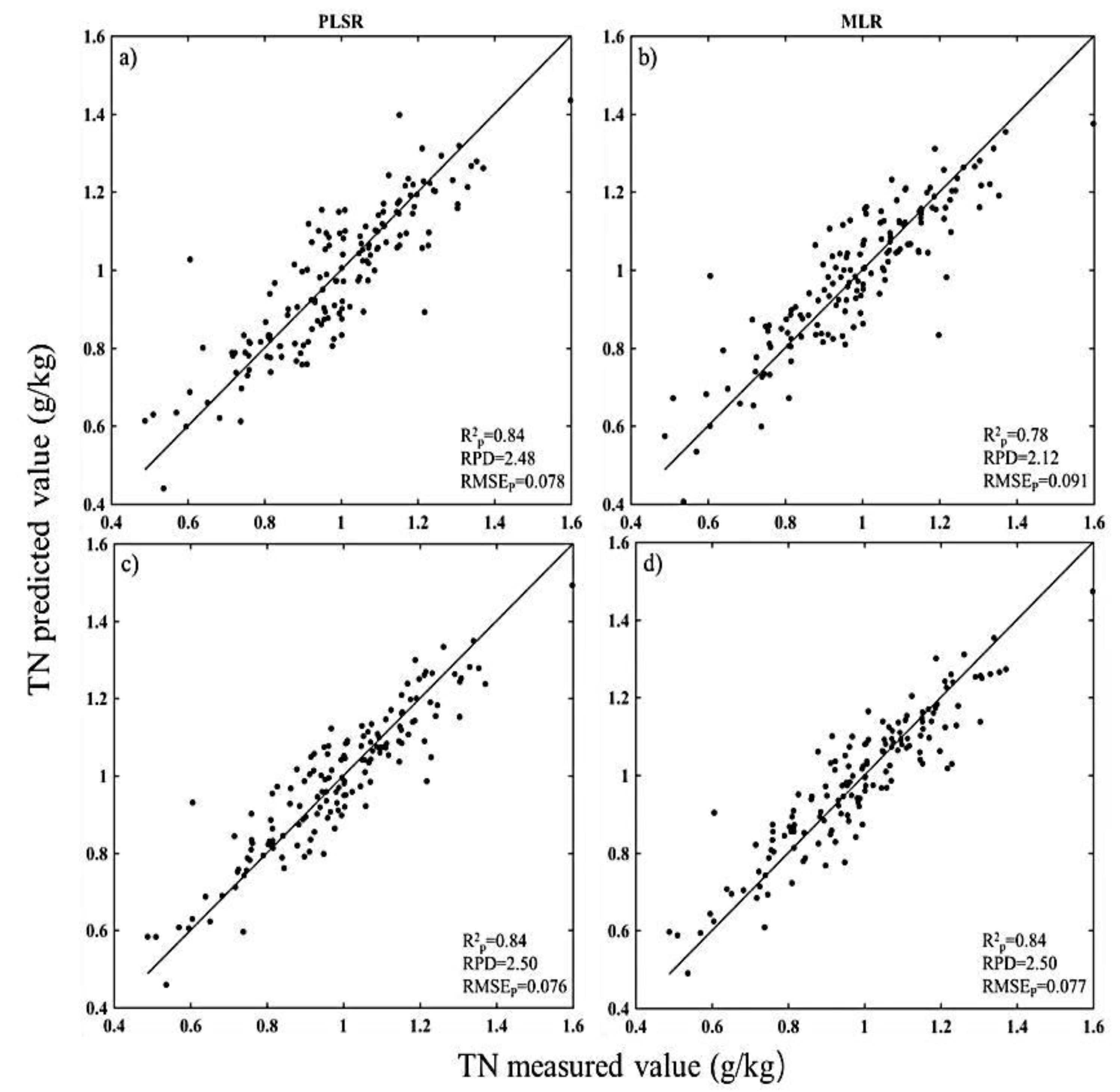
3.1. Estimation Accuracies and Model Parsimony

The performances of different variable selection models are illustrated in

Table 2. Modeling results of SOM and TN screened with different variables selection methods.

Soil Property	Model	Variable Number	Time (min)	Validation Set
				RP2	RPDp	RMSEP (g/kg)
SOM	None-PLSR	2382	2	0.68	1.77	0.17
	BOSS-PLSR	14	200	0.68	1.77	0.17
	BOSS-MLR	14	3	0.69	1.78	0.16
	sCARS-PLSR	31	20	0.69	1.79	0.17
	sCARS-MLR	31	3	0.72	1.89	0.10
TN	None-PLSR	2382	2	0.81	2.29	0.084
	BOSS-PLSR	44	240	0.84	2.48	0.078
	BOSS-MLR	44	3	0.78	2.12	0.091
	sCARS-PLSR	27	20	0.84	2.50	0.076
	sCARS-MLR	27	3	0.84	2.50	0.077

. All estimation models of SOM have a similar prediction accuracy with 0.65 < R_p² < 0.75 and 1.4 < RPD < 2.0 (satisfactory predictions), while R_p² and RPD values in all estimation models of TN are greater than 0.75 or 2.0 (good predictions). The R_p² and RPD of SOM estimation models based on the BOSS and sCARS variables selection methods were equal to or higher than that of the full MIR spectrum model. BOSS selected 14 variables (out of 2382 spectral variables), whereas sCARS selected 31 variables (Table 2).

For TN, the PLSR models developed with selected wavenumbers gave better estimations compared to the models developed with the full spectrum. BOSS selected 44 variables (accounting for 1.85% of all variables), while sCARS selected 27 variables (accounting for 1.13% of all variables) to be input in the model calibration. The results illustrated that BOSS and sCARS were highly efficient approaches for extracting informative wavenumbers and mitigating redundant wavenumbers. The MLR model combined with the sCARS method yielded the most accurate estimation result for SOM (R_p² = 0.72 and RPD = 1.89). For TN, the best performing result was obtained by the sCARS-MLR model (R_p² = 0.84 and RPD = 2.50) and sCARS-PLSR model (R_p² = 0.84 and RPD = 2.50), followed by the BOSS-PLSR model (R_p² = 0.84 and RPD = 2.48) and BOSS-MLR model (R_p² = 0.78 and RPD = 2.12).

The BOSS algorithm, due to its instability, needs to run 50 times, which usually takes several hours. On the contrary, the sCARS algorithm runs only once since it is stable, taking usually less than an hour. Hence, due to the long computation time of BOSS, one alternative was to use the sCARS method, which is in agreement with another study [35].

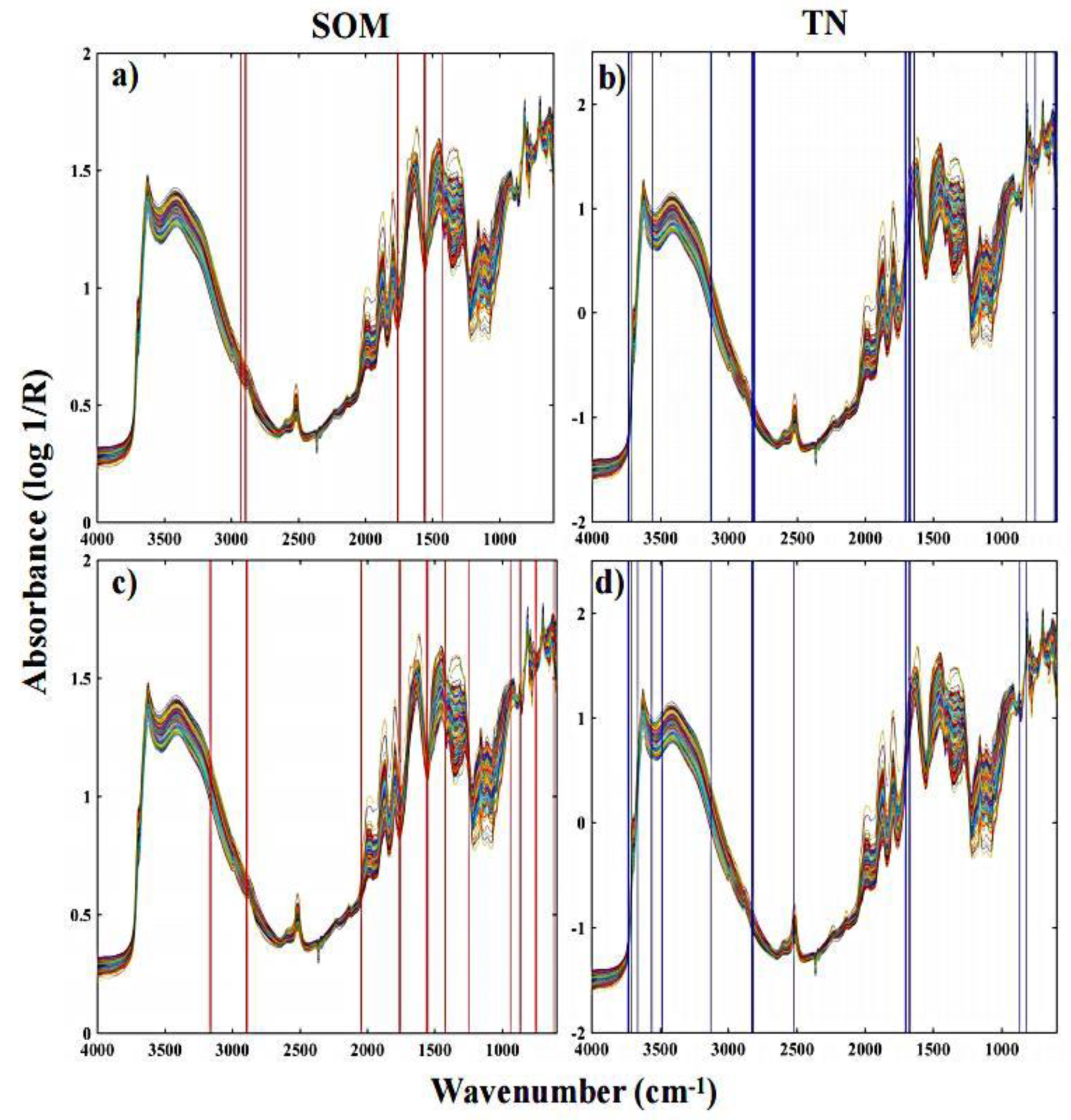
3.2. Key Wavenumbers

In the BOSS algorithm, sub-models are generated according to the weights of variables. The weights of variables are obtained based on the RC of sub-models. Each sub-model corresponds to a random combination of variables, in which the variables with larger weights have larger probabilities to participate. Five-fold cross-validation is applied to explore its predictability. The evolution of RMSECV (g/kg) in sub-models in each iteration of the BOSS algorithm is displayed in Figure 5. For SOM, the RMSECV reached the minimum value (0.18 g/kg) when the number of sampling runs was equal to 24 (Figure 5a). Fourteen spectral wavenumber variables were selected out of 2382 spectral variables for SOM, which was 0.58% of the number of the full spectrum. For TN, the RMSECV reached the minimum value (0.12 g/kg) when the number of sampling runs was equal to 19 (Figure 5b). Forty-four spectral wavenumber variables were selected out of 2382 spectral variables for TN, which is 1.85% of the number of the full spectrum. The final selected spectral variables for SOM and TN are illustrated in Figure 6a in the red region and Figure 6b in the blue region, respectively.

Figure 7 shows the variable selection process using sCARS method. The number of sampling variables of SOM and TN decreased with the increasing number of sampling runs (Figure 7a,b). Figure 7c,d presents the changing trend of 10-fold RMSECV values with the increasing number of sampling runs. The RMSECV reached the minimum value (0.19 g/kg for SOM and 0.11 g/kg for TN) when the number of sampling runs was equal to 80 and 48 for SOM and TN, respectively. Figure 7e,f illustrates the variation trend of the regression coefficient path for different sampling runs. The optimal subset corresponded to the lowest RMSECV, marked by a vertical line with asterisks. Accordingly, 31 and 27 spectral variables of SOM and TN were selected by sCARS in MIR spectrum, which accounted for 1.30% and 1.13% of the full spectrum (Figure 6c,d).

The final effective wavenumber variables selected by BOSS and sCARS for estimating SOM and TN content are shown in Figure 6 and

Table 3. Key wavenumbers (MIR) identified from the BOSS and sCARS runs.

Soil Property	Variable Selection Method	Variable Number	Characteristic Variable (cm−1)
SOM	BOSS	14	2930,2928, 2894, 2893, 2891, 2890, 1760–1755, 1563, 1555, 1554, 1427
	sCARS	31	3168, 3156, 2894–2888, 2045–2043, 1761–1755, 1561, 1560, 1555–1551, 1422, 1421, 1247, 938, 867–864, 754, 745, 617
TN	BOSS	44	3736, 3733, 3728, 3707, 3560, 3130–3126, 2827–2818, 2810, 2808, 1707, 1705–1700, 1698, 1678–1665, 1641–1638, 817, 754, 617, 605, 604
	sCARS	27	3733, 3728, 3727, 3707, 3661, 3560, 3558, 3484, 3483, 3127, 2825–2818, 2518, 1704–1700, 1675–1671, 867, 817

. Keys were found in the X−H stretching (C-H, N-H, and O-H groups containing hydrogen) region from 4000 to 2500 cm⁻¹, in the triple- and double-bond regions from 2500 to 1500 cm⁻¹, and in the fingerprint MIR region from 1500 to 600 cm⁻¹. Then, 2894–2890 cm⁻¹, 1760–1755 cm⁻¹, 1563 cm⁻¹, 1555 cm⁻¹, and 1554 cm⁻¹ were determined individually to be the sensitive wavenumbers of SOM content (Figure 6a,c), and 3733 cm⁻¹, 3728 cm⁻¹, 3707 cm⁻¹, 3560 cm⁻¹, 3127 cm⁻¹, 2825–2818 cm⁻¹, 1704–1700 cm⁻¹, 1675 cm⁻¹, 1673 cm⁻¹, 1671 cm⁻¹, and 817 cm⁻¹ were determined individually to be the sensitive wavenumbers of soil TN content (Figure 6b,d).

4. Discussion

Important SOM features are located at 1740–1698 cm⁻¹ (C=O groups in carboxylic acids, aldehydes, and ketones), 1640–1600 cm⁻¹ (amide I band (C-O, C-N) of proteins, C=O of carboxylic acids and ketones), and 1575–1400 cm⁻¹ (amide II band, N-H) [23]. The intensity of the region 1740–1698 cm⁻¹ can be used as a measure of hydrophilic organic components [53] and was identified as a key region for soil TN [38]. Key wavenumbers of TN in MIR identified from the CARS-PLSR runs were 1676–1672 cm⁻¹, 1260 cm⁻¹, and 1036 cm⁻¹ [23]. The report is consistent with the characteristic variables selected in the present study.

BOSS is a strategy that combines MPA and WBS. The absolute value of RC is the criteria of variables. The advantage of MPA is that it considers the combined effect between variables. WBS reduces the effect of collinearity [36]. BOSS focuses more on using the information in the model RC. Yan et al. (2019) reported that BOSS selected fewer variables, gave lower a RMSEP value, and better predicted the starch content of corn using NIR spectra compared to other methods, including Monte Carlo uninformative variables elimination (MCUVE), GA, and CARS [35]. Moreover, Lao et al. (2021) reported that BOSS-ELM (Extreme Learning Machine) models outperformed MCUVE-ELM models in estimating the contents of soil salt and soluble ions using Vis-NIR spectroscopy [30].

The sCARS method enhances the stability of variable selection by using variable stability as a variable selection indicator and continues the variable selection process of the CARS method with fast calculation speed. When Yan et al. (2019) employed sCARS and MCUVE to predict the real extract concentration of beer in NIR spectroscopy, the authors reported that both methods had comparative performance; however, MCUVE retained fifteen times more variables than sCARS did [35]. The sCARS method was also employed to extract the characteristic bands of SOM via Vis-NIR spectroscopy, and 51 variables were selected (out of 2000 spectral variables). Compared to modeling based on the full bands, the combination of variable selection and regression methods could effectively improve the modeling efficiency while ensuring the accuracy of the model [54].

The variable selection algorithm combines the prediction model, and the scatter diagrams of PLSR and MLR, respectively, are displayed in Figure 8 and Figure 9. The solid black line in each plot represents the 1:1 line. As shown in the figures, the measured value and predicted value of SOM and TN content in the MLR models were generally closer to the 1:1 line compared to the PLSR models. MLR is used to substitute independent variables into the regression equation in turn, and eliminate irrelevant or insignificant independent variables according to the score and the contribution rate of independent variables to dependent variables so as to obtain an accurate and stable prediction model [55]. Jia et al. (2014) used MCUVE and SPA combined with PLSR and MLR for the prediction of soil nitrogen and organic carbon using NIR diffuse reflectance spectroscopy [56]. They reported that although the application of the SPA-MLR method did not lead to satisfactory predictions, the variable number was much reduced and the calibration models were simplified, which made it possible to use a cheap and simple spectrometer for the measurement of soil nitrogen.

5. Conclusions

In this study, two variable selection techniques (i.e., sCARS and BOSS) were employed to circumvent the problem of multicollinearity in MLR to improve the estimation accuracy of SOM and TN models developed with DRIFT-MIR spectra. The results showed that by using a few selected wavenumbers, BOSS and sCARS can give even better predictive performance in much less computation time when compared with the full spectrum model. The MLR model combined with the sCARS method yielded the most accurate estimation result for SOM and TN. The results of the present study indicated that MLR with sCARS could decrease the computation complexity and simplify the model, and consequently improve the prediction ability. Thus, using DRIFT-MIR spectroscopy together with MLR and sCARS is a good alternative for estimating the SOM and TN of soils.

References

1. Ahmadi, A.; Emami, M.; Daccache, A.; He, L.Y. Soil properties prediction for precision agriculture using visible and near-infrared spectroscopy: A systematic review and Meta-analysis. Agronomy 2021, 11, 433. [Google Scholar] [CrossRef]
2. Reda, R.; Saffaj, T.; Ilham, B.; Saidi, O.; Issam, K.; Brahim, L.; El Hadrami, E.M. A comparative study between a new method and other machine learning algorithms for soil organic carbon and total nitrogen prediction using near infrared spectroscopy. Chemometr. Intell. Lab. Syst. 2019, 195, 103873. [Google Scholar] [CrossRef]
3. Gebbers, R.; Adamchuk, V.I. Precision Agriculture and Food Security. Science 2010, 327, 828–831. [Google Scholar] [CrossRef]
4. Xu, D.; Zhao, R.; Li, S.; Chen, S.; Jiang, Q.; Zhou, L.; Shi, Z. Multi-sensor fusion for the determination of several soil properties in the Yangtze River Delta, China. Eur. J. Soil Sci. 2019, 70, 162–173. [Google Scholar] [CrossRef] [Green Version]
5. Reeves, J.B. Near- versus mid-infrared diffuse reflectance spectroscopy for soil analysis emphasizing carbon and laboratory versus on-site analysis: Where are we and what needs to be done? Geoderma 2010, 158, 3–14. [Google Scholar] [CrossRef]
6. Bellon-Maurel, V.; Mcbratney, A. Near-infrared (NIR) and mid-infrared (MIR) spectroscopic techniques for assessing the amount of carbon stock in soils-Critical review and research perspectives. Soil Biol. Biochem. 2011, 43, 1398–1410. [Google Scholar] [CrossRef]
7. Soriano-Disla, J.M.; Janik, L.J.; Viscarra, R.; Macdonald, L.M.; McLaughlin, M.J. The performance of visible, near-, and mid-infrared reflectance spectroscopy for prediction of soil physical, chemical, and biological properties. Appl. Spectrosc. Rev. 2014, 49, 139–186. [Google Scholar] [CrossRef]
8. Barra, I.; Haefele, S.M.; Sakrabani, R.; Kebede, F. Soil spectroscopy with the use of chemometrics, machine learning and pre-processing techniques in soil diagnosis: Recent advances—A review. TrAC Trends Anal. Chem. 2021, 135, 116166. [Google Scholar] [CrossRef]
9. Guo, P.; Li, T.; Gao, H.; Chen, X.W.; Cui, Y.F.; Huang, Y.R. Evaluating calibration and spectral variable selection methods for predicting three soil nutrients using Vis-NIR spectroscopy. Remote Sens. 2021, 13, 4000. [Google Scholar] [CrossRef]
10. Lazaar, A.; Mouazen, A.M.; EL Hammouti, K.; Fullen, M.; Pradhan, B.; Memon, M.S.; Andich, K.; Monir, A. The application of proximal visible and near-infrared spectroscopy to estimate soil organic matter on the Triffa Plain of Morocco. Int. Soil Water Conserv. Res. 2020, 8, 195–204. [Google Scholar] [CrossRef]
11. de Santana, F.B.; de Souza, A.M.; Poppi, R.J. Green methodology for soil organic matter analysis using a national near infrared spectral library in tandem with learning machine. Sci. Total Environ. 2019, 658, 895–900. [Google Scholar] [CrossRef] [PubMed]
12. Terra, F.S.; Dematte, J.A.M.; Viscarra Rossel, R.A. Spectral libraries for quantitative analyses of tropical Brazilian soils: Comparing vis–NIR and mid-IR reflectance data. Geoderma 2015, 255, 81–93. [Google Scholar] [CrossRef]
13. Ji, W.J.; Li, S.; Chen, S.C.; Shi, Z.; Viscarra Rossel, R.A.; Mouazen, A.M. Prediction of soil attributes using the Chinese soil spectral library and standardized spectra recorded at field conditions. Soil Till. Res. 2016, 155, 492–500. [Google Scholar] [CrossRef]
14. Xu, S.X.; Zhao, Y.C.; Wang, M.Y.; Shi, X.Z. Comparison of multivariate methods for estimating selected soil properties from intact soil cores of paddy fields by Vis–NIR spectroscopy. Geoderma 2018, 310, 29–43. [Google Scholar] [CrossRef]
15. Morellos, A.; Pantazi, X.E.; Moshou, D.; Alexandridis, T.; Whetton, R.; Tziotzios, G.; Wiebensohn, J.; Bill, R.; Mouazen, A.M. Machine learning based prediction of soil total nitrogen, organic carbon and moisture content by using VIS-NIR spectroscopy. Biosyst. Eng. 2016, 152, 104–116. [Google Scholar] [CrossRef] [Green Version]
16. Conforti, M.2; Matteucci, G.; Buttafuoco, G. Using laboratory Vis-NIR spectroscopy for monitoring some forest soil properties. J. Soils Sediments 2018, 18, 1009–1019. [Google Scholar] [CrossRef]
17. Askari, M.S.; O’Rourke, S.M.; Holden, N.M. Evaluation of soil quality for agricultural production using visible-near-infrared spectroscopy. Geoderma 2015, 243, 80–91. [Google Scholar] [CrossRef]
18. Tümsavaş, Z. Application of visible and near infrared reflectance spectroscopy to predict total nitrogen in soil. J. Environ. Biol. 2017, 38, 1101–1106. [Google Scholar] [CrossRef]
19. Zhang, Y.; Li, M.Z.; Zheng, L.H.; Qin, Q.M.; Lee, W.S. Spectral features extraction for estimation of soil total nitrogen content based on modified ant colony optimization algorithm. Geoderma 2019, 333, 23–34. [Google Scholar] [CrossRef]
20. McCarty, G.W.; Reeves III, J.B.; Reeves, V.B.; Follett, R.F.; Kimble, J.M. Mid-infrared and near-infrared diffuse reflectance spectroscopy for soil carbon management. Soil Sci. Soc. Am. J. 2002, 66, 640–646. [Google Scholar] [CrossRef]
21. McCarty, G.W.; Reeves, J.B., III. Comparison of near infrared and mid infrared diffuse reflectance spectroscopy for field-scale measurement of soil fertility parameters. Soil Sci. 2006, 171, 94–102. [Google Scholar] [CrossRef] [Green Version]
22. Xie, H.T.; Yang, X.M.; Drury, C.F.; Yang, J.Y.; Zhang, X.D. Predicting soil organic carbon and total nitrogen using mid- and near-infrared spectra for Brookston clay loam soil in Southwestern Ontario, Canada. Can. J Soil Sci. 2011, 91, 53–63. [Google Scholar] [CrossRef]
23. Vohland, M.; Ludwig, M.; Thiele-Bruhn, S.; Ludwig, B. Determination of soil properties with visible to near- and mid-infrared spectroscopy: Effects of spectral variable selection. Geoderma 2014, 223–225, 88–96. [Google Scholar] [CrossRef]
24. Knox, N.M.; Grunwald, S.; McDowell, M.L.; Bruland, G.L.; Myers, D.B. Harris W G. Modelling soil carbon fractions with visible near-infrared (VNIR) and mid-infrared (MIR) spectroscopy. Geoderma 2015, 239–240, 229–239. [Google Scholar] [CrossRef]
25. Haghi, R.K.; Perez-Fernandez, E.; Robertson, A.H.J. Prediction of various soil properties for a national spatial dataset of Scottish soils based on four different chemometric approaches: A comparison of near infrared and mid-infrared spectroscopy. Geoderma 2021, 396, 115071. [Google Scholar] [CrossRef]
26. dos Santos, U.J.; de Melo Dematte, J.A.; Cezar Menezes, R.S.; Dotto, A.C.; Barbosa Guimaraes, C.C.; Rodrigues Alves, B.J.; Primo, D.C.; de Sa Barretto Sampaio, E.V. Predicting carbon and nitrogen by visible near-infrared (Vis-NIR) and mid-infrared (MIR) spectroscopy in soils of Northeast Brazil. Geoderma Reg. 2020, 23, e00333. [Google Scholar] [CrossRef]
27. Johnson, J.M.; Vandamme, E.; Senthilkumar, K.; Sila, A.; Shepherd, K.D.; Saito, K. Near-infrared, mid-infrared or combined diffuse reflectance spectroscopy for assessing soil fertility in rice fields in sub-Saharan Africa. Geoderma 2019, 354, 113840. [Google Scholar] [CrossRef]
28. Seybold, C.A.; Ferguson, R.; Wysocki, D.; Bailey, B.; Anderson, J.; Nester, B.; Schoeneberger, P.; Wills, S.; Libohova, Z.; Hoover, D.; et al. Application of Mid-Infrared Spectroscopy in Soil Survey. Soil Sci. Soc. Am. J. 2019, 83, 1746–1759. [Google Scholar] [CrossRef]
29. Xiong, Y.R.; Zhang, R.Q.; Zhang, F.Y.; Yang, W.Y.; Kang, Q.D.; Chen, W.C.; Du, Y.P. A spectra partition algorithm based on spectral clustering for interval variable selection. Infrared Phys. Technol. 2020, 105, 103259. [Google Scholar] [CrossRef]
30. Lao, C.C.; Chen, J.Y.; Zhang, Z.T.; Chen, Y.W.; Ma, Y.; Chen, H.R.; Gu, X.B.; Ning, J.F.; Jin, J.M.; Li, X.W. Predicting the contents of soil salt and major water-soluble ions with fractional-order derivative spectral indices and variable selection. Comput. Electron. Agric. 2021, 182, 106031. [Google Scholar] [CrossRef]
31. Kawamura, K.; Nishigaki, T.; Tsujimoto, Y.; Andriamananjara, A.; Rabenaribo, M.; Asai, H.; Rakotoson, T.; Razafimbelo, T. Exploring relevant wavelength regions for estimating soil total carbon contents of rice fields in Madagascar from Vis-NIR spectra with sequential application of backward interval PLS. Plant Prod. Sci. 2021, 24, 1–14. [Google Scholar] [CrossRef]
32. Vohland, M.; Ludwig, M.; Harbich, M.; Emmerling, C.; Thiele-Bruhn, S. Using variable selection and wavelets to exploit the full potential of visible-near infrared spectra for predicting soil properties. J. Near Infrared Spectrosc. 2016, 24, 255–269. [Google Scholar] [CrossRef]
33. Cheng, H.; Wang, J.; Du, Y.K. Combining multivariate method and spectral variable selection for soil total nitrogen estimation by Vis-NIR spectroscopy. Arch. Agron. Soil Sci. 2020, 67, 1665–1678. [Google Scholar] [CrossRef]
34. Zheng, K.Y.; Li, Q.Q.; Wang, J.J.; Geng, J.P.; Cao, P.; Sui, T.; Wang, X.; Du, Y.P. Stability competitive adaptive reweighted sampling (SCARS) and its applications to multivariate calibration of NIR spectra. Chemometr. Intell. Lab. Syst. 2012, 112, 48–54. [Google Scholar] [CrossRef]
35. Yan, H.; Song, X.Z.; Tian, K.D.; Gao, J.X.; Li, Q.Q.; Xiong, Y.M.; Min, S.G. A modification of the bootstrapping soft shrinkage approach for spectral variable selection in the issue of over-fitting, model accuracy and variable selection credibility. Spectrochim. Acta A Mol. Biomol. Spectrosc. 2019, 210, 362–371. [Google Scholar] [CrossRef]
36. Deng, B.C.; Yun, Y.H.; Cao, D.S.; Yin, Y.L.; Wang, W.T.; Lu, H.M.; Luo, Q.Y.; Liang, Y.Z. A bootstrapping soft shrinkage approach for variable selection in chemical modeling. Anal. Chim. Acta 2016, 908, 63–74. [Google Scholar] [CrossRef]
37. Zhang, F.; Tang, X.J.; Tong, A.X.; Wang, B.; Wang, J.W. Bootstrapping soft shrinkage variable selection method based on the combination of frequency and regression coefficient. Chin. J. Sci. Instrum. 2020, 41, 64–70. [Google Scholar]
38. Hutengs, C.; Ludwig, B.; Jung, A.; Eisele, A.; Vohland, M. Comparison of portable and bench-top spectrometers for mid-infrared diffuse reflectance measurements of soils. Sensors 2018, 18, 993. [Google Scholar] [CrossRef] [PubMed] [Green Version]
39. Terhoeven-Urselmans, T.; Vagen, T.G.; Spaargaren, O.; Shepherd, K.D. Prediction of soil fertility properties from a globally distributed soil mid-Infrared spectral library. Soil Sci. Soc. Am. J. 2010, 74, 1792–1799. [Google Scholar] [CrossRef] [Green Version]
40. Viscarra Rossel, R.A.; Behrens, T. Using data mining to model and interpret soil diffuse reflectance spectra. Geoderma 2010, 158, 46–54. [Google Scholar] [CrossRef]
41. Al Maliki, A.; Bruce, D.; Owens, G. Prediction of lead concentration in soil using reflectance spectroscopy. Environ. Sci. Technol. 2014, 1–2, 8–15. [Google Scholar] [CrossRef]
42. Deiss, L.; Margenot, A.J.; Culman, S.W.; Demyan, M.S. Tuning support vector machines regression models improves prediction accuracy of soil properties in MIR spectroscopy. Geoderma 2020, 365, 114227. [Google Scholar] [CrossRef]
43. Le Guillou, F.; Wetterlind, W.; Rossel, R.A.V.; Hicks, W.; Grundy, M.; Tuomi, S. How does grinding affect the mid-infrared spectra of soil and their multivariate calibrations to texture and organic carbon? Soil Res. 2015, 53, 913–921. [Google Scholar] [CrossRef]
44. Janik, L.J.; Soriano-Disla, J.M.; Forrester, S.T.; McLaughlin, M.J. Effects of soil composition and preparation on the prediction of particle size distribution using mid-infrared spectroscopy and partial least-squares regression. Soil Res. 2016, 54, 889–904. [Google Scholar] [CrossRef]
45. Agricultural Chemistry Committee of China. Conventional Methods of Soil and Agricultural Chemistry Analysis; Science Press: Beijing, China, 1983. (In Chinese) [Google Scholar]
46. Nelson, D.; Sommers, L. Total nitrogen analysis of soil and plant tissues. JAOAC 1980, 63, 770–780. [Google Scholar] [CrossRef]
47. Wang, D.M.; Ji, J.M.; Gao, H.Z. The effect of MSC spectral pretreatment regions on near infrared spectroscopy calibration results. Spectrosc. Spectr. Anal. 2014, 34, 2387–2390. [Google Scholar]
48. Genkawa, T.; Shinzawa, H.; Kato, H.; Ishikawa, D.; Murayama, K.; Komiyama, M.; Ozaki, Y. Baseline correction of diffuse reflection near-infrared spectra using searching region standard normal variate (SRSNV). Appl. Spectrosc. 2015, 69, 1432–1441. [Google Scholar] [CrossRef]
49. Kennard, R.W.; Stone, L.A. Computer aided design of experiments. Technometrics 1969, 11, 137–148. [Google Scholar] [CrossRef]
50. Zou, H.M.; Li, X.C.; Shang, X.; Miao, C.H.; Huang, C.; Lu, J.H. Hyperspectral estimation of soil organic matter based on particle swarm optimization neural network. Sci. Surv. Mapp. 2019, 44, 146–150, 170. [Google Scholar]
51. Briedis, C.; Baldock, J.; Sa, J.C.D.; dos Santos, J.B.; Milori, D.M.B.P. Strategies to improve the prediction of bulk soil and fraction organic carbon in Brazilian samples by using an Australian national mid-infrared spectral library. Geoderma 2020, 373, 114401. [Google Scholar] [CrossRef]
52. Chang, C.W.; Laird, D.A.; Mausbach, M.J.; Hurburgh, C.R. Near-infrared reflectance spectroscopy-principal components regression analyses of soil properties. Soil Sci. Soc. Am. J. 2001, 65, 480–490. [Google Scholar] [CrossRef] [Green Version]
53. Matějková, Š.; Šimon, T. Application of FTIR spectroscopy for evaluation of hydrophobic/hydrophilic organic components in arable soil. Plant Soil Environ. 2012, 58, 192–195. [Google Scholar] [CrossRef] [Green Version]
54. Li, G.W.; Gao, X.H.; Xiao, N.W.; Xiao, Y.F. Estimation of soil organic matter content based on characteristic variable selection and regression methods. Acta Opt. Sin. 2019, 39, 361–371. [Google Scholar]
55. Zheng, M.D.; Xiong, H.G.; Qiao, J.F.; Liu, J.C. Hyperspectral based estimation model about organic matter in desert soil at different levels of human disturbance. Arid Land Geogr. 2018, 41, 384–392. [Google Scholar]
56. Jia, S.Y.; Tang, X.; Yang, X.L.; Li, G.; Zhang, J.M. Visible and near infrared spectroscopy combined with recursive variable selection to quantitatively determine soil total nitrogen and organic matter. Spectrosc. Spectr. Anal. 2014, 34, 2070–2075. [Google Scholar]
Figure 1. Distribution of sampling points in Quzhou County.
Agronomy 12 00638 g001
Figure 2. Original soil MIR spectra and spectra after pre-processing. Note: (a) original spectra; (b) multivariate scattering (MSC); (c) standard normal variables (SNV). R: the percentage of diffuse spectral reflectance.
Agronomy 12 00638 g002
Figure 3. The flow chart of the sCARS method.
Agronomy 12 00638 g003
Figure 4. The flow chart of the BOSS method.
Agronomy 12 00638 g004
Figure 5. The evolution of RMSECV (g/kg) in sub-models in each iteration of the BOSS algorithm. Note: (a) SOM-BOSS; (b) TN-BOSS; Red solid circle: point of the minima of the iterations.
Agronomy 12 00638 g005
Figure 6. Characteristic variable screening chart. Note: (a) SOM-BOSS; (b) TN-BOSS; (c) SOM-sCARS; (d) TN-sCARS. R: the percentage of diffuse spectral reflectance.
Agronomy 12 00638 g006
Figure 7. Variable selection of soil MIR spectra for SOM and TN prediction based on sCARS method. Note: (a,b) number of selected variables; (c,d) values of ten–fold cross-validation; (e,f) regression coefficient path of each variable. Vertical line with asterisks: where the optimal subset corresponded to the lowest RMSECV.
Agronomy 12 00638 g007
Figure 8. Scatter plots of the measured versus predicted SOM contents using different models with various modelling strategies: (a) BOSS-PLSR; (b) BOSS-MLR; (c) sCARS-PLSR; (d) sCARS-MLR.
Agronomy 12 00638 g008
Figure 9. Scatter plots of the measured versus predicted TN contents using different models with various modelling strategies: (a) BOSS-PLSR; (b) BOSS-MLR; (c) sCARS-PLSR; (d) sCARS-MLR.
Agronomy 12 00638 g009