Abstract
The occurrence of cucumber downy mildew in solar greenhouses directly affects the yield and quality of cucumber. Chemical control methods may cause excessive pesticide residues, endanger food quality and safety, pollute the ecological environment, etc. Therefore, it is very important to predict the disease before its occurrence. To provide farmers with better and effective guidance for the prevention and control work, minimize the loss of disease damage, this article took cucumber ‘Lyujingling No. 2′ as the experimental material and acquired greenhouse environmental factors data by wireless sensors, including Temp (Temperature), RH (Relative Humidity), ST (Soil Temperature) and SR (Solar Radiation). LSTM (Long Short-Term Memory) neural network structure was constructed based on Keras deep learning framework to develop a prediction model with time-series environmental factors. Combined with the occurrence of downy mildew from manual investigation and statistics, through debugging the parameters, this article developed an occurrence prediction model for cucumber downy mildew and compared it with KNN (K-Nearest Neighbors Classification) and ANN (Artificial Neural Network). In the prediction model, the forecasted results of the four environmental factors were consistent with the true value distributions, and R2 (R-Squared) were all above 0.95. Among them, the ST variable predicted the best results, e.g., R2 = 0.9982, RMSE (Root Mean Square Error) = 0.08 °C, and MAE (Mean Absolute Error) = 0.05 °C. In the disease occurrence prediction model, the training accuracy was 95.99%, the Loss value was 0.0159, the disease occurrence prediction Accuracy was 90%, Precision was 94%, Recall was 89%, F1-score was 91%, the AUC (Area Under Curve) value was 90.15%, and Kappa coefficient was 0.80. It also had obvious advantages over other different models. In summary, the model had a high classification accuracy and performance, and it can provide a reference for the occurrence prediction of cucumber downy mildew in actual production.
1. Introduction
Cucumber downy mildew is a devastating leaf disease caused by the oomycete Pseudoperonospora cubensis (Berk. & Curt.) Rostov., the pathogenic processes and epidemiology are closely related to environmental conditions [1]. P. cubensis is spread via wind-borne sporangia, which can be transported long distances and still maintain strong activity. The climate environment in solar greenhouses is conducive to the dispersal of pathogens and sporangia infection, leading to the serious occurrence and rapid spread of cucumber downy mildew [2,3]. If it is not controlled in time, it will cause major production and economic losses [4]. At present, chemical agents are mainly used in production to prevent and control cucumber downy mildew, which not only contradicts the concept of green development, but also causes excessive pesticide residues, endangers food quality and safety, and pollutes the ecological environment. Therefore, accurate and effective disease prediction is of great significance to the meticulous management, intelligent decision-making of cucumbers, and sustainable development of the agro-ecosystem.
In the past, disease prediction usually adopted the method of field investigation, sampling analysis, and relied on experts’ experience to predict. However, this method had disadvantages such as the labor intensity being high, the accuracy being low, and the time-consuming being long, which might delay the best period of prevention and control [5,6]. To solve these problems, scholars respectively proposed the following predicting methods. Pouzeshimiyab et al. [7] evaluated the sporangia concentration in the air and used climate variable factors as the predictors of the downy mildew linear regression model to reduce the risk of disease infestation in northwestern Iran. In the research of indoor cucumber downy mildew, Neufeld et al. [8] took the hours of daily temperature and relative humidity ≥80% as the input, developed a cucumber downy mildew infection risk prediction model to predict the risk of squash, and cantaloupe infestation within 24 and 48 h. The authors [9,10] used threshold data such as temperature and humidity, developed an early warning model and early warning system to predict the infection and occurrence of unheated greenhouses cucumber downy mildew in China. The above methods together show that it is feasible and effective to predict cucumber downy mildew through environmental factors. However, they are the main form of logic-based learning, which all belong to inductive logic programming into methods in principle. It is worth mentioning that this method is more complicated, and if used incorrectly, it will reduce the credibility and accuracy of disease prediction. On the other hand, because the changes of environmental factors in greenhouses are affected by many factors, each change is different and has no fixed rate, which is nonlinear [11]. The increase in data categories and scale will affect the definition of model variables and modeling efficiency.
With the development of machine learning, the Internet of Things, big data technology, and high-performance computing provides higher accuracy and application range for the prediction of agricultural diseases [12]. Jia [13] determined the input factors of the model by reading and analyzing a large number of documents, and used the support vector machine and decision tree algorithms to develop a greenhouse cucumber downy mildew prediction model. Bhatia et al. [14] realized the prediction of tomato powdery mildew with the extreme learning machine algorithm based on various meteorological parameters such as solar radiation, wind speed, humidity, temperature, and leaf humidity acquired in real-time by sensors. Xu et al. [15] established a crop disease prediction framework based on ensemble learning and spatio-temporal recurrent neural network (STRNN). Hsieh et al. [16] built a rice blast prediction model based on Auto-Sklearn and neural network algorithms combined with the weather data and rice blast disease (RBD) data. The above methods are part of the classic algorithm of machine learning and have a good prediction effect. However, they have poor ability to extract long-term sequence data, that is, they cannot be well correlated with previous data features information during prediction. Due to the lack of memory ability, the robustness of these models will be limited when predicting data based on the learning process.
Long Short-Term Memory (LSTM) is a neural network model proposed to solve the long-term dependency problem and is commonly used for the prediction of time-series data [17]. It optimizes the gradient disappearance and gradient explosion problems in the iterative process of RNN by changing the internal structure and has been widely used in trajectory prediction [18], air pollution prediction [19], electricity load forecasting [20], traffic flows prediction [21], stock market prediction [22], and other fields, and has achieved good results. Poornima et al. [23] developed a drought index prediction model based on LSTM to predict standardized precipitation index, standardized precipitation evapotranspiration index, and severity. Shin et al. [24] used LSTM to analyze the impact of natural disasters on agricultural products prices, used rice, onions, spring onions, spinach, and zucchini as the target agricultural products, developed a model for predicting agricultural products prices. Cao et al. [25] used satellite data, climate data, and soil properties to build three statistical-based methods included LASSO, RF, and LSTM for rice yield prediction. Kim et al. [26] proposed a prediction model of rice blast based on artificial intelligence, and long-term memory networks (LSTMs) were used to predict the incidence of rice blast one year in advance. Xiao et al. [27] used LSTM to develop a pest occurrence prediction model based on cotton disease, insect pest data, and weather factor change data in India. To our knowledge, the application of LSTM to cucumber disease prediction in solar greenhouses has not been reported yet.
This article used IoT sensors to acquire time-series environmental data during the growth of cucumbers in the solar greenhouse. The LSTM neural network structure was constructed based on the Keras deep learning framework. Then, we developed an environmental factors prediction model to assess the predictive ability of the model. Combined with the occurrence of downy mildew from manual investigation and statistics, through debugging the parameters, we developed an occurrence prediction model for cucumber downy mildew. The performance of the model was evaluated. The development of the disease prediction model can provide farmers with better and effective guidance for the prevention and control work, minimize the loss of disease damage, and provide a reference for the prediction research of cucumber downy mildew in solar greenhouses.
2. Materials and Methods
2.1. Cucumber Cultivation Experiment and Data Acquisition
The experiment was carried out at the No. 16 greenhouse of Beijing Xiaotangshan National Experiment Station for Precision Agriculture, in Changping District, Beijing, PR China (40.18° N, 116.47° E) from March to July 2021. The greenhouse type was a single-roof solar greenhouse, which faced south from the north and extended from east to west. The specification was 38 × 7 m and covered with polyethylene films, without heating devices. The cucumber variety was ‘Lyujingling No. 2′, purchased from the Vegetable Research Center of Beijing Academy of Agriculture and Forestry Sciences. The cucumber seedlings were transplanted on 4 March 2021, and were disinfected by spraying chlorothalonil before transplanting. The ridge width was 80 cm, the ridge spacing was 80 cm, and the row spacing was 40 × 40 cm. The irrigation method was drip irrigation under the films, and the agricultural operations were carried out following the requirements of pollution-free production. The production process was recorded with field management measures such as ventilation, irrigation, and fertilization. The harvest season was ended on 7 July 2021.
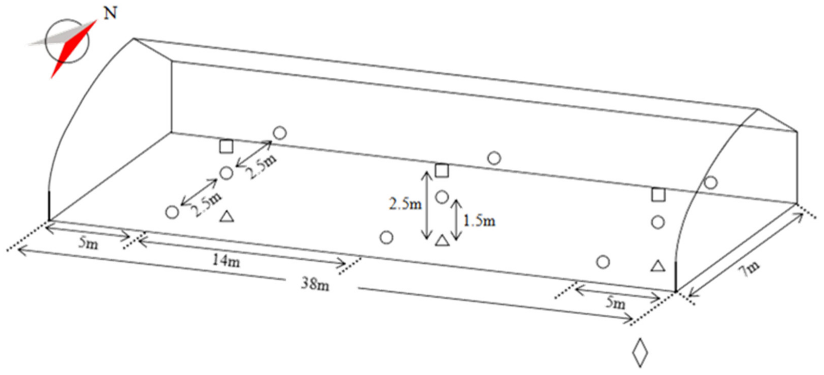
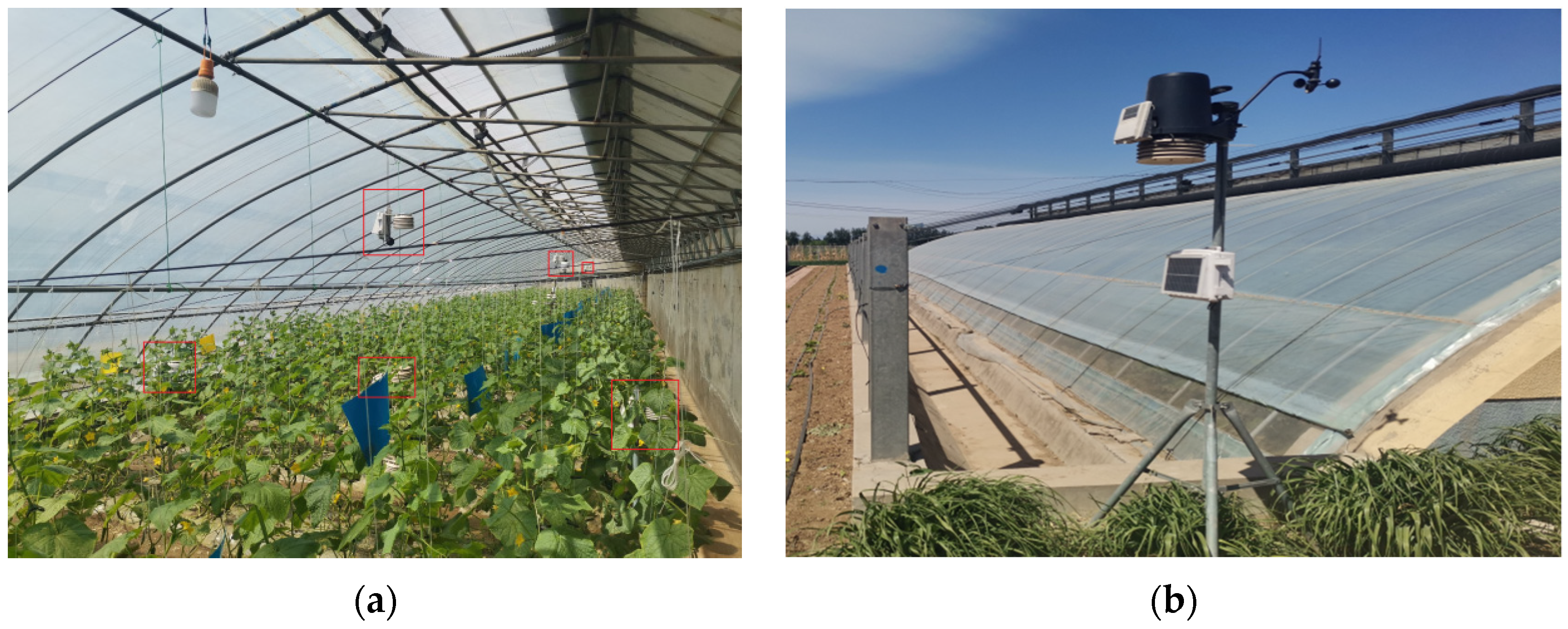
The indoor environmental monitoring nodes (EnviroMonitor Node, Davis Instruments, Hayward, CA, USA) were placed at a height of 1.5 m. The wireless temperature and humidity sensors were at a height of 2.5 m, and the soil temperature and water potential sensors were buried in the soil layer of 0.15–0.2 m below the second node in each column (Figure 1 and Figure 2a). The weather station Davis Vantage Pro2 (Davis Instruments, Hayward, CA, USA) was located in an open space near the southeast boundary of the greenhouse, and it could automatically communicate with monitoring nodes in the greenhouse under the wireless LAN connection to realize the upload and storage of data (Figure 1 and Figure 2b). The data acquisition interval was 15 min, and the data was downloaded from the server once a month. Meanwhile, it could acquire data on various outside environmental factors such as wind speed, rainfall, atmospheric pressure, etc.
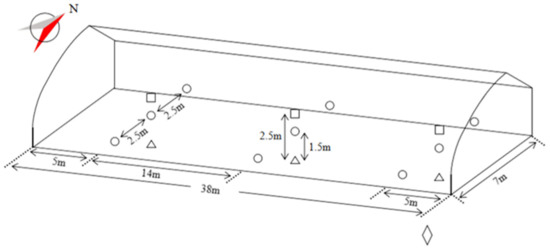
Figure 1.
The schematic diagram of the experiment sensors equipment installation. represents the 1.5 m high environmental monitoring nodes, represents the 2.5 m high wireless temperature and humidity sensors, represents the soil temperature and water potential sensors in the soil layer of 0.15–0.2 m, represents the weather station; N means north.
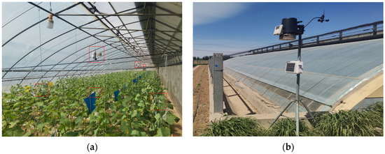
Figure 2.
Photos of equipment installation. (a) Photo of the indoor sensors. (b) Photo of the weather station.
Taking the occurrence of cucumber downy mildew in the solar greenhouse as the research object, we conducted weekly surveys and observations until the early symptoms of cucumber downy mildew (light yellow water-stained polygonal disease spots on the leaves) appear, determined the center of the disease occurrence, and recorded the time of the first onset. After that, the cycle was changed to a 3~4 d survey interval. According to the Pesticide-Guidelines for the Field Efficacy Trials (I)—Fungicides Against Downy Mildew of Cucumber (GB/T 17980.26-2000) [28], the diagonal five-point sampling method was adopted for the fixed-point plant investigation.
2.2. Dataset Construction
2.2.1. Model Variables Selection
According to the law of cucumber downy mildew occurrence and spread, it can be known that the air temperature and relative humidity are the important factors affecting the occurrence of the disease. In addition, the wet leaves will accelerate the infection of pathogens [1,2,10,29,30] when the relative humidity is too high. The solar radiation [2,30] will affect the activity of sporangia, and cause the soil temperature change. The pathogens that are dormant in the soil begin to disperse, causing the primary infection of the disease. Through reading and comparing a large number of references and combining them with the actual situation, we selected the temperature, relative humidity, soil temperature, solar radiation, and the situation of leaf wetness as the input independent variables of the model. The situation of disease occurrence was used as the output dependent variable of the model. Among them, the situation of leaf wetness was converted from the relative humidity at 2.5 m through the threshold, and 89% was selected as the relative humidity threshold [31], that is, if the relative humidity was greater than or equal to 89%, the leaves were defined as wet, and less than 89% was defined as the leaves were not wet. Model variables setting, units or descriptions, and symbols definition are shown in Table 1.

Table 1.
Model variables setting, units or descriptions, and symbols definition.
2.2.2. Data Pre-Processing
We used PyCharm 2019.3 and Python 3.7.11 to perform mean value calculation, variables name definition, and data format processing on the original environmental data. For missing data caused by equipment aging, damage, etc., linear interpolation was used to process the missing values. The equation used was the following:
where X0, Y0, X1, Y1 are known sample data. X is the data between X0 and X1. Y is the missing data corresponding to X to be interpolated. The processing of missing values through linear interpolation was a crucial step in data pre-processing, which not only ensured the completeness of the data, but also reduced the errors that may be caused by missing data.
After threshold conversion of the relative humidity, the disease occurrence data was added, and the characteristic variables were divided and the labels were set as shown in Table 1. As these environmental data had different dimensional units and the same category data difference was small and the distribution was close, the Min-Max normalization method was adopted. The normalization equation is the following:
where Xi is all sample data (i = 1, 2, 3, …, n). Xmin is the minimum value among all sample data. Xmax is the maximum value among all sample data. X* is the normalized results. The data was transformed into supervised data through normalization processing, and the dimension data was transformed into dimensionless data between [0, 1], thereby eliminating the influence between data dimensions and the inter-indices comparability, to reduce the amount of calculation, increase the speed of calculation, and improve the accuracy and performance of the model.
Among them, LW was the 0/1 classification feature of whether the leaves were wet or not, and Disease was the 0/1 classification label of whether the Disease occurred or not. The data had been in the range [0, 1], so normalization was not required. After normalization, the model dataset was obtained. A total of 70% of the total data was divided into the model training set (8279 pieces) for the model to learn the information in the data, and the remaining 30% was the model test set (3548 pieces), used to test the effectiveness of the validation model on data learning and made classification predictions.
2.3. Disease Occurrence Prediction Model Development
Deep learning is the process of continuously adjusting the network and enabling the model to perform various nonlinear transformations on the input variables to effectively fit the output. The influence of different parameters on the gradient descent speed of the model and the results may also be different, so it is necessary to continuously test the network, and choose the best optimizer and learning rate to optimize and improve the model [32,33]. The Keras deep learning framework is an advanced neural network Application Programming Interface (API) written by Python, which included neural network layers, loss functions, optimizers, activation functions, and other modules for model construction, training, debugging, and evaluation. It was used for the rapid construction of the model framework. KNN [34] (K-Nearest Neighbors Classification) is a commonly used classification algorithm in data mining, it represents the data to be classified by its nearest K neighbors values, and realizes the division of classification results. ANN [35] (Artificial Neural Network) is a traditional neural network algorithm, and it is the simplest neural network structure, with only a single hidden layer. This experiment was carried out in a GPU environment. The Keras deep learning framework (TensorFlow as the backend) was used to complete the construction of the model and debug the learning process, and compare it with the KNN classification algorithm and the ANN algorithm. The model training environment and parameters configuration are shown in Table 2 shown.
Table 2.
The model training environment and parameters configuration.
This model consisted of two LSTM layers, a Dropout layer, and a Dense layer. Among them, LSTM defined the three-dimensional shape (None, 1, 5) of the input dataset and conducted preliminary learning on a large amount of input data by increasing the number of neuron nodes (None, 1, 128). None (None, 1, 5) represents the number of every time input data, 1 represents a label category (the situation of disease occurrence), and 5 represents the number of five features (five independent variables we selected). Here, 128 represents the number of defined network units. The dropout layer was a regularization operation on the network, whose contained useless information network units will be randomly hidden or discarded during the training process to prevent the model from overfitting. The LSTM_1 had the same scale as the LSTM layer after regularization. It stored, memorized, and classified information related to the features and labels of the training dataset and saved the remaining network units for data dimensionality reduction (None, 64). The Dense layer was a fully connected layer, which could map the feature classification results (None, 1) of the upper network through nonlinear changes to the output space, and then improve the classification accuracy of the model. The structure diagram of the disease occurrence prediction model is shown in Figure 3.
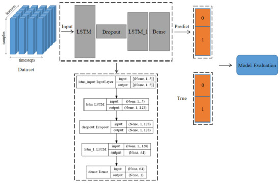
Figure 3.
The structure diagram of disease occurrence prediction model.
According to the learning effect of the training set, the above model used the test set features to predict the situation of disease occurrence (Not Occurrence: 0; Occurrence: 1), compared the predicted label with the actual label, and calculated the evaluation indicators of the corresponding prediction model.
2.4. Model Evaluation Indicators
The prediction model of time-series environmental factors used RMSE (Root Mean Square Error) and MAE (Mean Absolute Error) as evaluation indicators to describe the error between the true value and the predicted value. The disease occurrence prediction model used Accuracy, Precision, Recall, F1-score and ROC (Receiver Operating Characteristic) curve, AUC (Area Under Curve) value, confusion matrix, and k value (Kappa coefficient) as performance evaluation indicators.
The calculated equation used were the following:
where Oi is the true value. Yi is the predicted value. n is the total number of samples.
Accuracy represents the proportion of the samples that are correctly predicted in the total sample. Precision represents the proportion of the samples that are predicted to be correct in the sample. Recall represents the proportion of the samples that predicted the disease in the actual disease sample F1-score is a comprehensive evaluation indicator combined with Precision and Recall. The calculated equation used were the following:
ROC curve is a graph obtained by using FPR (False Positive Rate) as the abscissa and TPR (True Positive Rate) as the ordinate to show the classification effect of the model. The AUC value is the area under the ROC curve. The closer its value is to 1, the higher the classification performance of the model. The calculated equation used were the following:
The confusion matrix is a visual evaluation indicator that displays the model classification results through a matrix of n rows × n columns. The k value is a consistency check method, and the calculation result is usually between 0 and 1, which is calculated through the numerical calculation of each matrix to measure the classification prediction accuracy. The k value consistency classification criteria are shown in Table 3. The calculated equation used are the following:
Table 3.
The k value consistency classification criteria.
In the above Equations (5)–(13), TP means True Positive, which refers to samples that are actually positive and predicted to be positive. FP means False Positive, refers to samples that are actually negative and predicted to be positive. TN means True Negative, refers to samples that are actually negative and predicted to be negative. FN means False Negative, refers to samples that are actually positive and predicted to be negative. P0 means the observation consistency, Pe means the chance consistency.
3. Results
3.1. Time-Series Environmental Factors Prediction Results
According to the time-series environmental factors data acquired by the sensors, the missing data was processed through linear interpolation, and the four model independent variables were predicted including the temperature (Temp), relative humidity (RH), soil temperature (ST), and solar radiation (SR) in the greenhouse. The results are shown in Figure 4.
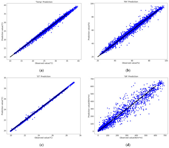
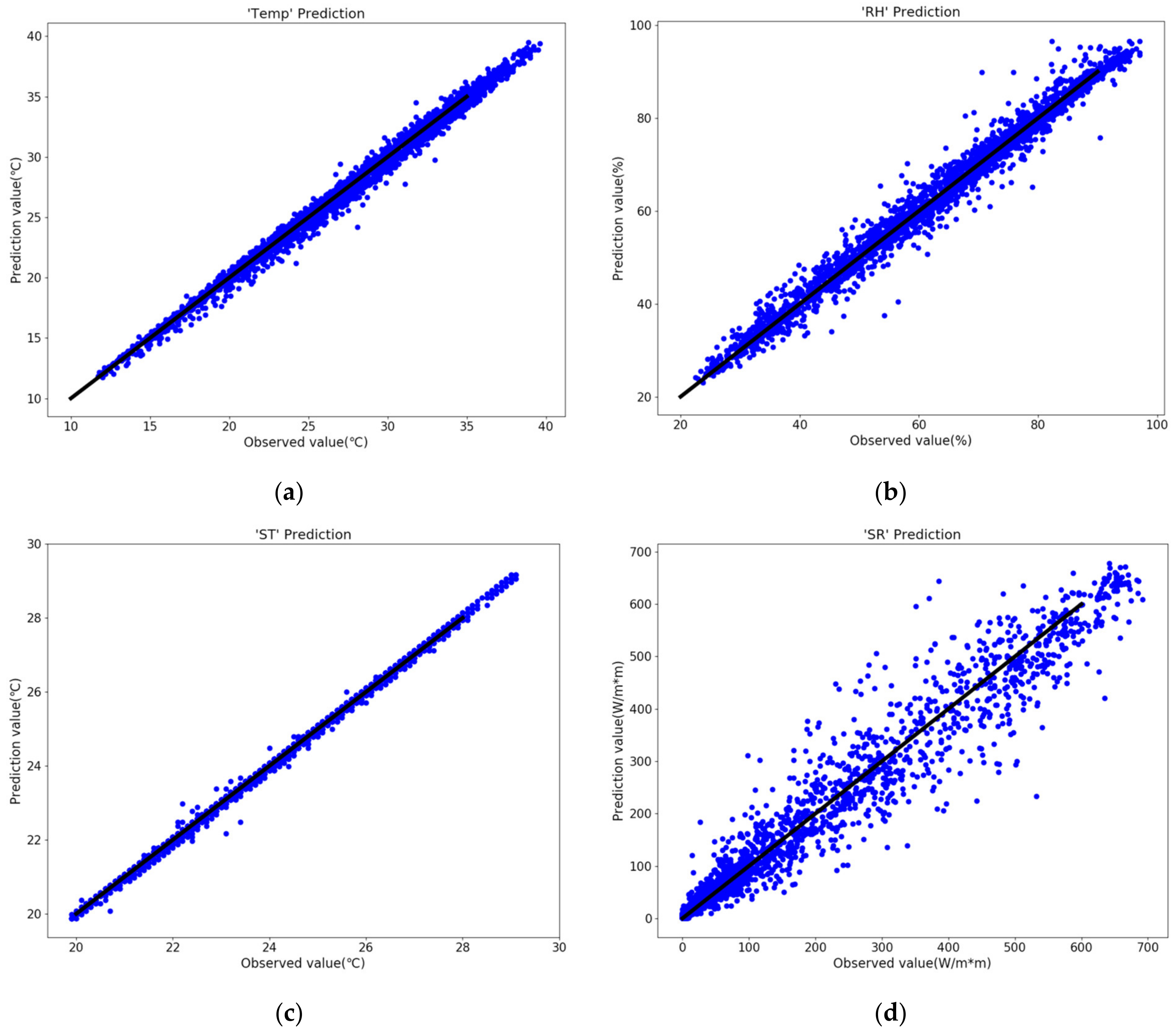
Figure 4.
The solar greenhouse internal environmental factors prediction results. (a) Temp, (b) RH, (c) ST, (d) SR.
The results in Figure 4 and Table 4 shows that the forecasted results of the four environmental factors were consistent with the true value distributions, and R2 (R-Squared) were all above 0.95. Among them, the ST variable predicted the best results, e.g., R2 = 0.9982, RMSE = 0.08 °C, and MAE = 0.05 °C, and within acceptable error range. The results and error level reflected that the model was reliable in predicting time-series environmental factors in the solar greenhouse, and verifying that the model had high accuracy. The disease occurrence prediction model could be further developed through model debugging.
Table 4.
Error evaluation indicators of environmental factors prediction results.
3.2. Model Debugging Results
After threshold conversion of relative humidity, disease occurrence data was added and normalized the data. In order to make the model have the best performance, we selected four good performance and commonly used optimizers for debugging the parameters, when the learning rate was the default value of 0.001, selected the optimizer with the best results. Then for this best performing optimizer, we set different learning rates for it to compare which is optimal, as shown in Table 5.
Table 5.
Different optimizers and learning rates debugging results.
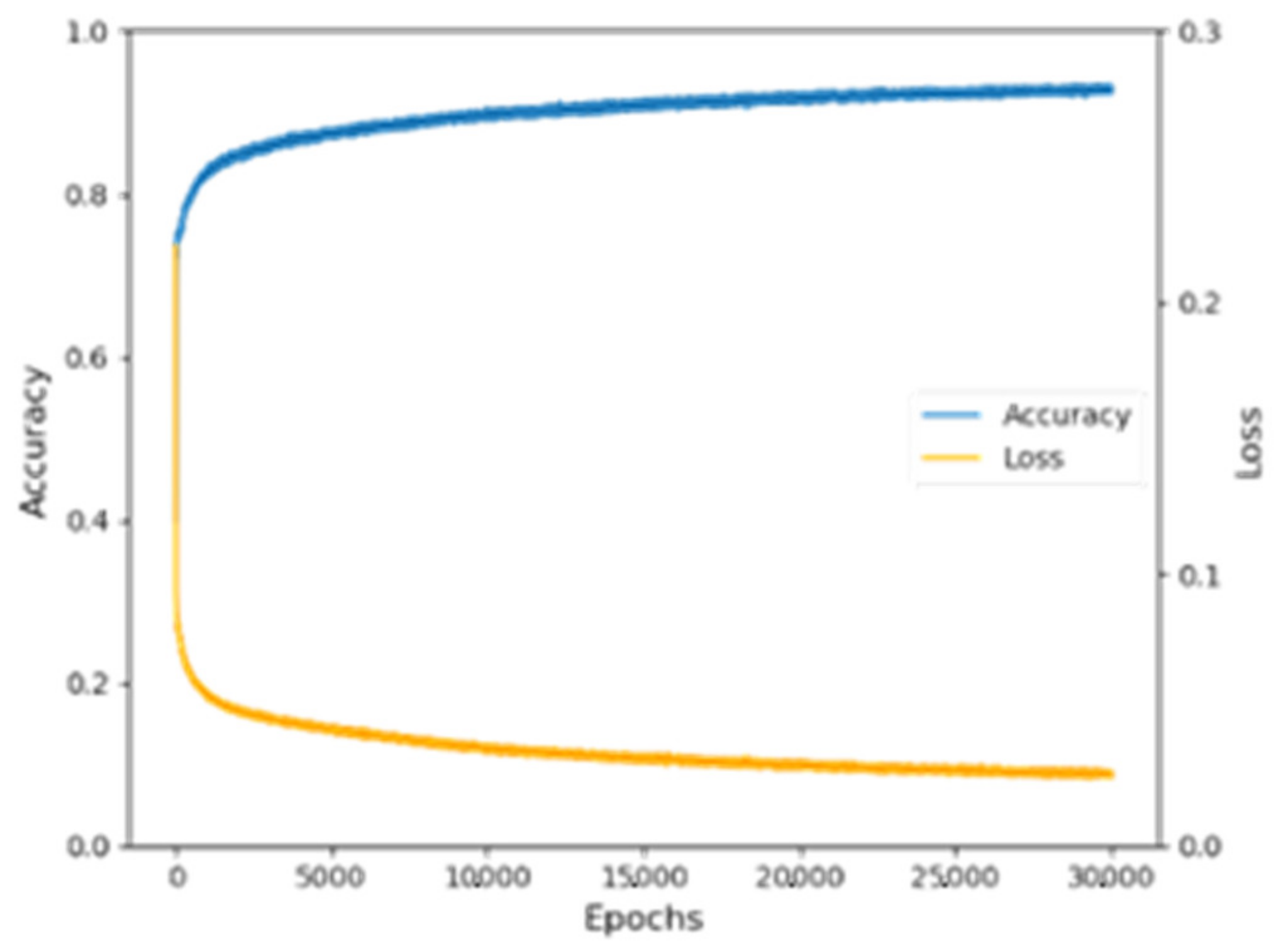
It could be seen that the training set and test set accuracy of the Adam optimizer with a learning rate of 0.001 were the highest among the four optimizers, with a training set accuracy of 95.99% and a test set accuracy of 89.91%. According to the debugging results, this model chose Adam (LR = 0.001) as the optimizer. During the training process, the training set accuracy and loss value rise and fall with epochs are shown in Figure 5.
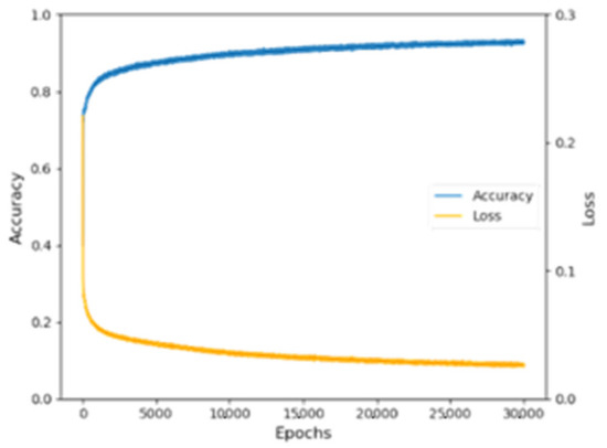
Figure 5.
Variation diagram of the training set accuracy and Loss value.
Since the two represent the quality of the data learning and the error in the model convergence process, the results showed that the training set accuracy and Loss value change were stable and had good results. The Loss value was 0.0159, which indicated that the model had high robustness.
3.3. Disease Occurrence Prediction Results for Different Models
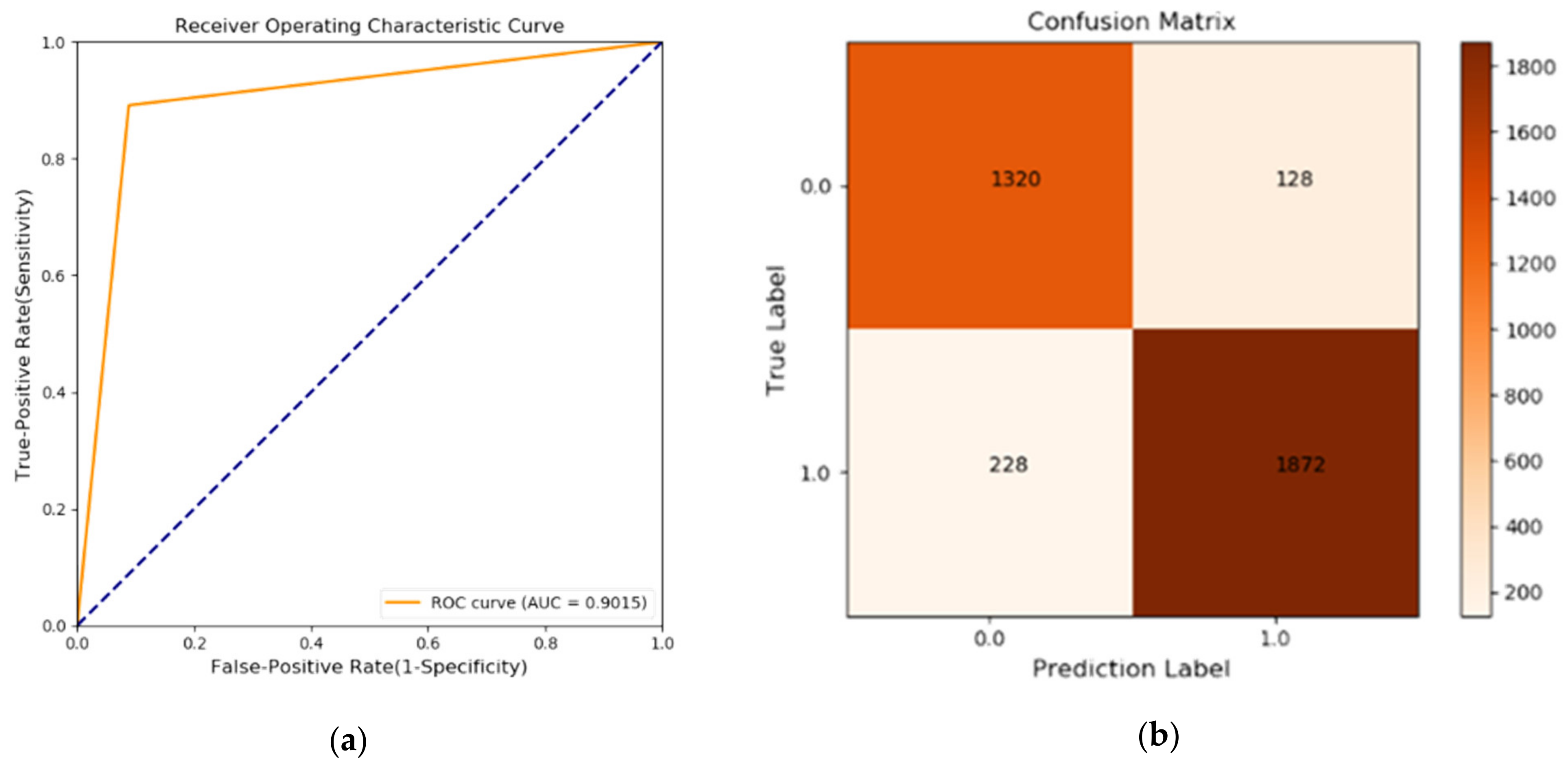
By drawing the ROC curve and confusion matrix, calculating the AUC value and Kappa coefficient, the classification situation and prediction results were evaluated, as shown in Figure 6.

Figure 6.
Disease occurrence prediction model classification indicators. (a) ROC curve. (b) confusion matrix.
From the figure, AUC = 0.9015, indicated that the model classification effect was better; according to the confusion matrix, the ordinate and abscissa were actual disease not occurrence (0) and disease occurrence (1) and predicted disease not occurrence (0) and disease occurrence (1), respectively. The total number in the four matrices was the number of test set 3548 pieces (where TN = 1320, TP = 1872, FN = 228, FP = 128). According to Equations (11)–(13), the k value was 0.80. The result obtained from the k value consistency classification criteria in Table 3 was that the prediction accuracy had substantial consistency, which showed that the accuracy of the prediction of the model was at a high level.
As shown in Table 6, by comparing the evaluation indicators of the LSTM model selected in this article with the KNN classification algorithm and the ANN algorithm model evaluation indicators established based on Keras, the LSTM model predicted the disease occurrence Accuracy, Precision, Recall, and F1-score of 90, 94, 89, and 91%, respectively. It could be seen that these indicators were significantly higher than the indicators of the KNN model and the ANN model, indicating that the LSTM method had obvious advantages over the KNN and ANN methods. The model predicted the occurrence of disease in the verification data better and had a high classification accuracy, indicating that the model had high performance.
Table 6.
Comparison of LSTM, KNN, and ANN model evaluation indicators.
4. Discussion
This article developed a cucumber downy mildew prediction model based on the data of environmental factors in the solar greenhouse. However, this was obtained under two assumptions. The first assumption was that there had been pathogens in the greenhouse. Infection of pathogens is the root cause of cucumber downy mildew. They may be via wind-borne sporangia from outside into the greenhouse [1,2] or maybe always left in the greenhouse on plant residues or soil. As the model was the two-class prediction of whether the disease occurred, this article did not trace the pathogens’ source and did not study the different pathogenic mechanisms presented by different sporangia concentrations. Obviously, in the process of disease investigation, the occurrence of cucumber downy mildew confirmed this assumption. In addition, the cucumber variety we selected was susceptible to disease in previous years, and thus meets the condition that the hosts can be infected. That is, the existence of pathogens, the climate environment suitable [9,10,29] for the dispersal of pathogens [1,2,30] in the greenhouse, and the sensitive host plant tissues together led to the disease epidemic. The second assumption was to ignore the impact on cucumber growth caused by manual management. Because if human factors cause drastic changes in the greenhouse climate environment, data acquisition, and environmental factors prediction results will be unavailable and will affect disease progression [36] and disease prediction accuracy. Of course, we will ensure that the opening and closing time of greenhouse vents and field management operations are consistent and orderly every day, except for sudden changes in external weather that require separate management measures.
This article started from the time of onset of the disease symptoms, divided the growing season into pre-onset and post-onset, constructed an LSTM neural network structure based on the Keras deep learning framework, and developed a prediction model for the temperature, relative humidity, soil temperature, and solar radiation in the solar greenhouse. Based on the evaluation results of the environmental factors prediction model (Figure 4), we can see that LSTM has achieved good results in the processing of time-series data, this is similar to Liu’s [11] research. Therefore, through parameter adjustment, model debugging, and adding the situation of leaf wetness and the situation of disease occurrence data, it can be used to develop the disease occurrence prediction model. Compared with the existing prediction models [7,8,9,10,13] for cucumber downy mildew, this model is more advantageous in analyzing time-series data closely related to the occurrence of the disease, with higher accuracy and wider applicability.
The LSTM was the first time to be applied in the prediction of cucumber downy mildew in solar greenhouses, and it has some shortcomings in this study. Since each piece of data in this experiment represents the data acquired by sensors every 15 min, the error in the prediction (Figure 6) may be because since the features between the data within 15 min were too detailed or small, and the model was not easy learning and distinguishing results in the inability, resulting in classification errors. However, it was precisely because of the small data acquisition interval that the total number of classification errors was also accumulated in units of 15 min, which greatly improved the precise range of disease occurrence time and facilitates farmers to take management and prevention measures in advance [1,3,29,31,36]. At the same time, model classification performance can be improved through model regularization, parameter optimization, and learning rate adjustment [32,33]. This is also the reason for the adjustment of the parameters and the concrete manifestation of the result obtained after the adjustment.
In future work, the pathogenic sporangia growth curve, incidence rate, disease index, and other data can be used as the basis and distinguishing standard of disease occurrence level [2] to explore their changes and connections. At the same time, combined with the prediction model of environmental factors in the greenhouse [11], realize the short-term environmental factors in the future using the data acquired from these predictions. Then, develop a disease prediction system, through the data of future short-term environmental factors, the disease occurrence prediction model is used to predict the future occurrence of disease, and the two-classification problem of predicting the occurrence of the disease is extended to a multi-classification problem of predicting the severity of disease occurrence, to better help farmers to take prevention or control measures in advance. We can also place the disease occurrence prediction model on the platform [37], which can automatically call and analyze data to realize the visual path of the dynamic spread [38] of the disease for users’ reference. At the same time, we will increase the verification experiments in different greenhouses, different seasons and different varieties to expand the scope of application of the model and improve the research on the prediction of cucumber diseases in solar greenhouses.
Author Contributions
Conceptualization, H.L. and M.L.; Methodology, K.L., H.L. and M.L.; Software, K.L.; Validation, K.L.; Formal analysis, K.L.; Investigation, K.L. and C.Z.; Resources, H.L. and M.L.; Data curation, K.L. and C.Z.; Writing—original draft preparation, K.L.; Writing—review and editing, K.L.; Visualization, K.L.; Manuscript revising, H.L. and M.L.; Study design, X.Y., M.D. and M.L.; Supervision, X.Y., M.D., H.L. and M.L.; Project administration, X.Y., M.D., H.L. and M.L.; Funding acquisition, M.L. All authors have read and agreed to the published version of the manuscript.
Funding
This work was funded by the Science and Technology Innovation Capacity Building Project of Beijing Academy of Agriculture and Forestry Sciences (No. KJCX20211002); Youth Program of National Natural Science Foundation of China (31401683); National Key R&D Program of China (SQ2020YFF0418305), and the FP7 Framework Program (PIRSES-GA-2013-612659).
Institutional Review Board Statement
Not applicable.
Informed Consent Statement
Not applicable.
Data Availability Statement
Not applicable.
Conflicts of Interest
The authors declare no conflict of interest.
References
- Lebeda, A.; Cohen, Y. Cucurbit downy mildew (Pseudoperonospora cubensis)-biology, ecology, epidemiology, host-pathogen interaction and control. Eur. J. Plant Pathol. 2011, 129, 157–192. [Google Scholar] [CrossRef]
- Granke, L.L.; Morrice, J.J.; Hausbeck, M.K. Relationships between airborne Pseudoperonospora cubensis sporangia, environmental conditions, and cucumber downy mildew severity. Plant Dis. 2014, 98, 674–681. [Google Scholar] [CrossRef] [Green Version]
- Rotem, J.; Cohen, Y.; Bashi, E. Host and environmental influences on sporulation in vivo. Annu. Rev. Phytopathol. 1978, 16, 83–101. [Google Scholar] [CrossRef]
- Sankaran, S.; Mishra, A.; Ehsani, R.; Davis, C. A review of advanced techniques for detecting plant diseases. Comput. Electron. Agric. 2010, 72, 1–13. [Google Scholar] [CrossRef]
- Li, S.; Guo, Z.C.; Wang, C.; Chen, T.N.; Yuan, Z.G. A review of the application of information technology in monitoring and early warning of crop diseases and insect pests. Jiangsu Agric. Sci. 2018, 46, 1–6, (In Chinese with English abstract). [Google Scholar]
- Wang, X.Y. Methods Study on Early Warning of Facility Vegetable Disease Based on Disease Triangle Theory. Ph.D. Thesis, China Agricultural University, Beijing, China, 2018. (In Chinese with English abstract). [Google Scholar]
- Pouzeshimiyab, B.; Fani, S.R. Epidemiology and Aerobiology of Pseudoperonospora cubensis in northwest Iran. Ital. J. Agrometeorol. 2020, 25, 109–116. [Google Scholar]
- Neufeld, K.N.; Keinath, A.P.; Ojiambo, P.S. Evaluation of a Model for Predicting the Infection Risk of Squash and Cantaloupe by Pseudoperonospora cubensis. Plant Dis. 2018, 102, 855–862. [Google Scholar] [CrossRef] [Green Version]
- Zhao, C.J.; Li, M.; Yang, X.T.; Sun, C.H.; Qian, J.P.; Ji, Z.T. A data-driven model simulating primary infection probabilities of cucumber downy mildew for use in early warning systems in solar greenhouses. Comput. Electron. Agric. 2011, 76, 306–315. [Google Scholar] [CrossRef]
- Li, M.; Zhao, C.J.; Yang, X.T. Towards an Early Warning Framework of Greenhouse Vegetable Diseases—A Case of Cucumber Downy Mildew. Chin. Agric. Sci. Bull. 2010, 26, 324–331, (In Chinese with English abstract). [Google Scholar]
- Liu, Y.W.; Li, D.J.; Wan, S.H.; Wang, F.; Dou, W.C.; Xu, X.L.; Li, S.C.; Ma, R.; Qi, L.Y. A long short-term memory-based model for greenhouse climate prediction. Int. J. Intell. Syst. 2022, 37, 135–151. [Google Scholar] [CrossRef]
- Liakos, K.G.; Busato, P.; Moshou, D.; Pearson, S.; Bochtis, D. Machine learning in agriculture: A review. Sensors 2018, 18, 2674. [Google Scholar] [CrossRef] [Green Version]
- Jia, Y. A Data-driven Monitoring and Early Warning System of Cucumber Downy Mildew in Greenhouse. Master’s Thesis, Shandong Agricultural University, Taian, China, 2019. (In Chinese with English abstract). [Google Scholar]
- Bhatia, A.; Chug, A.; Prakash Singh, A. Application of extreme learning machine in plant disease prediction for highly imbalanced dataset. J. Stat. Manag. Syst. 2020, 23, 1059–1068. [Google Scholar] [CrossRef]
- Xu, W.; Wang, Q.; Chen, R. Spatio-temporal prediction of crop disease severity for agricultural emergency management based on recurrent neural networks. GeoInformatica 2018, 22, 363–381. [Google Scholar] [CrossRef]
- Hsieh, J.Y.; Huang, W.; Yang, H.T.; Lin, C.C.; Fan, Y.C.; Chen, H. Building the Rice Blast Disease Prediction Model Based on Machine Learning and Neural Networks; EasyChair: Manchester, UK, 2019. [Google Scholar]
- Hochreiter, S.; Schmidhuber, J. Long short-term memory. Neural Comput. 1997, 9, 1735–1780. [Google Scholar] [CrossRef] [PubMed]
- Xu, L.; Diao, Z.; Wei, Y. Non-linear target trajectory prediction for robust visual tracking. Appl. Intel. 2021, 1–15. [Google Scholar] [CrossRef]
- Muthukumar, P.; Cocom, E.; Holm, J.; Comer, D.; Lyons, A.; Burga, I.; Hasenkopf, C.; Pourhomayoun, M. Real-Time Spatiotemporal Air Pollution Prediction with Deep Convolutional LSTM Through Satellite Image Analysis. In Advances in Data Science and Information Engineering; Stahlbock, R., Weiss, G.M., Abou-Nasr, M., Yang, C.Y., Arabnia, H.R., Deligiannidis, L., Eds.; Springer: Cham, Switzerland, 2021; pp. 315–326. [Google Scholar]
- Memarzadeh, G.; Keynia, F. Short-term electricity load and price forecasting by a new optimal LSTM-NN based prediction algorithm. Electr. Power Syst. Res. 2021, 192, 106995. [Google Scholar] [CrossRef]
- Xia, D.; Zhang, M.; Yan, X.; Bai, Y.; Zheng, Y.; Li, Y.; Li, H. A distributed WND-LSTM model on MapReduce for short-term traffic flow prediction. Neural Comput. Appl. 2021, 33, 2393–2410. [Google Scholar] [CrossRef]
- Moghar, A.; Hamiche, M. Stock market prediction using LSTM recurrent neural network. Procedia Comput. Sci. 2020, 170, 1168–1173. [Google Scholar] [CrossRef]
- Poornima, S.; Pushpalatha, M. Drought prediction based on SPI and SPEI with varying timescales using LSTM recurrent neural network. Soft Comput. 2019, 23, 8399–8412. [Google Scholar] [CrossRef]
- Shin, S.; Lee, M.; Song, S.K. A Prediction Model for Agricultural Products Price with LSTM Network. J. Korea Contents Assoc. 2018, 18, 416–429. [Google Scholar]
- Cao, J.; Zhang, Z.; Tao, F.; Zhang, L.; Luo, Y.; Zhang, J.; Han, J.; Xie, J. Integrating multi-source data for rice yield prediction across china using machine learning and deep learning approaches. Agric. Forest Meteorol. 2021, 297, 108275. [Google Scholar] [CrossRef]
- Kim, Y.; Roh, J.H.; Kim, H.Y. Early forecasting of rice blast disease using long short-term memory recurrent neural networks. Sustainability 2018, 10, 34. [Google Scholar] [CrossRef] [Green Version]
- Xiao, Q.; Li, W.; Kai, Y.; Chen, P.; Zhang, J.; Wang, B. Occurrence prediction of pests and diseases in cotton on the basis of weather factors by long short term memory network. BMC Bioinf. 2019, 20, 688. [Google Scholar] [CrossRef]
- Ministry of Agriculture of the People’s Republic of China. Pesticide-Guidelines for the Field Efficacy Trials(I)—Fungicides Against Downy Mildew of Cucumber; (GB/T 17980.26-2000); Ministry of Agriculture of the People’s Republic of China: Beijing, China, 2000.
- Cohen, Y. The combined effects of temperature, leaf wetness, and inoculum concentration on infection of cucumbers with Pseudoperonospora cubensis. Can. J. Bot. 1977, 55, 1478–1487. [Google Scholar] [CrossRef]
- Savory, E.A.; Granke, L.L.; Quesada-Ocampo, L.M.; Varbanova, M.; Hausbeck, M.K.; Day, B. The cucurbit downy mildew pathogen Pseudoperonospora cubensiss. Mol. Plant Pathol. 2011, 12, 217–226. [Google Scholar] [CrossRef] [PubMed]
- Li, M.; Zhao, C.J.; Qiao, S.; Qian, J.P.; Yang, X.T. Estimation model of leaf wetness duration based on canopy relative humidity for cucumbers in solar greenhouse. Trans. Chin. Soc. Agric. Eng. 2010, 26, 286–291, (In Chinese with English abstract). [Google Scholar]
- Faris, H.; Aljarah, I.; Mirjalili, S. Training feedforward neural networks using multi-verse optimizer for binary classification problems. Appl. Intell. 2016, 45, 322–332. [Google Scholar] [CrossRef]
- Hu, W.J.; Fan, J.; Du, Y.X.; Li, B.S.; Xiong, N.; Bekkering, E. MDFC-ResNet: An Agricultural IoT System to Accurately Recognize Crop Diseases. IEEE Access 2020, 8, 115287–115298. [Google Scholar] [CrossRef]
- Guo, G.; Wang, H.; Bell, D.; Bi, Y.; Greer, K. KNN model-based approach in classification. In OTM Confederated International Conferences, On the Move to Meaningful Internet Systems; Springer: Berlin/Heidelberg, Germany, 2003; pp. 986–996. [Google Scholar]
- Wang, S.C. Artificial neural network. In Interdisciplinary Computing in Java Programming; Springer: Boston, MA, USA, 2003; pp. 81–100. [Google Scholar]
- Palti, J.; Cohen, Y. Downy mildew of cucurbits (Pseudoperonospora cubensis): The fungus and its hosts, distribution, epidemiology and control. Phytoparasitica 1980, 8, 109–147. [Google Scholar] [CrossRef]
- Kim, S.; Lee, M.; Shin, C. IoT-based strawberry disease prediction system for smart farming. Sensors 2018, 18, 4051. [Google Scholar] [CrossRef] [Green Version]
- Ojwang, A.M.E. Network Models for the Dispersal of Pseudoperonospora cubensis and Spread of Cucurbit Downy Mildew in the Eastern United States. Ph.D. Thesis, North Carolina State University, Raleigh, NC, USA, 2021. [Google Scholar]

Publisher’s Note: MDPI stays neutral with regard to jurisdictional claims in published maps and institutional affiliations. |
© 2022 by the authors. Licensee MDPI, Basel, Switzerland. This article is an open access article distributed under the terms and conditions of the Creative Commons Attribution (CC BY) license (https://creativecommons.org/licenses/by/4.0/).