Article

Comparative Analysis of Pasture Soil Fertility in Semiarid Agro-Silvo-Pastoral Systems

by
Francisco J. Moral
1,*,
João M. Serrano
2,
Francisco J. Rebollo
3,
Ricardo F. M. Teixeira
4 and
Tiago Domingos
4
1
Departamento de Expresión Gráfica, Escuela de Ingenierías Industriales, Universidad de Extremadura, Avda. de Elvas, s/n., 06006 Badajoz, Spain
2
MED—Mediterranean Institute for Agriculture, Environment and Development & CHANGE—Global Change and Sustainability Institute, Departamento de Engenharia Rural, Escola de Ciências e Tecnologia, Universidade de Évora, Pólo da Mitra, Ap. 94, 7006-554 Évora, Portugal
3
Departamento de Expresión Gráfica, Escuela de Ingenierías Agrarias, Universidad de Extremadura, Avda. Adolfo Suárez, s/n., 06007 Badajoz, Spain
4
MARETEC—Marine, Environment and Technology Centre, LARSyS, Instituto Superior Técnico, Universidade de Lisboa, Av. Rovisco Pais, 1, 1049-001 Lisboa, Portugal
*
Author to whom correspondence should be addressed.
Agronomy 2022, 12(11), 2711; https://doi.org/10.3390/agronomy12112711
Submission received: 25 August 2022 / Revised: 24 October 2022 / Accepted: 26 October 2022 / Published: 1 November 2022
(This article belongs to the Section Grassland and Pasture Science)

Abstract

:
Dryland pastures are usually on soils with a low fertility. However, a high spatial variability is apparent in pasture soils. In consequence, the application of inputs should be based on the particular characteristics of each field and their within-field variability. In this study, a comparative analysis of seven experimental fields (agro–silvo–pastoral ecosystems) in the southwest of the Iberian Peninsula was performed using a probabilistic and objective model. Some soil properties (the texture, cation exchange capacity, soil apparent electrical conductivity, organic matter, nitrogen, potassium and slope) measured at six sampling locations in each field were consolidated in the model. It was verified that the data fit the model and, later, a ranking of all the sampling locations and, consequently, a ranking of all the experimental fields according to the pasture soil fertility was established. Moreover, another output of the model was a ranking of the soil properties according to their influence on the soil fertility: the topographical property, the slope, was the most influential as it is related to the level of other important soil properties, as the textural components. Two fields, Cubillos and Grous, had the highest overall soil fertility levels because the soil samples in these fields were very fertile. However, some samples in the other five fields were also in the group of the most fertile, denoting the existence of an important spatial variability within each field. The proposed method is a rational way to improve the efficiency of the use of fertilisers by adjusting them to the soil pasture fertility.

1. Introduction

The southwest of the Iberian Peninsula has a semiarid climate. The water deficit is the main limitation in the rainfed crops. Irrigation is necessary in many cases to obtain a minimum crop yield and, in consequence, an economic profitability. However, a unique Mediterranean evergreen oak woodland, called montado in Portugal or dehesa in Spain, extends on an important area, approximately 2.5 million ha [1]. It is an anthropogenic ecosystem of a high conservation and socio-economic value, with a high biodiversity. Quercus suber and Quercus ilex species are their main systems of mixed trees with scattered shrubs and natural biodiverse pastures (such as grasses and legumes). Many goods are produced in these systems, such as cork, firewood, honey, etc. However, the essential utilisation of this ecosystem is for grazing. The production system is extensive and animals are essentially fed by pastures and shrubs. The pasture yield and quality is determined by the soil fertility [2,3]. However, these soils have a low fertility because of intense erosion, so shallow, acidic, and stony soils have a low nutrient content [4]. Still, many soil properties exhibit an important spatial variability [2,3,5], since different chemical, physical, and biological processes interact with different intensities and simultaneously [6,7]. These variable spatial patterns in many soil properties lead to a significant variability in the fertility that causes heterogeneity in the forage yield and quality.
Pasture degradation derived from inadequate soil and pasture management practices reduces the economic return of this agro–silvo–pastoral ecosystem because animal feed supplementation is increased. Moreover, in the current context of climate change, which is particularly intense in this region [8], the importance of an adequate management is essential for its conservation. The delineation of zones with homogeneous permanent soil properties is the most effective management strategy to optimise the pasture productivity and extensive animal production of this agro–silvo–pastoral ecosystem. These sub-regions are known as management zones (MZ) [5,9,10]. The soil fertility and production potential are similar in the MZ because they have a homogeneous combination of soil-landscape attributes and yield-limiting factors [2,10,11]. The main factor that determines the forage yield and quality is the soil fertility, so the knowledge of its variability is essential to propose site-specific management strategies [2].
The accurate delineation of soil fertility patterns is difficult because many factors affecting the pasture yield and quality interact in a complex way. However, any method to characterise them has to take into account the main chemical and physical soil properties, because they affect the pasture biomass the most [12,13]. Consequently, the yield variability is related to the variability on the soil properties, because they determine the plant’s available water and, in turn, the pasture production potential [11].
Although a homogeneous management of the pasture field is a habitual practice when there is no information about the soils and their main properties, the application of the production factors cannot be the same in all the pasture fields. Pasture soil fertility is usually very different not only between the fields but also within each field, so the economic feasibility of these silvo–pastoral ecosystems requires the implementation of strategies which are adapted to each particular field [14].
With the aim of defining the within-field management zones, many studies in agricultural fields were performed to evaluate the different methods [15,16,17], but little research in the pasture field has been reported [18]. However, the same techniques can be used in agricultural and pasture systems to rationally delineate the homogeneous zones in the fields. The most important variables can be integrated with different algorithms as the cluster procedure using fuzzy c-means methods [19], the consideration of the coefficient of variation of the data layers [20] and principal component analysis, which can be combined with the cluster technique [21,22]. Only recently has the use of the Rasch model, an objective and probabilistic model, been proposed as a novel method to consolidate the soil variables. The successful utilisation of the Rasch model to integrate the soil properties has been reported on agricultural fields [23,24] and on pasture soils [3,5,11]. One of the main advantages of the outputs from this model is that results can be easily understood. Moreover, the formulation of this model does not need initial constraints or weights about the variables [25].
This research had these main objectives: to (1) apply the Rasch model, as a measurement tool, to compute the pasture soil fertility in different fields and (2) compare the pasture soil fertility between the fields and within each field.

2. Materials and Methods

2.1. Experimental Fields

This study was performed in seven experimental fields (Table 1), five located in the Alentejo region (southern of Portugal), one in the Beira Interior region of Portugal and one in the Extremadura region (southwestern Spain) (Figure 1). These fields have been cultivated with permanent dryland pastures and there is a low or moderate density plantation of Cork oak or Holm oak. Usually, on a rotational basis, the pastures are used for grazing by pigs, sheep or cattle (Table 1).
The predominant soil type is Cambisol, which is derived from granite [26]. These soils have their parent material with a slight or moderate weathering. Moreover, there are low levels of organic matter, iron compounds, aluminium and illuviated clay. Their texture is mainly sandy (Table 1), with a sand content up to 80%. These pasture soils, not very fertile, are usually utilised for mixed agro–silvo–pastoral systems [13].
The climate is Mediterranean, type Csa [27] according to the Köppen–Geiger classification. The maximum and minimum temperature ranges between more than 40 °C in the summer and 0 °C in the winter. The inter-annual variability of precipitation is very high and it principally falls between October and March, being almost non-existent in the summer. There is a precipitation gradient from the north to the south: in the northern districts, “Portalegre” and “Castelo Branco”, the mean annual rainfall is 950 and 1330 mm, respectively; in the central district, “Évora”, the mean annual precipitation is 567 mm and in the southern district, “Beja”, this value is 430 mm.

2.2. Soil Sample Collection and Analysis

In each pasture field (Figure 1), six sampling locations were taken in a depth range of 0–0.30 m. The samples were collected with a gouge auger and a hammer. Five combined sub-samples collected in an area of 100 m2 (10 m × 10 m) were considered in each sampling location. A global navigation satellite system (GNSS) (Trimble 4700 GPS-RTK, Trimble Navigation Limited, Sunnyvale, CA, USA) was used to georeference all the sample locations. After taking the samples, they were kept in plastic bags. Later, in the laboratory at the University of Évora, all samples were air-dried and were then analysed for their texture with a sedimentographer (Sedigraph 5100, Micrometritics, Norcross, GA 30093-2901, USA). Later, the fine soil fraction was analysed using the standard methods [28]: the total nitrogen content, the TN, was measured by the Kjeldahl method; the Egner–Riehm method was used to extract the K2O, being determined by a flame photometer; the organic matter (OM) was determined, with an infrared detection cell, by combustion and a CO2 measurement; and the neutral ammonium acetate method was used to measure the cation exchange capacity (CEC).
An EM38 non-contact sensor (Geonics Ltd., Mississauga, ON, Canada) was used in the horizontal dipole orientation to conduct the soil apparent electrical conductivity (EC) surveys at each pasture field in October 2019. The two receiver coils were separated by 0.5 m from the transmitter. It provides data from depth ranges of 0.75 m and 0.375 m, but, in this study, only the topsoil data, 0–0.375 m, were used. The device was pulled by an all-terrain vehicle, mounted on a sledge by an all-terrain vehicle, which was equipped with a GNSS device (Trimble RTK/PP-4700 GPS, Trimble Navigation Limited, Sunnyvale, CA, USA), providing simultaneously a topographic survey. The average speed of the vehicle was 2.5 m s−1, performing successive passages across the fields and registering the EC measurements every second. From these EC data, kriged EC maps (shown in Serrano et al. [14]) were generated in each pasture field and the values of EC, at each location where a sample was taken, were obtained from the EC maps. Moreover, using the triangulated irregular network (TIN) interpolation, digital elevation model (DEM) surfaces were produced for each field. These surfaces are also shown in Serrano et al. [14]. The values of the elevation and slope at each sampling location were obtained from the DEMs.

2.3. The Rasch Model

In the item response theory models for the measurement, the probabilistic Rasch model is one of the most powerful [29]. It is a novel measuring tool to define the pasture soil fertility, taking into account the relationship with the potential yield of the pasture biomass. This is a latent variable model with only one measurement parameter [30]. In this case study, the soil locations (subjects) and soil properties (items) are classified according to a single dimension. Moreover, the different data with different units are consolidated into a global variable, called latent variable, making the interpretation of the pasture soil fertility easier.
Before formulating the Rasch model, it is necessary to categorise all the data for achieving an adimensional characterisation. Thus, the initial data were transformed to a common scale and the soil properties were freed from the metric constraints. Five categories were defined for all the soil variables, as it was conducted in many previous studies [3,5,10]. The lowest contribution to the fertility of each measure of a soil property was assigned to class 1 and, on the contrary, the highest contribution to the fertility was assigned to class 5. The assignment of the categories for the soil texture was different as the ideal percentage of each class was a third of the total; in consequence, an interval around 33% of each textural class (sand, silt and clay) corresponds to the maximum categorical value, 5. For the other soil properties, the classes with highest measures have the highest categorical values. The amplitude of the other classes is related to the minimum and maximum values of each property. Finally, the data were arranged in a matrix: each cell, Xni, reflected the category for the soil property i, varying from 1 to 9, at the sampling location n, varying from 1 to 42.
According to the treatise on latent variables, Rasch [31] established that:
P [ Xni = 1 ;   Bn , di ] = e ( B n d i ) 1 + e ( B n d i )
that is, the probability that location n has the influence of the soil property corresponding to item i, is given by the parameters Bn and di. According to (1), the greater the difference (Bn−di), the greater the probability is to be 1. Expression (1) was proposed for the Rasch dichotomous model, which was extended to the polytomous models, that is, cases of more than two categories [32].
In this work, some soil properties which were measured at different sites should be integrated into an overall variable in some pasture fields. The pasture soil fertility, the latent variable, was represented by a straight line, in which the sample locations and soil properties are located along. A logit scale for both Bn and di is used by the Rasch model. By taking the logarithms of (1), it is obtained that:
log (P/(1 − P)) = Bn − di
where P = P[Xni = 1; Bn, di]; and log (P/(1 − P)) is the logit of P. Larger positive values are computed for the locations where the pasture soil fertility is higher or the soil properties with a lower influence on the soil fertility. On the contrary, larger negative values are computed for those soil properties with a higher influence on the pasture soil fertility or locations where the soil fertility is lower. A probability between 0.05 and 0.95 is expected for almost all sampling locations, for each soil property, to be influential on them. Consequently, the values of Bn−di are between −3 and 3 logits when considering (1).
Infit and outfit statistics are used to verify if items fit the model, which involves comparing the observed data with those estimated by the Rasch model. Infit means the inlier-sensitive or information-weighted fit. It is more sensitive to the pattern of responses to items targeted on the latent variable. Outfit means the outlier-sensitive fit. It is more sensitive to responses to items that are far from the expected on the latent variable.
With the aim of estimating how each soil property contributes to the pasture soil fertility measurement, two Chi-square fit statistics, the infit and outfit mean-square (infit and outfit MNSQ) can be computed to compare the observed variance to the expected one. These fit statistics show the size of the randomness, that is, the amount of distortion of the measurement system Their expectation is 1, making acceptable values between 0.6 and 1.5 [33]. Values less than 1.0 indicate that the observations are too predictable, that is, the redundancy, meaning the data overfit the model. Values greater than 1.0 indicate unpredictability and unmodeled noise, meaning the data underfit the model. Moreover, according to Edwards and Alcock [34], the expectations of the mean standardised (ZSTD) infit and outfit values (the sum of the squares standardised residuals given as Z-statistics) are 0, making acceptable values between −3 and 2. They show the significance of the data, if the data actually did fit the model. Values less than 0 indicate that the observations are too predictable and more than 0 indicates a lack of predictability.
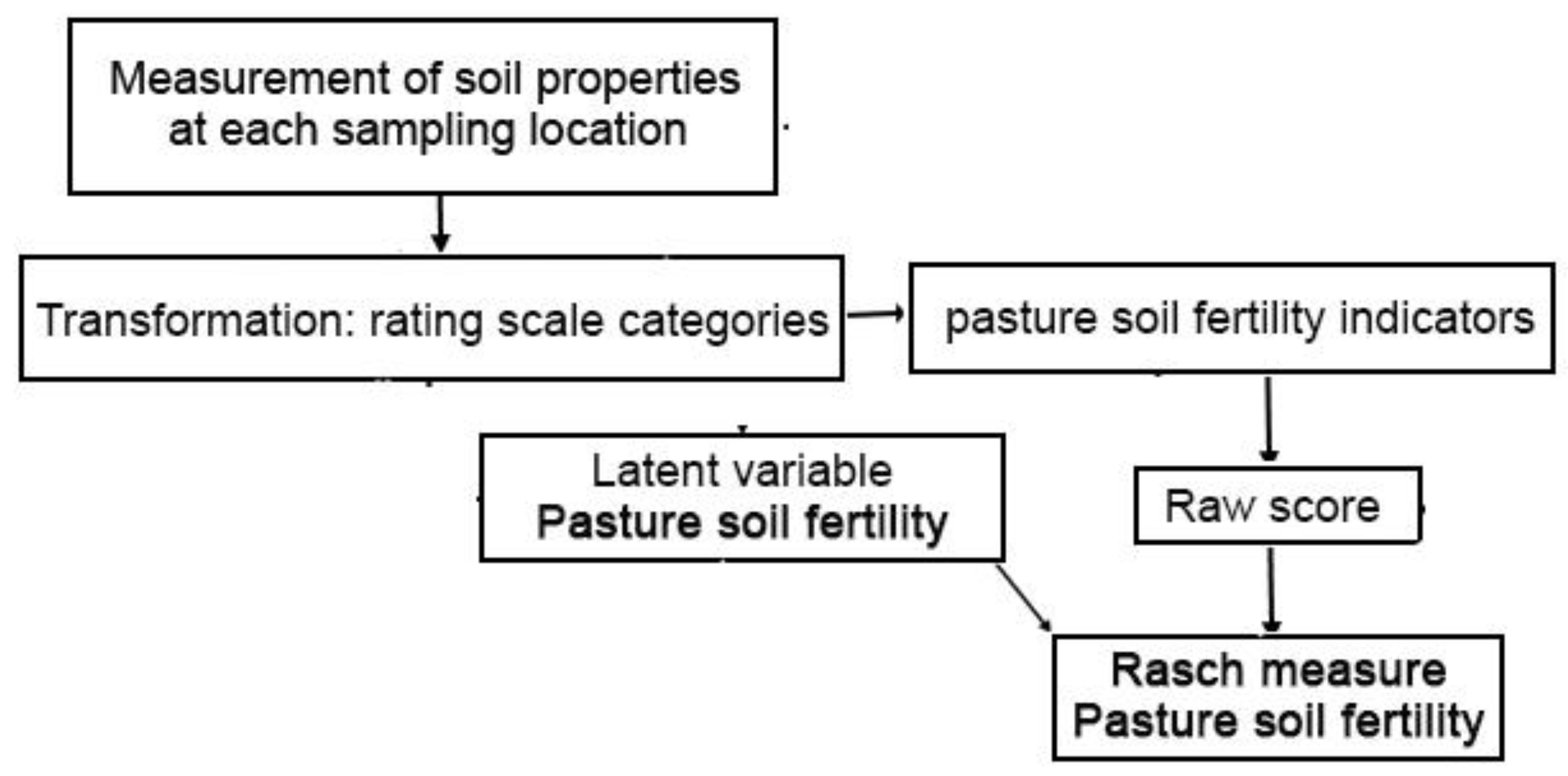
The Winsteps v. 4.0 computer program [35] was used to implement the Rasch model. More information about its mathematical formulation can be obtained, for instance, in Tristán [25] and Ferrari and Salini [32]. The stages to formulate the Rasch model are shown in Figure 2. The values of all the soil properties at each sample were measured after considering the locations and the soil properties which are influencing the pasture soil fertility. Then, these data were computed, obtaining the Rasch measures and some statistics to estimate how the fit was.

3. Results and Discussion

Many outputs were obtained after the processing of the matrix for the categorical values. The first step was the overall analysis of the data response to the Rasch model [36]. Table 2 shows the mean raw score (the sum of points of the common scale) and the mean Rasch measure. The mean infit and outfit MNSQ values were very close to 1, the expected value, and the mean standardised (ZSTD) infit and outfit values were close to 0, the expected value, particularly for the sampling locations (Table 2). As the standard deviations of the infit MNSQ for the sampling locations and soil properties are lower than two (Table 2), the possible misfits (the sampling locations or soil properties differing from expectation) are unimportant [37]. In consequence, the items properly fit the model. It is important to indicate how the misfits denote the individual items from the set that do not perform as expected, and the outfit is a single value which refers to the global response of the items, being a standard fit statistic which is highly influenced by a few outliers.
The raw score (the sum of the points of all the categories for each property) at each sampling location and the measured values, obtained from the raw scores with the Winsteps programme, are shown in Table 3. The sampling locations are from the highest to the lowest soil fertility, i.e., in measure order. The most fertile locations are all from Cubillos; the second field with the most fertile locations is Grous. The rest of the fields have locations with a high and low soil fertility, that is, their spatial variability is more important. This is related to the predominant soil texture in each field. The mean sand content in Cubillos and Grous is 37.5% and 57.6%, respectively, while it is higher than 70% in the other five fields. Moreover, the mean clay content in Cubillos is 23.5%, in Grous is 16.8% and it is lower than 10% in the other fields [14]. Some previous studies in agricultural fields where the clay contents were higher showed their influence on the soil fertility [23,38].
After analysing the misfits, i.e., the sampling locations which do not follow the pattern of the model, it was found that a low amount of them (only five soil samples) had at least one misfit, accounting for approximately 12% of the samples. The sampling locations that displayed a misfit are shown in Table 4. Two samples had two misfits. When the residuals were positive, the score for the sample in those residuals was higher than expected. Negative residuals indicate that the score was lower than expected. Thus, the sample AZI01 has a low fertility (−1.08) but the organic matter content is too high and the score is, in turn, the maximum, five. We expected to have a lower organic matter content in this sampling location. Unlike the previous sample, the sampling location GRO11 has a high fertility (0.52) but the score is too low, at one. A higher organic matter content would be expected in this sampling location. Moreover, the expected slope was lower than the existing in this place. Similar explanations can be argued for the other misfits in each sample and soil property shown in Table 4.
Table 5 shows the relative influence of each soil property on the latent variable, the pasture fertility, being the raw score the sum of the points of the common scale for each soil property considering all the samples (42) and the measure the position of each soil property along the straight line that represents the latent variable, the soil fertility potential. As it is showed later in Figure 3, the soil properties are in the lower part of the straight line that represents the latent variable, so a highest score corresponds to a lower measure and vice versa [25]. Thus, the slope is the property exerting the highest influence on the pasture soil fertility in these fields. It has the highest raw score (and the lowest measure). This is because this topographical variable determines the level of the other soil properties, for instance, the textural components [39]. In contrast, the clay content has the lowest overall influence on the soil fertility in these fields, with the lowest raw score (and the highest measure). The sand content has also a low influence on the soil fertility. In consequence, as it could be expected, the textural components are not globally important in these sandy fields to define the most fertile zones, except for those fields, Cubillos and Grous, where the clay content is higher, with a mean value of 23.5% and 16.8%, respectively [14] However, the low clay content in the other five fields, with a mean value lower than 9%, makes this soil property, as previously indicated, be the one less influential on the overall soil fertility considering all the experimental fields. In fact, the fertility level at each sampling location in any field is related to the clay content because the moisture and nutrient contents in the locations with a higher clay content are also higher [5]. In the sandy soils, water drains very quickly and washes away most of the nutrients.
Figure 3 shows the soil properties and the sampling locations in the same scale, according to the pasture soil fertility, in the upper and lower half of the diagram. Above the line, the distribution of soil samples is shown: to the left, those are less fertile and to the right, those are more fertile. Below the line, the soil properties are distributed: to the left are the more common (frequent) properties, with a higher influence on the pasture soil fertility, and to the right are the less common (rare) properties, with a lower influence on the pasture soil fertility. As previously indicated, the clay content is more to the right in the straight line, that is, it is the soil property with the highest measure. K2O is close to the clay content and the other properties are located to the left, that is, they have lower measures. The slope is the property with the lowest measure, with it being more to the left.
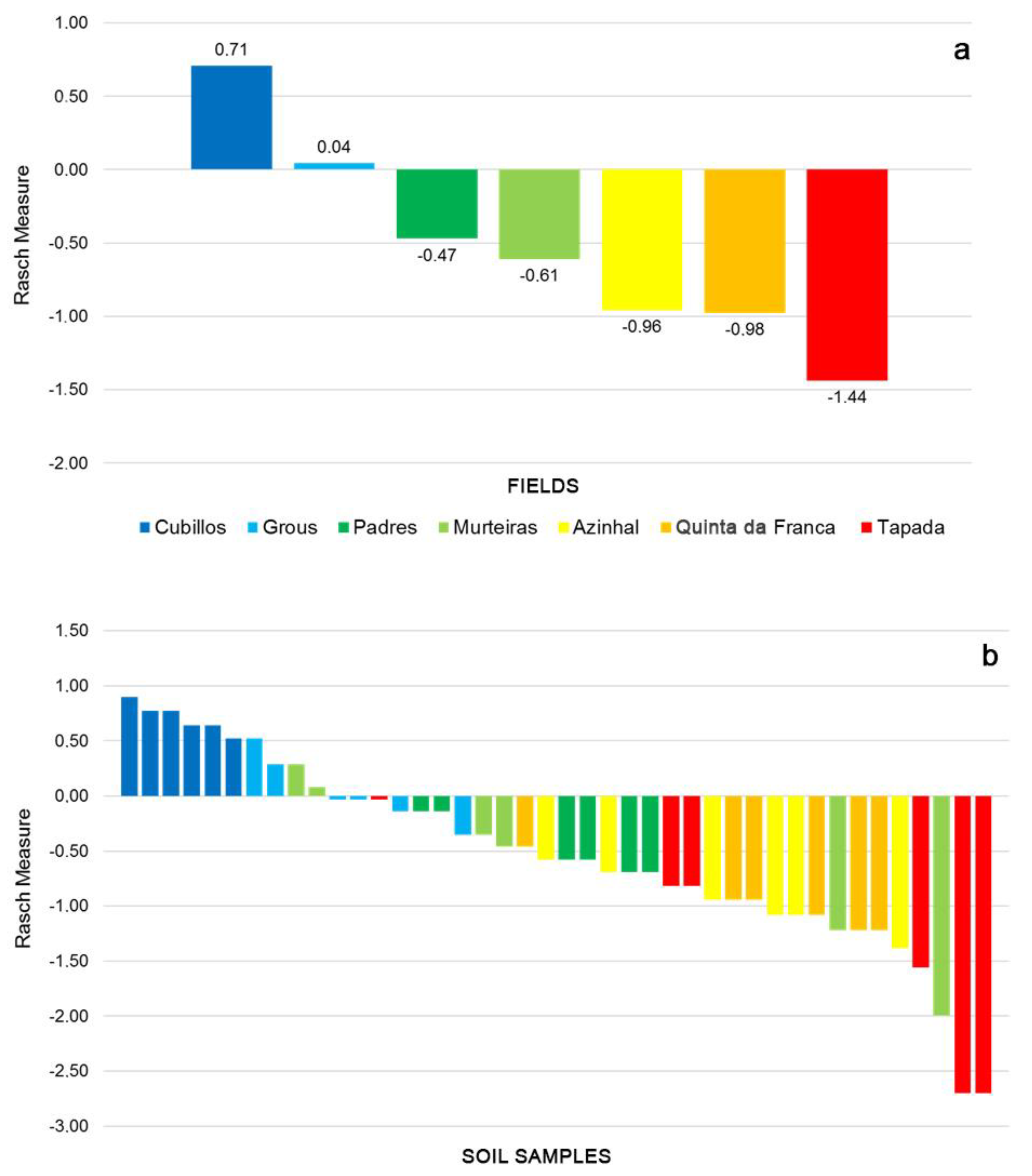
With respect to the distribution of the sampling locations in the continuum (Figure 3), most of them have a low pasture soil fertility because their score is very low. However, a high intra and inter field variability exists. Figure 4 shows the soil pasture fertility in each field according to the Rasch measure. The differences between the mean value of the Rasch measure in Cubillos are apparent, where there is a high soil fertility. In contrast, Tapada has a very low soil fertility, with the lowest mean Rasch measure. Considering all the sampling locations of each field (Figure 4), the sampling locations are aggregated only in Cubillos (they are at the right of the continuum in Figure 3), with a high fertility level. In the rest of the fields, the sampling locations have more variability (they are situated along the straight line in Figure 3), but the fields where the sampling locations are less fertile are situated in Tapada, Quinta da França and Azinhal (Figure 4). Almost half of the sampling locations, 20, reached 23 points in the raw score, more than half of the maximum (45 points). This indicates that at many locations, the soil fertility is not optimum. Moreover, the mean Rasch measure for the samples is more to the left than the mean Rasch measure for the soil properties (Figure 3), which is an additional indication about the overall low soil fertility.
The existence of important differences within each field makes them suitable for a site-specific management [14]. In consequence, the overall potential for the pasture yield in the fields is very different according to their soil pasture fertility and, moreover, there is an important spatial variability between the zones within each field, even though these fields are not generally very fertile. Serrano et al. [14] reported similar results in a previous study using another methodology.

4. Conclusions

The results of this study show that the formulation of the Rasch model, integrating the most significant soil variables, can be used to analyse the differences in the pasture soil fertility between fields. Topography, particularly the slope, was the main factor affecting the pasture soil fertility in the analysed fields and the textural components of the soils are not globally important. Despite the fact that the clay content is very influential at the local sites, determining its spatial differences, its level is very low in most of the considered fields.
It was obtained that two of the experimental fields, Cubillos and Grous, have a higher overall soil fertility. Moreover, the within-field variability in the pasture soil fertility was also highlighted as the differences in the Rasch measures at different sampling locations.
In consequence, the proposed method is an objective way to improve the efficiency of the use of inputs by adjusting them to the pasture and soil variability. This information can be completed with the analysis of different places within each field, as a rational way to study the variability that is usual in soil fertility. Later, more in-depth studies can be conducted in each field to delineate the MZ where site-specific management is recommended to optimise the application of the inputs and a more cost-effective field management, in addition to the energy and environmental benefits.

Author Contributions

Conceptualization, F.J.M. and J.M.S.; methodology, F.J.M., J.M.S. and F.J.R.; software, F.J.M. and F.J.R.; validation, F.J.M. and F.J.R.; formal analysis, F.J.M. and J.M.S.; investigation, F.J.M., J.M.S. and T.D.; resources, J.M.S., R.F.M.T. and T.D.; data curation, F.J.M. and F.J.R.; writing—original draft preparation, F.J.M.; writing—review and editing, F.J.M., J.M.S., R.F.M.T. and T.D.; visualization, F.J.R.; supervision, F.J.M. and J.M.S.; project administration, J.M.S., R.F.M.T. and T.D.; funding acquisition, F.J.M., J.M.S., R.F.M.T. and T.D. All authors have read and agreed to the published version of the manuscript.

Funding

This research was funded by the Junta de Extremadura and the European Regional Development Fund (ERDF) through the Project GR21006 (Research Group TIC008), by Portuguese Funds through FCT (Foundation for Science and Technology) under Projects UIDB/05183/2020 and CEECIND/00365/2018 (R. Teixeira), by FCT/MCTES (PIDDAC) through project UID/EEA/50009/2019, and by the projects PDR2020-101-030693 and PDR2020-101-031244 (“Programa 1.0.1-Grupos Operacionais”).

Data Availability Statement

The data presented in this study are available on request from the corresponding author. The data are not publicly available due to confidentiality reasons.

Conflicts of Interest

The authors declare no conflict of interest. The funders had no role in the design of the study; in the collection, analyses, or interpretation of data; in the writing of the manuscript, or in the decision to publish the results.

References

  1. David, T.S.; Henriques, M.O.; Kurz-Besson, C.; Nunes, J.; Valente, F.; Vaz, M.; Pereira, J.S.; Siegwolf, R.; Chaves, M.M.; Gazarini, L.C.; et al. Water-use strategies in two co-occurring Mediterranean evergreen oaks: Surviving the summer drought. Tree Physiol. 2007, 27, 793–803. [Google Scholar] [CrossRef] [PubMed] [Green Version]
  2. Nawar, S.; Corstanje, R.; Halcro, G.; Mulla, D.; Mouaze, A.M. Chapter dour-delineation of soil management zones for variable-rate fertilization: A review. Adv. Agron. 2017, 143, 175–245. [Google Scholar]
  3. Moral, F.J.; Rebollo, F.J.; Serrano, J.M. Delineating site-specifc management zones on pasture soil using a probabilistic and objective model and geostatistical techniques. Precis. Agric. 2020, 21, 620–636. [Google Scholar] [CrossRef]
  4. Serrano, J.; Shahidian, S.; Marques da Silva, J.; Paixao, L.; Calado, J.; de Carvalho, M. Integration of soil electrical conductivity and indices obtained through satellite imagery for differential management of pasture fertilization. AgriEngineering 2019, 1, 567–585. [Google Scholar] [CrossRef] [Green Version]
  5. Moral, F.J.; Rebollo, F.J.; Serrano, J.M.; Carvajal, F. Mapping management zones in a sandy pasture soil using an objective model and multivariate techniques. Precis. Agric. 2021, 21, 620–636. [Google Scholar] [CrossRef]
  6. Serrano, J.; Shahidian, S.; Marques da Silva, J.; Sales-Baptista, E.; Ferraz de Oliveira, I.; Lopes de Castro, J.; Pereira, A.; Cancela d’Abreu, M.; Machado, E.; Carvalho, M. Tree influence on soil and pasture: Contribution of proximal sensing to pasture productivity and quality estimation in montado ecosystems. Int. J. Remote Sens. 2018, 39, 4801–4829. [Google Scholar] [CrossRef]
  7. Schellberg, J.; Hill, M.J.; Roland, G.; Rothmund, M.; Braun, M. Precision agriculture on grassland: Applications, perspectives and constraints. Eur. J. Agron. 2008, 29, 59–71. [Google Scholar] [CrossRef]
  8. Diffenbaugh, N.S.; Giorgi, F. Climate Change Hotspots in the CMIP5 Global Climate Model Ensemble. Clim. Chang. 2012, 114, 813–822. [Google Scholar] [CrossRef] [Green Version]
  9. Peralta, N.R.; Costa, J.L.; Balzarin, M.; Franco, M.C.; Córdoba, M.; Bullock, D. Delineation of management zones to improvenitrogen management of wheat. Comput. Electron. Agric. 2015, 110, 103–113. [Google Scholar] [CrossRef]
  10. Moral, F.J.; Rebollo, F.J.; Serrano, J.M. Estimating and mapping pasture soil fertility in a portuguese montado based on a objective model and geostatistical techniques. Comput. Electron. Agric. 2019, 157, 500–508. [Google Scholar] [CrossRef]
  11. Moral, F.J.; Serrano, J.M. Using low-cost geophysical survey to map soil properties and delineate management zones on grazed permanent pastures. Precis. Agric. 2019, 20, 1000–1014. [Google Scholar] [CrossRef]
  12. Serrano, J.; Peça, J.; Marques da Silva, J.; Shahidian, S. Mapping soil and pasture variability with an electromagnetic induction sensor. Comput. Electron. Agric. 2010, 73, 7–16. [Google Scholar] [CrossRef]
  13. Stefanski, A.; Simpson, R.J. Uneven nurient distributionin hillside paddocks indicate potential need for variable rate fertiliser application to pastures. In Food Security from Sustainable Agriculture, Proceedings of the 15th Australian Agronomy Conference, Lincoln, New Zealand, 15–18 November 2010; Dove, H., Culvenor, R., Eds.; Australian Society of Agronomy/The Regional Institute Ltd.: Gosford, NSW, Australia, 2010. [Google Scholar]
  14. Serrano, J.; Shahidian, S.; Paixão, L.; Marques da Silva, J.; Moral, F. Management Zones in Pastures Based on Soil Apparent Electrical Conductivity and Altitude: NDVI, Soil and Biomass Sampling Validation. Agronomy 2022, 12, 778. [Google Scholar] [CrossRef]
  15. Shaddad, S.M.; Madrau, S.; Castrignanò, A.; Mouazen, A.M. Data fusion techniques for delineation of site-specific management zones in a field in UK. Precis. Agric. 2016, 17, 200–217. [Google Scholar] [CrossRef]
  16. Gavioli, A.; Souza, E.G.; Bazzi, C.L.; Guedes, L.P.C.; Schenatto, K. Optimization of management zone delineation by using spatial principal components. Comput. Electron. Agric. 2016, 127, 302–310. [Google Scholar] [CrossRef]
  17. Fortes, R.; Millán, S.; Prieto, M.H.; Campillo, C. A methodology based on apparent electrical conductivity and guided soil samples to improve irrigation zoning. Precis. Agric. 2015, 16, 441–454. [Google Scholar] [CrossRef]
  18. Trotter, M.; Guppy, C.; Haling, R.; Trotter, T.; Edwards, C.; Lamb, D. Spatial variability in pH and key soil nutrients: Is this an opportunity to increase fertiliser and lime-use efficiency in grazing systems? Crop Pasture Sci. 2014, 65, 817–827. [Google Scholar] [CrossRef]
  19. Xin-Zhong, W.; Guo-Shun, L.; Hong-Chao, H.; Zhen-Hai, W.; Qing-Hua, L.; Xu-Feng, L.; Wei-Hong, H.; Yan-Tao, L. Determination of management zones for a tobacco field based on soil fertility. Comput. Electron. Agric. 2009, 65, 168–175. [Google Scholar] [CrossRef]
  20. Ortega, R.A.; Santibáñez, O.A. Determination of management zones in corn (Zea mays L.) based on soil fertility. Comput. Electron. Agric. 2007, 58, 49–59. [Google Scholar] [CrossRef]
  21. Li, Y.; Shi, Z.; Li, F.; Li, H.Y. Delineation of site-specific management zones using fuzzy clustering analysis in a coastal saline land. Comput. Electron. Agric. 2007, 56, 174–186. [Google Scholar] [CrossRef]
  22. Morari, F.; Castrignanò, A.; Pagliarin, C. Application of multivariate geostatistics in delineating management zones within a gravelly vineyard using geo-electrical sensors. Comput. Electron. Agric. 2009, 68, 97–107. [Google Scholar] [CrossRef]
  23. Moral, F.J.; Terrón, J.M.; Rebollo, F.J. Site-specific management zones based on the Rasch model and geostatistical techniques. Comput. Electron. Agric. 2011, 75, 223–230. [Google Scholar] [CrossRef]
  24. Rebollo, F.J.; Moral, F.J.; Campillo, C.; Marques da Silva, J.R.; Serrano, J.M.; Pérez-Rodríguez, J.M. Delineation of management zones based on the Rasch model in an olive orchard. In Proceedings of the 11th European Conference on Precision Agriculture, Edinburgh, UK, 16–20 July 2017. [Google Scholar]
  25. Tristán, A. Análisis De Rasch Para Todos; Ceneval: Mexico City, Mexico, 2002. [Google Scholar]
  26. FAO. World reference base for soil resources. In World Soil Resources Reports N. 103; Food and Agriculture Organization of the United Nations: Rome, Italy, 2006. [Google Scholar]
  27. Peel, M.C.; Finlayson, B.L.; McMahon, T.A. Updated world map of the Köppen-Geiger climate classification. Hydrol. Earth Syst. Sci. 2007, 11, 1633–1644. [Google Scholar] [CrossRef] [Green Version]
  28. Egner, H.; Riehm, H.; Domingo, W.R. Utersuchungeniiber die chemische Bodenanalyse als Grudlagefir die Beurteilung des Nahrstof-zunstandes der Boden. II. K. Lantbr. Ann. 1960, 20, 199–216. [Google Scholar]
  29. Hambleton, R.K.; Swaminathan, H.; Rogers, H.J. Fundamentals of Item Response Theory; Sage Publishing: Newbury Park, CA, USA, 1991. [Google Scholar]
  30. Álvarez, P. Transforming non categorical data for Rasch analysis. In Rasch Measurement in Health Sciences; JAM Press: Maple Grove, MN, USA, 2004. [Google Scholar]
  31. Rasch, G. Probabilistic Models for Some Intelligence and Attainment Tests; Revised and expanded ed.; University of Chicago Press: Chicago, IL, USA, 1980. [Google Scholar]
  32. Ferrari, P.A.; Salini, S. Complementary use of Rasch Models and Nonlinear Principal Component Analysis in the Assessment of the Opinion of European About Utilities. J. Classif. 2011, 28, 53–69. [Google Scholar] [CrossRef]
  33. Bond, T.G.; Fox, C.M. Applying the Rasch Model: Fundamental Measurement in the Human Sciences; Lawrence Erlbaum Associates Inc.: Mahwah, NJ, USA, 2007. [Google Scholar]
  34. Edwards, A.; Alcock, L. Using Rasch analysis to identify uncharacteristic responses to undergraduate assessments. Teach. Math. Its Appl. Int. J. IMA 2010, 29, 165–175. [Google Scholar] [CrossRef] [Green Version]
  35. Linacre, J.M. Winsteps (Computer Program and Manual); MESA Press: Chicago, IL, USA, 2009. [Google Scholar]
  36. Sekaran, U. Research Methods for Business: A Skill Building Approach; John Wiley & Sons Ltd.: New York, NY, USA, 2000. [Google Scholar]
  37. Bode, R.K.; Wright, B.D. Rasch measurement in higher education. In Higher Education: Handbook of Theory and Research; Smart, J.C., Tierney, W.G., Eds.; Agathon Press: New York, NY, USA, 1999. [Google Scholar]
  38. Moral, F.J.; Rebollo, F.J. Characterization of soil fertility using the Rasch model. J. Soil Sci. Plant Nutr. 2017, 17, 486–498. [Google Scholar] [CrossRef]
  39. Ceddia, M.B.; Vieira, S.R.; Villela, A.L.O.; Mota, L.S.; Anjos, L.H.C.; Carvalho, D.F. Topography and spatial variability of soil physical properties. Sci. Agric. 2009, 66, 338–352. [Google Scholar] [CrossRef]
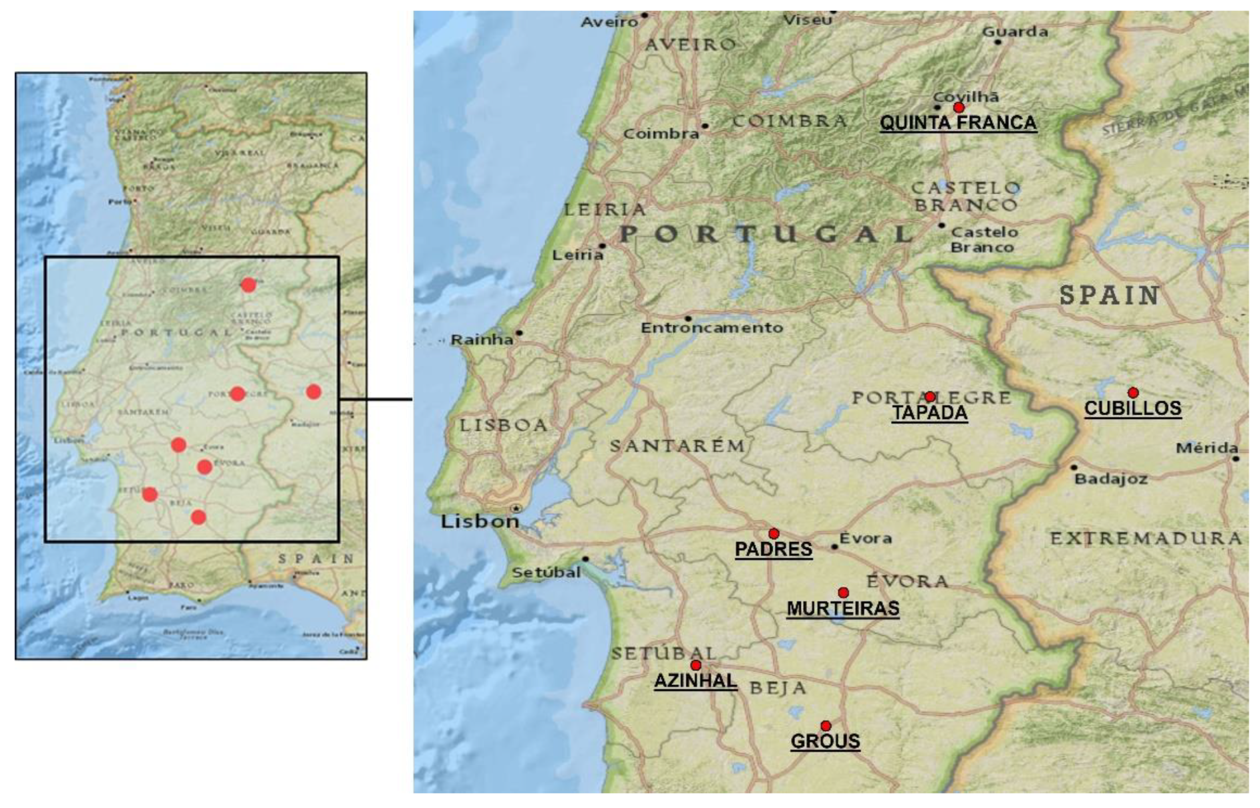
Figure 1. Location of the seven experimental fields.
Agronomy 12 02711 g001
Figure 2. Formulation of the Rasch model.
Agronomy 12 02711 g002
Figure 3. Straight line representing the latent variable: pasture soil fertility. The mean values of the Rasch measure for soil samples and properties are ms and mp, respectively (Azinhal—AZI, Padres—PAD; Tapada—TAP; Cubillos—CUB; Grous—GRO; Murteiras—MUR, and Quinta da França—QF).
Agronomy 12 02711 g003
Figure 4. (a) Rasch measure (mean value of the soil fertility) in each experimental field. (b) Rasch measure (soil fertility) at each sampling location of all experimental fields.
Agronomy 12 02711 g004
Table 1. Experimental fields in this study.
FieldCoordinatesArea (ha)Soil TexturePredominant TreesAnimal Species (Type of Grazing)
Quinta da França40°16.78′ N; 7°25.34′ W25.3Loamy sandOaks and eucalyptusHorses, cattle and sheep (rotational grazing)
Azinhal38°6.2′ N; 6°44.6′ W22.3Sandy loamHolm and cork oakSheep (rotational grazing)
Cubillos39°10′ N; 6°44.6′ W32.8LoamHolm and cork oakCattle and pigs (rotational grazing)
Grous37°52.3′ N; 7°56.7′ W28.3Sandy loamHolm oakCattle (rotational grazing)
Murteiras38°23.4′ N; 7°52.5′ W29.6Sandy loamHolm oakSheep (permanent grazing)
Padres38°36.4′ N; 8°8.7′ W32.2Loamy sandHolm oakCattle (permanent grazing)
Tapada39°9.5′ N; 7°31.9′ W27.1Loamy sandHolm and cork oakCattle and pigs (rotational grazing)
Table 2. Summary of all 9 soil properties and all 42 soil samples. Overall model fit information.
InfitOutfit
Raw ScoreMeasureMNSQZSTDMNSQZSTD
Mean23.1−0.530.97−0.050.990.02
Standard Deviation6.50.850.521.020.540.99
Maximum350.902.662.962.843.12
Minimum11−2.700.31−1.810.38−1.33
Summary soil samples
Mean107.90.001.01−0.20.99−0.29
Standard Deviation25.30.660.462.090.471.93
Maximum1530.791.883.181.862.6
Minimum79−1.170.48−3.160.45−3.02
Summary soil properties
Table 3. Results for sampling locations, after the formulation of the Rasch model.
Sampling LocationRaw ScoreMeasure
CUB 13350.90
CUB 06340.77
CUB 01340.77
CUB 14330.64
CUB 05330.64
CUB 09320.52
GRO 11320.52
GRO 07300.29
MUR 04300.29
QF B0618−1.08
MUR 0717−1.22
QF B0117−1.22
QF A0417−1.22
AZI 1516−1.38
TAP 0115−1.56
MUR 0913−2.00
TAP 0511−2.70
TAP 1511−2.70
Only some sampling points are shown. In total there are 42 samples from seven fields (Azinhal—AZI, Padres—PAD; Tapada—TAP; Cubillos—CUB; Grous—GRO; Murteiras—MUR, and Quinta da França—QF).
Table 4. Soil samples where misfits have been computed.
K2OTNOMCECECSlopeSample
Score: 5 AZI01
Misfit: 4
Score: 5 AZI15
Misfit: 3
Score:51 GRO19
Misfit:3−2
Score: 1 3GRO11
Misfit: −2 −2
Score: 5 GRO07
Misfit: 2
Table 5. Results for soil properties, after the formulation of the Rasch model.
ItemRaw ScoreMeasureInfit MNSQInfit ZSTDOutfit MNSQOutfit ZSTD
Clay790.790.91−0.320.81−0.62
K2O810.731.883.181.862.60
Sand900.450.87−0.540.76−0.98
ECa950.311.622.551.612.23
TN1040.080.48−3.160.45−3.02
Silt112−0.130.55−2.690.51−2.76
CEC120−0.321.020.191.050.31
OM137−0.740.81−0.930.85−0.68
Slope153−1.170.97−0.051.060.32
Publisher’s Note: MDPI stays neutral with regard to jurisdictional claims in published maps and institutional affiliations.