Article

The Dynamic Impacts of Weather Changes on Vegetable Price Fluctuations in Shandong Province, China: An Analysis Based on VAR and TVP-VAR Models

College of Public Administration, Huazhong Agricultural University, Wuhan 430070, China
*
Author to whom correspondence should be addressed.
Agronomy 2022, 12(11), 2680; https://doi.org/10.3390/agronomy12112680
Submission received: 2 September 2022 / Revised: 8 October 2022 / Accepted: 24 October 2022 / Published: 28 October 2022

Abstract

:
In order to enrich the research on the influence of weather factors on agricultural economy and provide practical decision-making references for the relevant market entities, this study took pointed pepper, loofah, Chinese chives and tomato as examples, using weekly wholesale prices and corresponding weather factors data from one of the main production areas in China based on the vector autoregressive (VAR) and the time-varying parameter vector autoregressive (TVP-VAR) models to explore the dynamic impacts of weather changes on vegetable price fluctuations. It was found that price fluctuations of specific vegetable varieties were affected by changes in specific weather factors. The shock intensity of weather factor changes in the same lag period on the current vegetable price fluctuations was time-varying, which could describe the historical dynamics of the impacts of weather changes on vegetable price fluctuations. The dissipation characteristics of the dynamic impacts of weather factors changes occurring at selected time points on vegetable price fluctuations had strong consistency, and the obtained rules could be used to analyze the life cycle and dynamic characteristics of extreme weather impacts on vegetable price fluctuations. In addition, vegetable price fluctuations were affected mostly by their own lag periods, and the shock intensity of vegetable price fluctuations with equal lag periods on their own current price fluctuations were relatively stable. The dynamic impacts of vegetable price fluctuations occurring at chosen time points on its own later fluctuations were highly consistent in the variation from the beginning of the strongest positive shock to the final dissipation.

1. Introduction

China is the world’s largest producer and consumer of vegetables, and vegetables are indispensable in people’s daily diet and are an important guarantee of their quality of life [1]. The positive development of the vegetable industry and smooth operation of the vegetable market is related to people’s livelihood, vegetable price fluctuations involving the vital interests of many subjects. In reality, abnormal fluctuations in vegetable prices occur frequently, seriously affecting the economic interests of producers, business operators and consumers. The internal and external causes of abnormal fluctuations in vegetable prices are complex and varied, among which weather changes can affect the whole process of vegetable planting, harvesting, transportation and selling to varying degrees and impact vegetable market prices through market supply and demand mechanisms [2,3,4]. The spatial concentration of vegetable production and the dispersed consumer market in China make the vegetable supply chain more susceptible to extreme weather, causing imbalances in supply and demand in the vegetable market and thus leading to abnormal fluctuations in vegetable prices on a large scale, affecting people’s livelihoods [5]. Therefore, the study of the dynamic impacts of weather changes in the main production areas on vegetable price fluctuations is of great theoretical and practical significance in China.
The main contributions of this study are: (1) Explicitly established a direct link between weather factors and vegetable prices, skipping the study of the impact of weather factors on vegetable yield and quality. (2) The data for the study came from one of the main vegetable production areas of a large vegetable-producing and consuming country, so the findings of the study were more representative and referential. (3) Empirically demonstrated that there was an impact of weather changes on vegetable price fluctuations and could indicate which specific weather factors affected particular vegetable varieties and what was the proportion of the contribution of each weather factor in price fluctuations. (4) Empirically demonstrated the time-varying effects of weather changes on vegetable price fluctuations and derived a dynamic response mechanism for the price fluctuations of specific varieties of vegetables to specific weather factors. (5) Derived the dynamic response of vegetable price fluctuations after weather changes at any point in time, especially when extreme weather occurs. (6) Empirically proved the dynamic response mechanism of vegetable price fluctuations to their own lag periods. This study extended the research on the impact of weather changes on vegetable price fluctuations; provided a theoretical reference for vegetable price forecasting and early warning research and provided a decision reference for government policies, as well as practical behaviors of related farmers, businessmen and consumers.
The remainder of the paper is organized as follows. Section 2 reviews related studies. Section 3 presents the overall design of this study. Section 4 conducts the analysis and discussion of the empirical results. Section 5 gives the study summary and suggestions.

2. Literature Review

The results of research on the impact of climate and weather on the agricultural economy are relatively abundant. Agriculture is one of the economic sectors mainly affected by climatic and weather factors, especially for countries with large territories [6,7,8]. Due to global climate change, extreme weather is expected to continue to worsen in the coming decades, destabilizing agricultural production systems [9,10,11,12,13,14]. Furuya et al. [15] explored the impacts of climate change on world food markets, which showed that rising temperatures would have remarkable influences on crop production, and the yield variations due to temperature changes were very different for different crops in different countries or regions. Wang et al. [16] used data from China to analyze the impacts of weather factors on net crop incomes, showing that world warming might be detrimental to rainfed farms but really helpful to irrigated farms; the damage to net crop incomes has increased over time, and its impact varies by region. Using corn yield data from the United States, Seo [17] explained the difference between the effects of stochastic weather, which were considered random, and the effects of climate change, which were considered nonrandom, and noting that they had different impacts on agricultural decision-making and were critical for modeling agricultural decisions. Cogato et al. [18] explored the relationship between extreme weather and agriculture through a bibliometric analysis. Research showed that food safety and economic loss from extreme weather events were an important issue, and future research should focus on developing countries responses and governance systems for this issue. Dalhaus et al. [19] concluded that weather factors affected not only crop yields but also the quality of agricultural products and that weather factors were one of the drivers of agricultural income fluctuations and empirically demonstrated the effect of extreme weather on the apple quality. Cui et al. [20] empirically proved the impacts of climate change on agricultural economy, showing that, on average, climate change would decrease yields and raise prices and that climate change had led to an increased uncertainty in forecasting agricultural economies. Increasing climate change enhanced the risk on agricultural production and prices, and the design and implementation of weather-based agricultural insurance has become more important in response to sudden weather disasters, especially in developing countries [21,22,23,24].
Regarding research on the impact of weather changes on agricultural prices, some scholars have empirically demonstrated Granger causality between weather anomalies and agricultural futures prices and that global temperature anomalies affect people’s expectations of agricultural economic activities [25]. Cao et al. [26] found that there was a correlation between weather and agricultural future markets on a certain time scale; under extreme weather conditions, weather had different effects on different agricultural commodities. Letta et al. [27] empirically assessed the impact of abnormal weather in India on traders’ expectations and agricultural market prices, finding that the drought increased the preharvest prices of agricultural products and the expectations channel played an important role in price fluctuations. Pustil Nik et al. [28] described a model of the impact of weather on agricultural markets and proved that space weather had a significant impact on agricultural prices under certain spatial and temporal conditions. Brown et al. [29] quantitatively studied the short-term impacts of local weather and international price disturbances on local agricultural prices, and the results showed that, for most developing countries, local agricultural prices were much more affected by local weather changes than by international agricultural market price fluctuations.
Research on climate change or weather factors and vegetables has mainly focused on studies of the effects of climate or weather variables on vegetable cultivation, yield and quality (involving preharvest and post-harvest vegetable quality) [30,31,32]. Bisbis et al. [33] conducted a literature review of research on the impacts of climate change on vegetable production, physiological responses, yield and product quality, where weather factors were involved such as temperature and precipitation. The influence of climate and weather variables on vegetable prices were mentioned in different degrees in some of this kind of research [30,33]. In addition, some scholars who do research on vegetable price forecasting add weather variables as one kind of the input characteristics in the study, which was based on the assumption that weather factors had an impact on vegetable prices, and the accuracy of vegetable price forecasting could be improved by including weather factors [34,35,36,37]. Nalwanga et al. [38] constructed a vegetable price prediction model based on fuzzy logic and empirically found that it was possible to predict expected tomato production and prices in Kenya using historical data of monthly temperature, humidity and precipitation.
It is clear from the above studies that climate and weather have a significant impact on agricultural production and economy, which is the consensus of academia, and this impact will tend to intensify in the future with the chain reaction of global climate change. Research on climate and weather variables and agricultural prices can be divided into two main areas: the effect on agricultural future prices and on market prices. Although the research on climate or weather and vegetables mainly focuses on the influence of climate change and weather factors on vegetable production and its yield and quality, the influence of climate and weather on vegetable prices has also been explored to some extent, and some scholars have included weather factors in the research on vegetable price predictions to improve the prediction accuracy of their models. In conclusion, the existing research results provide a sufficient theoretical basis for the basic hypothesis of this study: that is, weather changes have impacts on vegetable price fluctuations. Considering the dynamic nature of climate and weather changes and the time delay and historical variability of the feedback of the vegetable market to the exogenous impacts (weather changes), we further proposed the hypothesis that the impacts of weather changes on vegetable price fluctuations are dynamic. We expected to empirically analyze the dynamic impact mechanism of weather changes on vegetable price fluctuations under specific spatial and temporal conditions and draw some specific, exact results and general conclusions, so as to expand and deepen the research on the impacts of weather changes on vegetable price fluctuations.
Based on the above analysis, hypotheses and expectations, this paper empirically analyzed the dynamic impacts of weather changes on vegetable price fluctuations. Pointed pepper, loofah, Chinese chives and tomato were selected as representatives of the vegetable varieties, and the temperature, precipitation, relative humidity and sunshine duration were selected as representatives of the weather factors. The Granger causality test [39] was used to verify the causal relationship between weather factors and vegetable prices; the variance decomposition function of the vector autoregressive (VAR) model [40] was used to explore the contribution weight of different weather factors to vegetable price fluctuations and the impulse response analysis function of the time-varying parameter vector autoregressive (TVP-VAR) model [41] was used to empirically test the time-varying impulse response mechanism of the price fluctuations of specific vegetable varieties to changes in specific weather factors.

3. Methodology and Data

3.1. Research Framework

This study was conducted according to the experimental procedure shown in Figure 1, which was divided into three major parts: data preprocessing; construction of a VAR model for variance decomposition analyses and construction of a TVP-VAR model for impulse response analyses. Firstly, the vegetable prices and weather factors time series data were subjected to first-order differencing, and the processed data reflected the volatility of the variables. The data were then tested by unit root to ensure the stationarity of the time series. Based on the unit root test, a vegetable price and weather factors were used to construct the VAR model, and then, the optimal lag order was selected according to the Akaike information criterion (AIC) [42] and the final prediction error (FPE) criterion [43,44]. The optimal lag order was used to carry out the Granger causality test of the price and weather factors, and the weather factors through the Granger causality test were selected as the Granger cause of vegetable price fluctuation. Then, the selected weather factors and prices were used to construct the VAR model again, so as to cycle until the stable optimal lag order could be obtained. Under this optimal lag order condition, the selected weather factors were all the Granger causes of vegetable price fluctuation. The VAR model was constructed using the final selected optimal lag order and variables, and a variance decomposition analysis was performed under the premise that the VAR model was stable. Finally, the TVP-VAR model was constructed using the same optimal lag order and variables, and the impulse response analysis of the equal interval and the impulse response analysis at different time points could be performed after passing the model estimation and parameter testing. Following this experimental procedure, all experiments for the four vegetable varieties were completed.

3.2. Methodology

The vector autoregressive (VAR) model is a commonly used econometric model that was proposed by Christopher Sims in 1980 [40]. The VAR model incorporates different variables into a unified analytical framework and is able to obtain the coefficients of interaction effects while controlling for other variables and is also able to visualize the degree of influence of different variables through variance decomposition. Based on the variance decomposition function of the VAR model, the impact contribution ratio of each weather factor change to the fluctuations of vegetable price could be analyzed. There is an underlying assumption in the VAR model that the estimated coefficients and the variance of the disturbance terms do not change over time. This approach improves the efficiency of the calculations, and the results reflect the overall interaction but have the disadvantage of masking the variability of the shock effects. With the development of time, various external environmental conditions such as economic cycles, policies and regulations and technological innovations may produce huge changes—at which time, the traditional VAR model can no longer be used to portray the changing model parameters. The time-varying parameter vector autoregressive (TVP-VAR) model is a good solution to this problem [41]. The use of the TVP-VAR model enabled the analysis of the dynamic variability of the impact of weather changes on vegetable price fluctuations [45]. According to Primiceri [41] and Nakajima [46], the construction methods of the VAR and TVP-VAR models are shown as follows.
The basic structural VAR model was:
  A y t = F 1 y t 1 + + F s y t s + μ t , t = s + 1 , , n .  
where y t was a k × 1 dimensional vector composed of the observed variables, A, F 1 , ,   F s   were   k × k dimensional coefficient matrixes and the perturbation term μ t denoted k × 1   dimensional structural shock. μ t was assumed to obey a normal distribution μ t ~ N 0 , , and was satisfied:
= σ 1 0 0 0 0 0 0 σ k
Matrix A was a lower triangular matrix:
A = 1 0 0 α 21 0 α k 1 α k , k 1 0
Equation (1) could be rewritten as:
y t = B 1 y t 1 + + B s y t s + A 1 ε t , ε t ~ N   ( 0 ,   I k )
Among them, B i = A 1 F i , i = 1 , , s . ε t   was defined as an additive shock, which was assumed to be independent of any other innovation. The elements in matrix B i   were expanded into a k 2 s × 1 dimensional vector β by rows and defined X t = I k y t 1 , , y t s ,   as the Kronecker product; then, the model could be rewritten as:
y t = X t β + A 1 ε t
The TVP-VAR model could be obtained by allowing the equation coefficient β , parameter A and covariance matrix ε t in Equation (5) to change with time:
y t = X t β t + A t 1 t ε t t = s + 1 ,   ,   n .
Let α t = α 21 , α 31 , α 32 , α 41 , , α k , k 1 denote the stacked vector of the lower triangular elements in A t . Let   h t = h 1 t , h 2 t , , h k t , where   h j t = log σ j t 2   (j = 1 , 2 , , k ;   t = s + 1 , , n ) [41].
The time-varying parameters in (6) to be estimated followed a random walk process: β t + 1 = β t + μ β t , α t + 1 = α t + μ α t ,   h t + 1 = h t + μ h t , and
  ε t μ β t μ α t μ h t ~ N 0 , I k 0 0 0 0 β 0 0 0 0 α 0 0 0 0 h ,   t = s + 1 ,   ,   n .
Among them, β s + 1 ~ N μ β 0 , β 0 ,   α s + 1 ~ N μ α 0 ,   α 0 ,   h s + 1 ~ N μ h 0 , h 0 . The shocks of time-varying parameters were assumed to be uncorrelated. β ,   α and h were all assumed to be diagonal matrices. The estimation of the parameters of the TVP-VAR model could be done using the Markov Chain Monte Carlo (MCMC) method [47]. The MCMC method is a set of algorithms that sample from a random distribution using a martingale chain. It only requires an artificially set prior probability distribution to be able to estimate the posterior probability distribution of the parameters through circular iterations, and during the iteration process, the posterior probability distribution will gradually approximate the true distribution of the parameters, and the artificially set prior distribution in the model has little effect on the results. In this study, the Markov Chain Monte Carlo (MCMC) algorithm sampling times were set to 10,000, and the first 1000 preheated samples were automatically discarded in order to ensure that the acquired samples did not depend on the initial values and to obtain more robust estimation results [48,49]. The software of MATLAB was used well for this analysis work.

3.3. Data

Data for the study were obtained from Buruike Agricultural Data (https://www.agdata.cn) (accessed on 18 October 2021). Daily weather data and daily wholesale price data were selected from Shandong Province, China, spanning the period from 1 August 2016 to 20 September 2020. Weather data include the daily maximum temperature (degrees Celsius), minimum temperature, average temperature, precipitation (mm), maximum relative humidity (%), minimum relative humidity and sunshine duration (hours). Price data are for four common vegetables in China: pointed pepper, loofah, Chinese chives and tomato. Since the price of fresh and raw vegetables is formed at the wholesale market, the wholesale price of vegetables was chosen as the vegetable price data representative in this study [50]. By checking the Chinese Agricultural Information Network (https://wlw.hx3n.com) (accessed on 16 October 2021), it was known that, in the past few years, Shouguang (Sg) County was one of the main producing areas of pointed pepper and loofah in Shandong Province, and Changle (Cl) County was one of the main producing areas of Chinese chives and tomato in Shandong Province. The wholesale vegetable prices were province-wide averages, and the weather data was county-wide. Considering the vegetable production cycle, vegetable transportation efficiency and vegetable shelf life, weekly data were considered to be a more appropriate frequency for experimental observations in this study, so the frequency of data used in this study was weekly data, with a total of 216 weekly values. The weekly data of wholesale price, temperature and relative humidity were obtained by averaging the daily data in the corresponding time, and the precipitation and sunshine duration were obtained by adding up the daily data.
In this study, the weekly data were further first-order differenced to reflect the volatility of the data, while doing so helped all the time series to pass the unit root test and meet the subsequent modeling conditions. After the first-order difference processing, there are 215 values for each time series. Since weekly data were used in this study, one period represents a week in variance decomposition and impulse response analysis, and one time point represents a certain week within a 215-week period in the time point impulse response analysis.
Table 1 and Table 2 show the results of descriptive statistics for data on prices and weather factors, respectively. In Table 1 and Table 2, code representations were made for all variable names, and the codes would be used later to refer to the corresponding variables. For example, PPP = D pointed pepper price, which represented the time series variable of pointed pepper price after the first-order difference processing. From the information in Table 1, it can be seen that the average direction of fluctuation of the prices of all four vegetables is positive. Additionally, according to the 4 values of the coefficient of variation (C.V.), the overall fluctuation dispersion of loofah is the largest and the pointed pepper’s is relatively the smallest. In Table 2, the descriptive statistics of the seven weather factors for Shouguang and Changle counties are presented separately. From the perspective of data dispersion, the dispersion of the maximum, average and minimum temperatures in Changle County is slightly greater than that in Shouguang County, while the dispersion of precipitation, maximum and minimum relative humidity and sunshine duration is smaller than that in Shouguang County.

4. Results and Discussion

4.1. Granger Causality Analysis

The Augmented Dickey-Fuller (ADF) [51] and Phillips-Perron (PP) [52] tests were used to test the stationarity of the weather factor and price data, and the test results are demonstrated in Table A1 in Appendix A. All data passed the 1% significance level, and the null hypothesis of the existence of unit roots was rejected. That meant that all data were stationary, and the preprocessed data could be used for subsequent Granger causality tests and the construction of VAR models and TVP-VAR models.
Each vegetable and its corresponding weather factors were an analysis unit, and there were four analysis units in total. The results of Granger causality tests between the variables in each unit of analysis and the corresponding optimal lag orders are shown in Table 3. The optimal lag order of the pointed pepper analysis unit was 3, and the weather factor variables that passed the unidirectional Granger causality test were D maximum temperature (MAT), D minimum temperature (MIT), D average temperature (AT) and D precipitation (PR). The optimal lag order of the loofah analysis unit was 5, and the weather factor variables that passed the unidirectional Granger causality test were the D maximum temperature, D average temperature, D minimum relative humidity (MIRH) and D sunshine duration (SD). The optimal lag order of the Chinese chives analysis unit was 4, and the weather factor variables that passed the unidirectional Granger causality test were the D maximum temperature and D average temperature. The optimal lag order of the tomato analysis unit was 8, and the weather factor variables that passed the unidirectional Granger causality test were the D maximum temperature, D average temperature and D sunshine duration. In addition, the price variables of the four analysis units are D pointed pepper price (PPP), D loofah price (LP), D Chinese chives price (CCP) and D tomato price (TP). Accordingly, it could be tentatively concluded that the price fluctuations of pointed pepper were affected by temperature and precipitation changes, loofah were affected by temperature, relative humidity and sunshine duration, Chinese chives were affected by temperature, and tomato were affected by temperature and sunshine duration. Among the weather factors that affect vegetable price fluctuations, temperature is the most common member.

4.2. Variance Decomposition Analysis

The optimal lag order and variables in Table 3 were used to construct the VAR models for each of the four units of analysis, and all four VAR models passed the unit circle test, proving that the constructed VAR models were stable. The variance decomposition was performed using the VAR model, and the results of the variance decomposition for the four analysis units are shown in Table 4, Table 5, Table 6 and Table 7. Variance decomposition quantified the magnitude of importance of each weather factor on vegetable price fluctuations by analyzing the contribution of each structural shock to changes in endogenous variables. As an example, Table 4 presents the matrix of weight coefficients of the influence of each weather factor on the price fluctuation of pointed pepper during the 10 periods; the sum of the weight coefficients in each row is 100%, and the higher the value of the coefficient, the greater the influence of the factor on the price fluctuations of pointed pepper in that period.
It can be seen from Table 4 that the price fluctuations of pointed pepper were mainly affected by its own price, and its contribution to its own price fluctuations was basically stable at 86% after the fourth periods. The influence weights of each weather factor on the fluctuations of pointed pepper price from high to low were precipitation, minimum temperature, maximum temperature and average temperature. Among them, the contribution of precipitation could reach 6.4%, and the contribution of the minimum temperature could reach 4.5%. This is consistent with the growth habit of pointed pepper, which likes rain but is afraid of flooding and likes warmth, so it is more sensitive to changes in precipitation and the minimum temperature.
Table 5 shows that, as the number of periods increases, the proportion of loofah price fluctuations influenced by itself decreased from 95.38% in the 1st period to 84.81% in the 10th period. The influence weights of each weather factor on loofah price fluctuations were, in descending order, the maximum temperature, sunshine duration, minimum relative humidity and average temperature. Among them, the influence weight of maximum temperature was able to reach 7.8% in the fourth period. Loofah growth likes strong light, and the maximum temperature can reflect the intensity of sunlight to some extent.
Table 6 shows that the weight of Chinese chives price fluctuations influenced by itself was stable at 88% from the third period. The influence weight of each weather factor on the price fluctuations of Chinese chives were in descending order of minimum and average temperature. The weight of the effect of maximum temperature on Chinese chives price was stable at 10% from the third period. Chinese chives are cold-tolerant vegetable, but not heat-tolerant, which is consistent with the analysis of the results of the variance decomposition.
Table 7 shows that the weight of price fluctuations of tomato influenced by itself reached 91% in the 10th period. The influence weights of each weather factor on tomato price fluctuations were, in descending order, sunshine duration, maximum temperature and average temperature. The influence weight of sunshine duration was stable at 4.5% from the 8th to the 10th period; the maximum temperature was stable at 3.1% from the 3rd period. Tomato is a light-loving and temperature-loving vegetable.
To sum up, the price fluctuations of the four kinds of vegetables are most affected by themselves. Weather changes also accounted for a certain proportion of the inducement of vegetable price fluctuations. We could rank the contribution ratios of weather factors affecting vegetable price fluctuations to clarify which weather factors mainly affected the price fluctuations of specific vegetable species, and the obtained results were consistent with the physiological reflection of vegetables to weather factors. After a certain number of periods, the influence weight of each weather factor on the price fluctuations of vegetables could be maintained in a more stable interval.

4.3. Impulse Response Analysis

The TVP-VAR model was constructed based on the Granger causality test and the selected optimal lag order. After estimating the model and testing the parameters, equal-interval impulse response analysis (impulse response analysis of equal interval) and time point impulse response analysis (impulse response analysis at different points) were used to specifically explore the dynamic impacts of weather changes on vegetable price fluctuations. The impulse response analysis of equal intervals was designed to investigate the trend of the response of the dependent variable to a one-unit standard deviation positive change in the independent variable after a fixed time interval throughout the time series horizon. Generally, three intervals of different lengths were chosen to reflect the short-, mid-, and long-term response changes of the dependent variable to the independent variable. The impulse response analysis at different points was designed to visualize the dynamic effects of the independent variable’ one-unit standard deviation positive change occurring at specific time points on the dependent variable. Considering that the modeling method and analysis process of TVP-VAR model were the same for the four analysis units, this paper only presented the complete modeling and analysis process for the pointed pepper analysis unit. As for the three analysis units of loofah, Chinese chives and tomato, the modeling results and impulse response results were given directly.

4.3.1. Pointed Pepper Analysis Unit

  • Model Estimation and Parameter Test
The TVP-VAR model for the pointed pepper analysis unit was constructed using the price of pointed pepper and the corresponding maximum temperature, average temperature, minimum temperature, and precipitation variables, with the model lag order set to 3. Table 8 shows the posterior distribution mean (Mean), standard deviation (Std. Dev.), lower limitation of the 95% confidence interval (95% L), upper limitation of the 95% confidence interval (95% U), Geweke convergence diagnostic (G. C. D.) result, and invalid factor (I. F.). The mean values were all within the 95% confidence intervals, and the Geweke convergence diagnostic values were within the 5% critical value range, which meant that the parameters converged to the posterior distribution [45,47,53]. The invalid factors were all lower than 100, following Gong et al. [48] and Chen et al. [49], which indicated that the posterior statistic inference was within a reasonable range and the model parameter estimation was effective. Figure 2 shows the sample autocorrelation coefficient, sample convergence trajectory and posterior density distribution diagrams, following Nakajima et al. [47] and Chen et al. [49], it could also verify that the samples obtained by sampling with the MCMC method were irrelevant and effective.
  • Impulse Response Analysis of Equal Interval
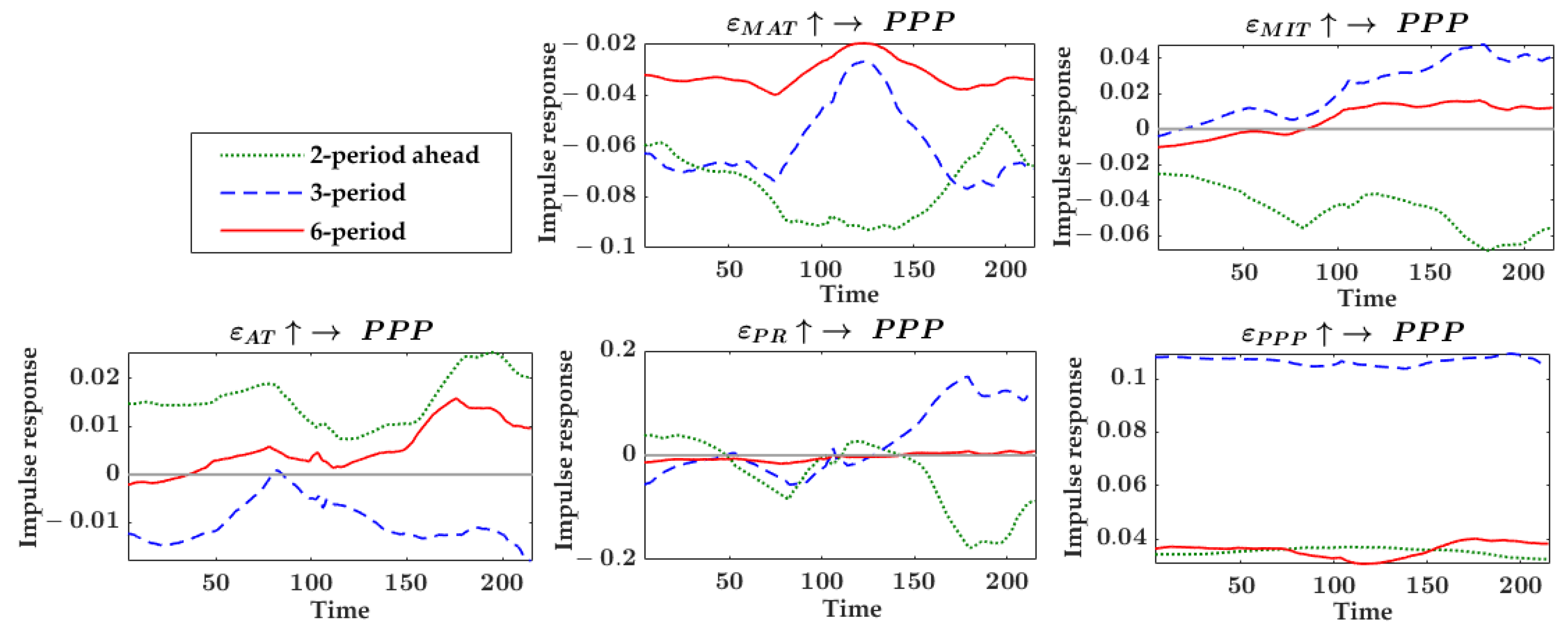
The VAR model could also generate a kind of impulse response results, but since the parameters of the model were not time-varying, the impulse response results only indicate the overall average so did not meet the analysis needs of this study. Nevertheless, the impulse response results still provide a useful reference value. Referring to the impulse response results generated by the VAR model of the pointed pepper analysis unit, the final selected intervals were lag 2 periods (also called 2-period ahead as shown in the equal-interval impulse response figures), lag 3 periods, and lag 6 periods, representing the short-, mid- and long-term, respectively. Figure 3. shows the equal-interval impulse response results of the pointed pepper analysis unit. For example, in Figure 3, “   ε M A T     P P P ” represents the positive shock of maximum temperature changes on pointed pepper price fluctuations by one-unit standard deviation, and the corresponding small graph is the equal-interval impulse response result of the price fluctuations to this shock. Therefore, the whole Figure 3 demonstrates the variations in the impacts of maximum temperature, minimum temperature, average temperature, precipitation, and the price of pointed pepper itself on the price of pointed pepper under different lag periods conditions.
As can be seen from Figure 3, the maximum temperature changes had negative impacts with significant time-varying characteristics on the price fluctuations of pointed pepper, and the short-term impact intensity was significantly stronger than the long-term. The short-term impact of minimum temperature on the price of pointed pepper was negative with the impact intensity tending to expand, while the mid-term and long-term impacts were mainly positive and also had a tendency to expand in intensity. The short- and long-term impacts of average temperature on pointed pepper prices were predominantly positive and time-varying, while the impacts with a lag of 3 periods (the mid-term impacts) were negative and also time-varying. The long-term impact intensity of precipitation on pointed pepper price was weak and near zero. The short-term and mid-term impacts of precipitation on pointed pepper price were time-varying in both direction and intensity with a relatively weaker intensity from the 1st to the 150th week. After about the 150th week, the mid-term impacts stayed positive and continued to expand until stabilizing at a higher intensity, while the short-term impacts stayed negative and continued to expand until stabilizing at a stronger intensity. Overall, the impact intensity of weather factors on pointed pepper was strongest in the short-term, and tended to zero value in the long-term. In recent years, the influence of precipitation and minimum temperature on pointed pepper prices had been tending to strengthen. In addition, we also explored the impacts of pointed pepper price fluctuations on itself, and the time-varying characteristic of the shocks was very weak, with the shocks’ intensity being strong in the lag 3rd period and weak in the lag 2nd and lag 6th periods.
  • Impulse Response Analysis at Different Time Points
For the impulse response analysis at different time points, it is necessary to select specific time points to analyze the life cycle of the impacts of weather changes on vegetable price fluctuations. According to the variance decomposition results, we generally selected the weather factor that had the strongest impact on the price fluctuations of the vegetable variety first. Then we checked the data fluctuations of that weather factor and selected the time points when the extreme value occurred. At last, we considered the historical weather disaster events information for the main producing area and the vegetable information such as the main production period and life cycle to select the final time points to be observed. The impulse response analysis at these time points could capture the response of vegetable price fluctuations to the occurrence of extreme weather.
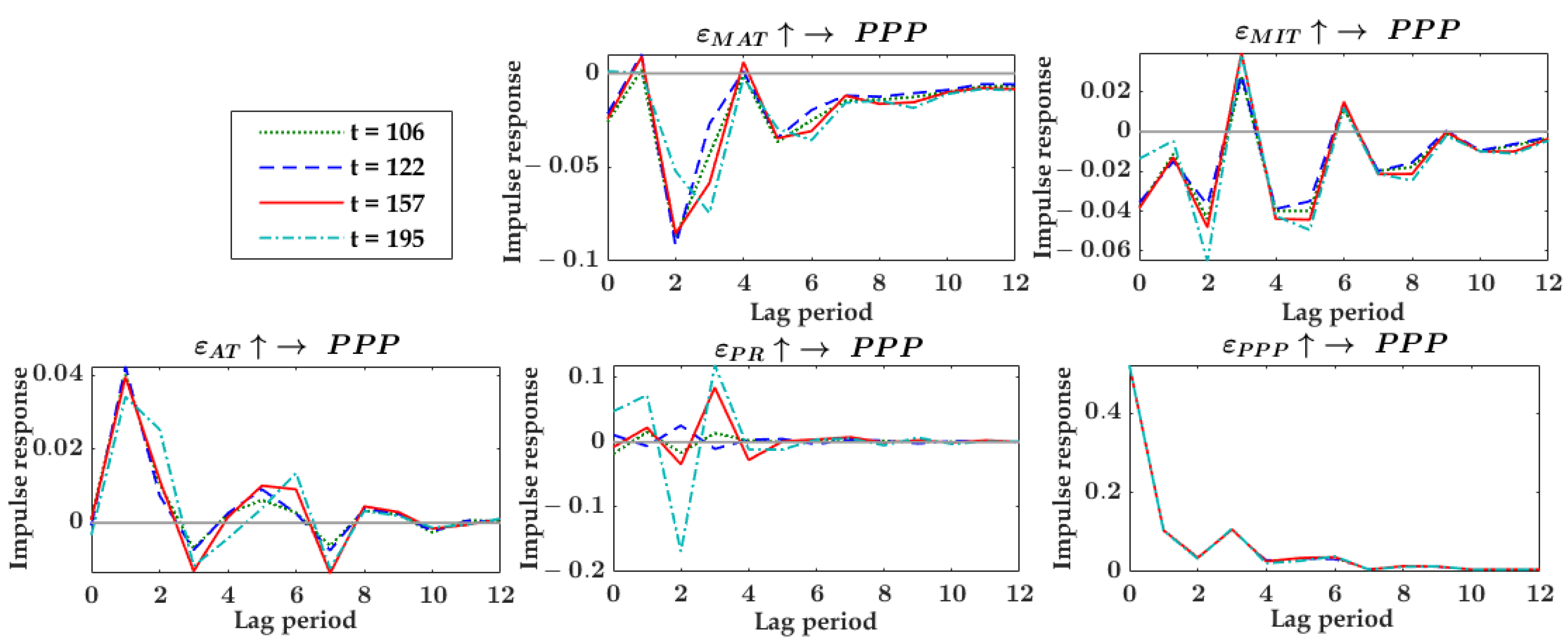
For pointed pepper analysis unit, the 106th, 122nd, 157th, and 195th weeks were selected as the analysis time points. The 106th week was 13–19 August 2018, which saw a positive precipitation fluctuation of 296.3 mm as Typhoon Rumbia passed through Shandong Province, causing widespread heavy rainfall and severe flooding in Weifang (Shouguang county belongs to Weifang), Shandong Province. The 122nd week was 3–9 December 2018, which saw negative fluctuations in maximum temperatures of 10.77 degrees Celsius and negative fluctuations in minimum temperatures of 7.73 degrees Celsius, with cold and windy weather in Shandong Province. The 157th week was 22–28 July 2019, and the positive fluctuation value of precipitation in that week was 244.2 mm. During that period, Shandong Province was in the rainy season, and the precipitation increased sharply and concentrated. The 195th week was from 27 April to 3 May 2020. The maximum temperature in that week increased sharply by 11.89 degrees Celsius, and the minimum temperature increased sharply by 7.42 degrees Celsius. The planting and harvesting of pointed peppers in Shandong Province can be done throughout spring, summer and autumn, and the time points selected for this study cover the planting and harvesting period and the selling off-season and peak season of pointed peppers.
Figure 4 shows the results of impulse response at different time points in pointed pepper analysis unit. There was a strong consistency in the dynamic impulse responses of pointed pepper price fluctuations to one-unit standard deviation positive change in weather factor occurring at the four different time points. The response of pointed pepper price fluctuations to maximum temperature changes occurring at the four time points was mainly negative, with the strongest response in the lag 2nd period and starting to converge to zero after the lag 5th period. The response of pointed pepper price fluctuations to the minimum temperature changes had a positive and negative alternating pattern, gradually converging to zero over time. The response of pointed pepper price fluctuations to the average temperature changes reached its strongest in the lag 1st period, and thereafter experienced positive and negative alternating variation until it was nearly zero in the lag 10th period. The response of pointed pepper price fluctuations to precipitation changes converged to zero in the lag 5th period. Compared to the other three time points chosen, the response of pointed pepper price fluctuations to the 195th week’s precipitation changes were the strongest and reached the strongest negative value in the lag 3rd period and the strongest positive value in the lag 4th period. The intensity of the impulse response of the pointed pepper price fluctuations to precipitation changes increased throughout the time domain (from the 106th week to the 195th week), while the response mechanism to temperature varied weakly. In terms of the life cycle length of the dynamic impacts, the impulse response of pointed pepper prices to precipitation lasted about 5 lag periods, while the impulse response to temperature lasted at least 10 lag periods to disappear. In terms of the intensity of the impacts, the strongest impact of temperature and precipitation on the pointed pepper price mainly occurred within 2 lag periods, and the strongest impact of precipitation on pointed pepper price exceeded the temperature’s strongest impact. In addition, the impacts of the pointed pepper price fluctuations occurring at the four time points on itself were highly consistent and positive with the impact intensity gradually weakening, and almost disappearing after the lag 10th period. Since the equal-interval impulse responses of pointed pepper price fluctuations to itself were weakly time-varying, the life cycle of the time point impulse response was stable. These findings above have guiding significance for relevant economic activities.

4.3.2. Loofah, Chinese Chives and Tomato Analysis Units

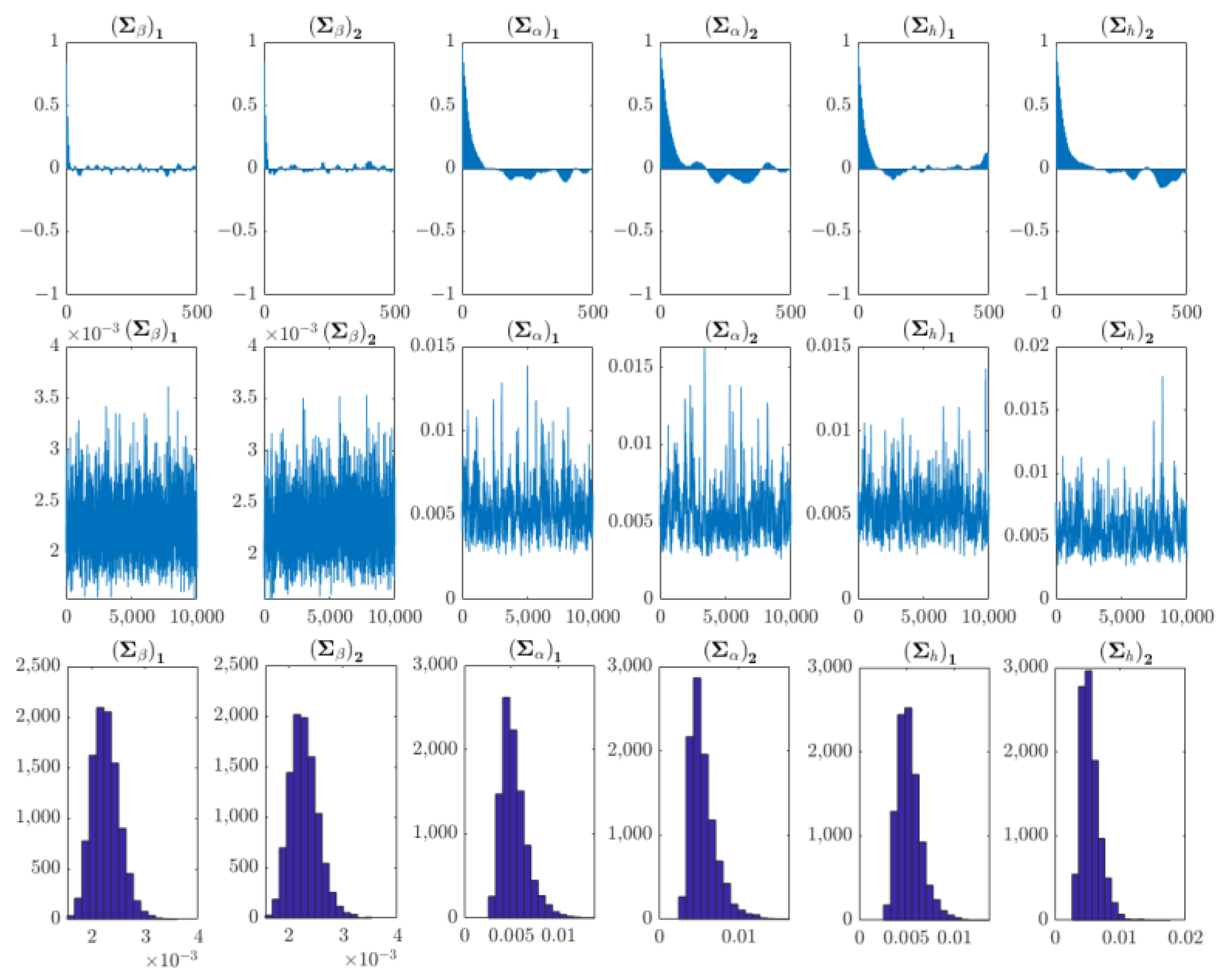
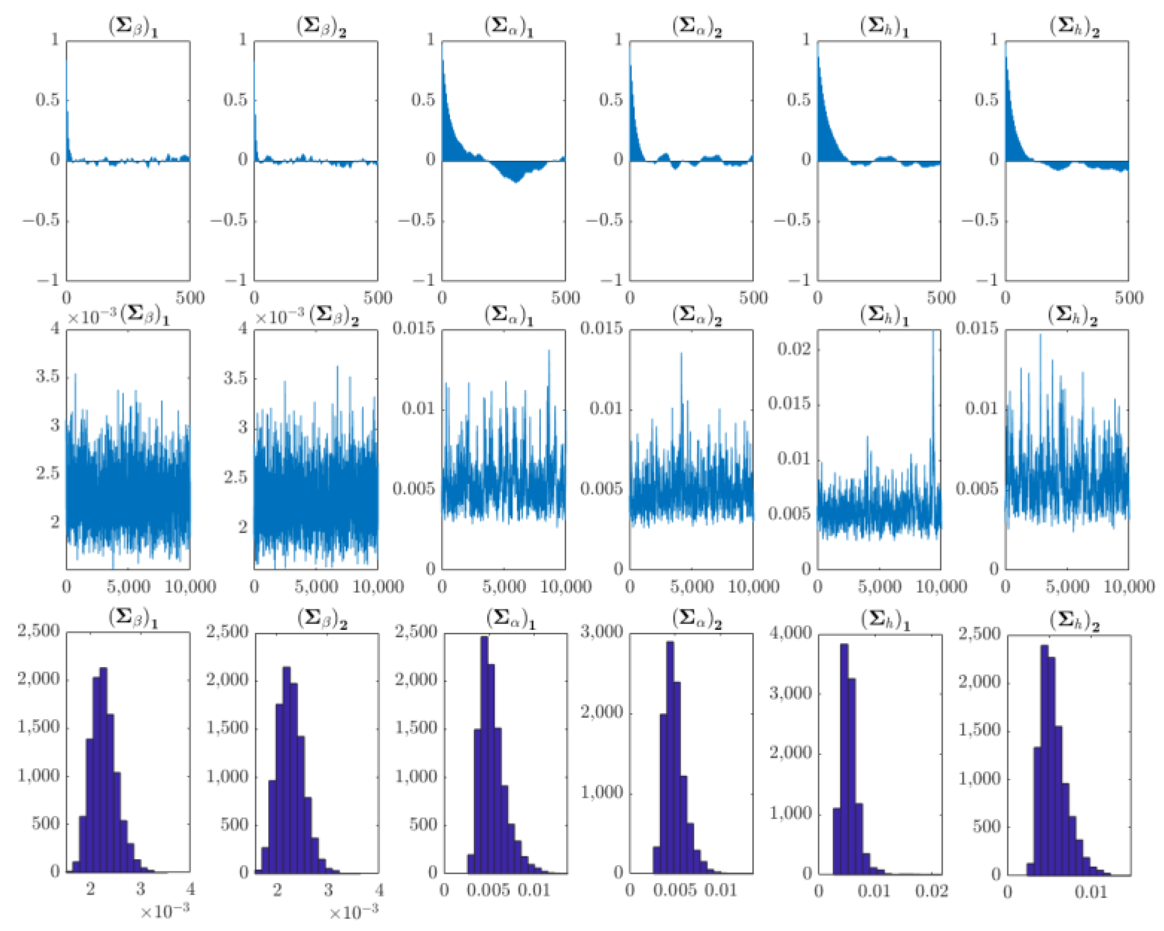
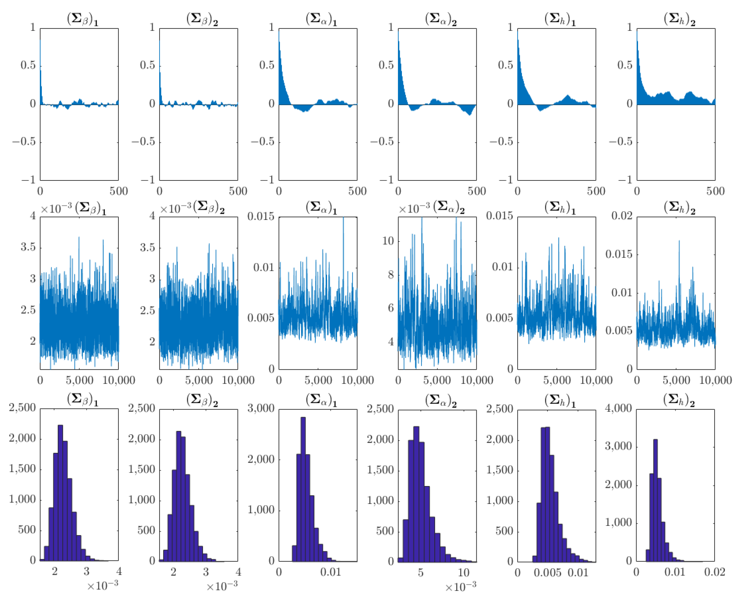
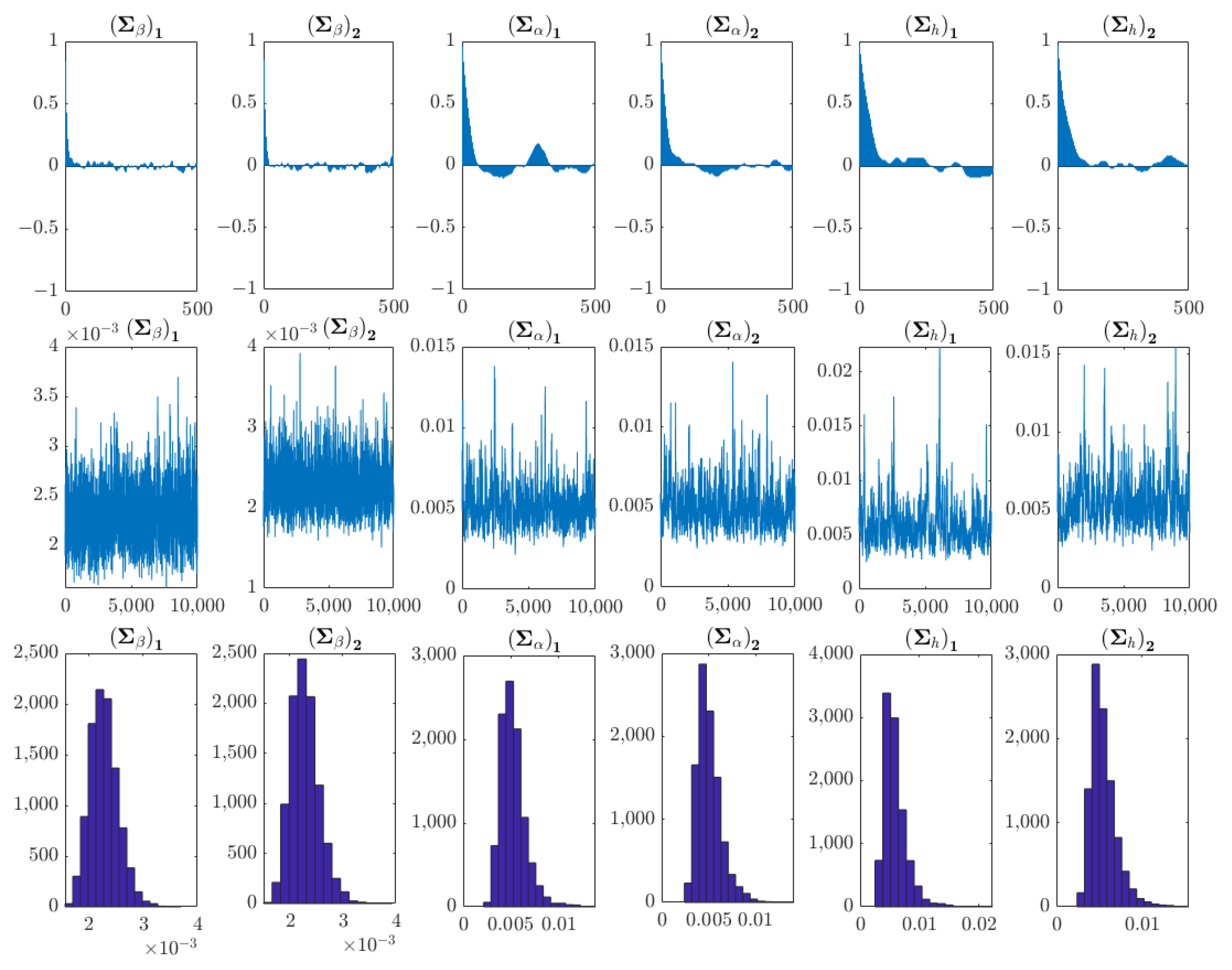
There were four analysis units in this study: pointed pepper, loofah, Chinese chives and tomato. The TVP-VAR model and impulse response analysis was performed for the loofah, Chinese chives and tomato analysis units following the analysis procedure of the pointed pepper analysis unit. The model estimation and parameter test results for loofah, Chinese chives, and tomato analysis units are shown in Table A2, Table A3 and Table A4 in Appendix A and Figure A1, Figure A2 and Figure A3 in Appendix B. In the same way as the judgment of the pointed pepper analysis unit, the related results indicated that the TVP-VAR models constructed in this study for the loofah, Chinese chives, and tomato analysis units could be used for subsequent impulse response analysis. The intervals and specific time points used for impulse response analysis for each analysis unit were selected in the same way as for the pointed pepper analysis unit.
Table 9 summarizes the TVP-VAR model information for the four analysis units. (1) The variables in the loofah TVP-VAR model were maximum and average temperature, minimum relative humidity, sunshine duration, and loofah price. The optimal lag order of the model was set to 5. The final selected intervals for impulse response analysis were lag 2 periods, lag 4 periods, and lag 6 periods, and the selected specific time points were the 86th, 122nd, 159th, and 195th weeks. (2) The variables in the Chinese chives TVP-VAR model were maximum and average temperature, and Chinese chives price. The optimal lag order of the model was set to 4. The final selected intervals for impulse response analysis were lag 2 periods, lag 3 periods, and lag 6 periods, and the selected specific time points were the 28th, 86th,122nd, and 195th weeks. (3) The variables in the tomato TVP-VAR model were maximum and average temperature, sunshine duration, and tomato price. The optimal lag order of the model was set to 8. The final selected intervals for impulse response analysis were lag 1 period, lag 3 periods, and lag 6 periods, and the selected specific time points were the 86th, 122nd, 159th, and 195th weeks.
  • Loofah
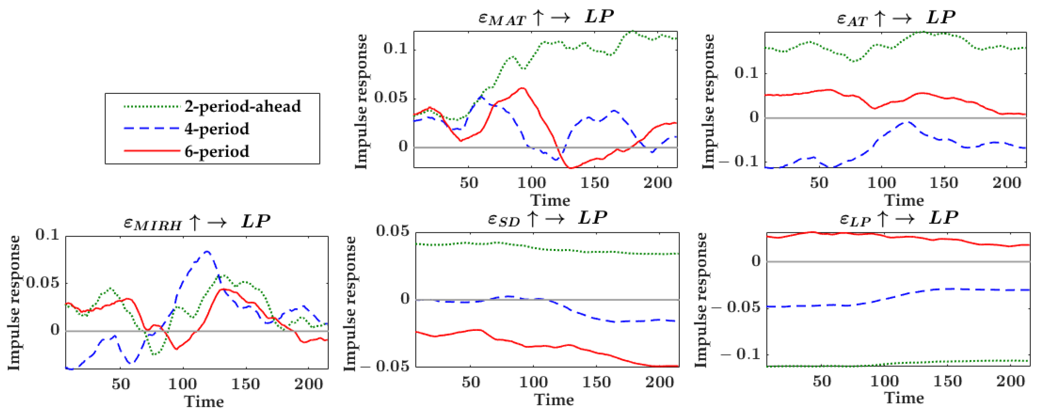
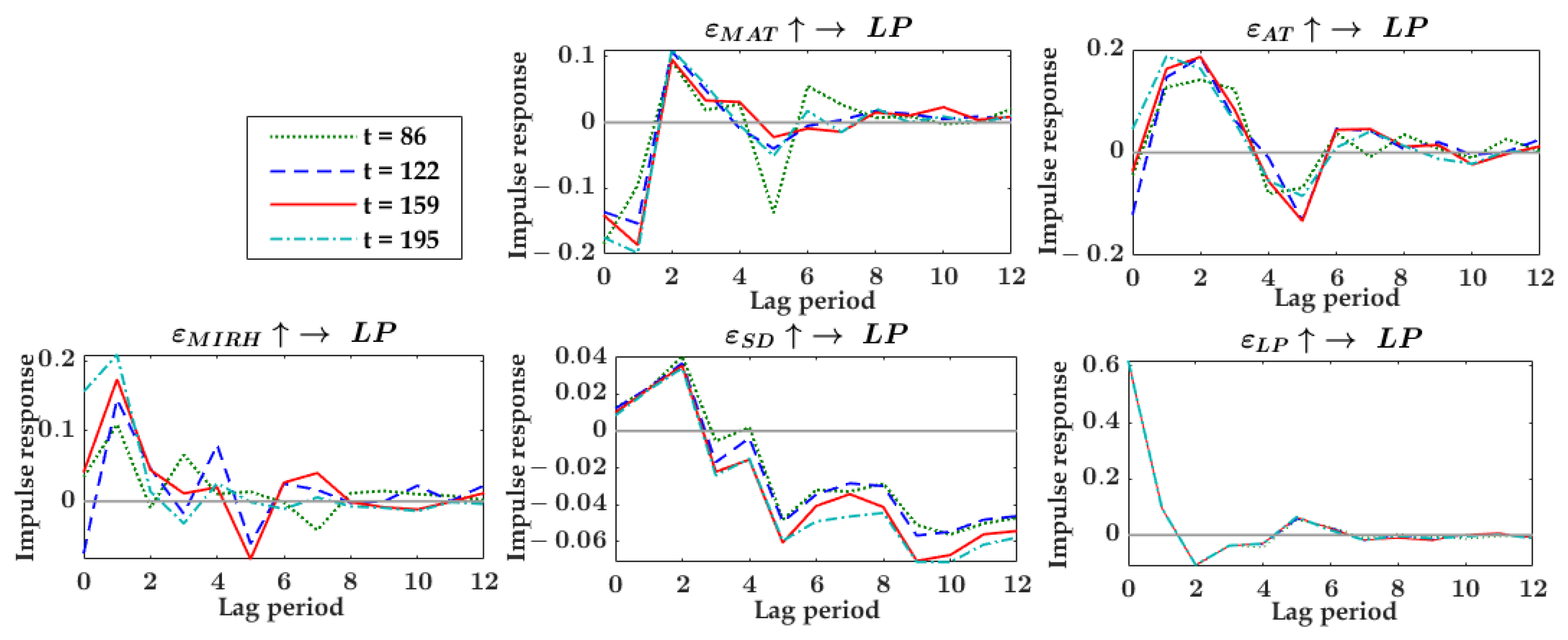
The results of the equal-interval impulse response and the time point impulse response of the loofah analysis unit are shown in Figure A4 and Figure A5 in Appendix B. As you can see, these figures clearly show all the impulse response results that belong to the loofah analysis unit. The interpretation method of the figure meaning is the same as that of the pepper analysis unit. Therefore, the impulse response results of the loofah analysis unit (as well as the Chinese chives and tomato analysis units) no longer were described in detail here, only the main and outstanding features were described. For equal-interval impulse response results, the dynamic impacts of maximum temperature and minimum relative humidity changes on loofah price fluctuations were strongly time-varying. While the time-varying characteristics of the impacts of average temperature and sunshine duration changes on loofah price fluctuations were weak, and the trend of shocks variation was relatively smooth. The equal-interval impacts of loofah price fluctuations on itself varied smoothly more.
For time point impulse response results, there was relatively strong consistency in the dynamic impacts of weather changes occurring at the four time points selected on loofah price fluctuations. In terms of the life cycle length of the dynamic impacts, the impulse response of loofah price to temperature and relative humidity lasted about 11 lag periods, while the impulse response to sunshine duration exceeded 27 lag periods. In terms of impact intensity, the strongest impacts of temperature and relative humidity on the loofah price mainly occurred within 2 lag periods and were stronger than that of sunshine duration, and the strongest impact of sunshine duration on loofah price happened in the lag 9th period. In addition, the dynamic impacts of loofah price fluctuations occurring at the four selected time points on itself were nearly the same.
2.
Chinese Chives
The results of the equal-interval impulse responses and the time point impulse responses of the Chinese chives analysis unit are shown in Figure A6 and Figure A7 in Appendix B. For equal-interval impulse response results, the time-varying characteristics of the impacts of maximum temperature changes on price fluctuations were more obvious than that of average temperature. The impacts of Chinese chives price fluctuations on itself were also weakly time-varying.
For time point impulse response results, the impacts of specific weather factor changes occurring at the four selected time points on Chinese chives price fluctuations were also highly consistent. In terms of the life cycle length of the dynamic impacts, the impulse response of Chinese chives prices to temperature lasted about 12 lag periods. In terms of the intensity of the impacts, the strongest impact of temperature on the Chinese chives price occurred in the lag 1st period. The life cycle and intensity variation of the dynamic impacts of Chinese chives price fluctuations occurring at the four selected time points on itself were almost the same.
3.
Tomato
The results of the equal-interval impulse responses and the time point impulse responses of the tomato analysis unit are shown in Figure A8 and Figure A9 in Appendix B. For equal-interval impulse response results, the dynamic impacts of maximum temperature, average temperature and sunshine duration changes on price fluctuations had certain time-varying characteristics. The equal-interval impacts of tomato price fluctuations on itself were relatively smooth as same as other three vegetables in this study.
The time point impulse response results of the tomato analysis unit show once again, the weather changes occurring at the four time points had a relatively strong consistency in influencing price fluctuations. The impact of maximum temperature and average temperature on tomato price had a positive and negative alternating trend. The shocks of sunshine duration on tomato price remained highly consistent from the current period to the lag 4th period. After the lag 5th period, the shock intensity showed an expanding trend from the 86th week to the 185th week. In terms of the life cycle length of the dynamic impacts, the impulse response of tomato prices to temperature lasted about 16 lag periods, while the impulse response to sunshine duration lasted for more than 27 lag periods. In addition, the life cycle and intensity variation of the dynamic impacts of tomato price fluctuations occurring at the four selected time points on itself were highly consistent as same as other three vegetables in this study.
For the same set of independent and dependent variables, if the impulse response results of each kind of equal-intervals and all time points were generated, the global impulse response results of a 3D curved surface would be obtained. Based on such a global awareness, the above analysis of equal-interval and time point impulse responses would be more accurately understood and grasped. The time point impulse response of vegetable price fluctuations to weather changes had a certain life cycle, which means that vegetable price fluctuations would not only be impacted by the current weather changes, but also be affected by several lag periods of the weather changes, and the impacts varied in different lag periods. The life cycle length and shocks trends of the time point impulse response would be different due to different independent and dependent variables, but the life cycle characteristics of the time point impulse response between the same independent variable and dependent variable were relatively stable. The equal-interval impulse response was actually the impulse response of vegetable price fluctuations to weather changes in the same lag period. The equal-interval impulse response of vegetable price fluctuations to weather changes was time-varying, and the time-varying characteristics (direction, amplitude and frequency) would vary with different intervals, as well as with different independent and dependent variables.
Based on the above analysis, it could generalizes as following: (1) The equal-interval impulse responses of vegetable price fluctuations to changes in temperature, precipitation and relative humidity had relatively stronger time-varying characteristics, and had relatively weaker time-varying characteristics to changes in sunshine duration. (2) The time point impulse response of vegetable price to temperature and relative humidity generally lasted about 12 lag periods, as for precipitation, which generally lasted 5 lag periods. Their overall shocks would gradually dissipate in a pattern of positive and negative alternating, with the strongest positive and negative intensity both occurring within 5 lag periods. As for sunshine duration, the time point impulse response would generally exceed 27 lag periods, with the strongest positive and negative intensity both occurring within 9 lag periods. Its shocks would generally be negative after the lag 5th period, which would last for a long time. (3) The time-varying characteristics for the equal-interval impulse response of vegetable price fluctuations to its own was very weak. The time point impulse response of vegetable price fluctuations to itself generally lasted for 10 lag periods, and the overall shocks intensity would gradually dissipate in a trend of fluctuations during the entire impulse response life cycle. The shocks were always positive in the current period and the lag 1st period. In addition, the lag 5th period is a notable time point in the time point impulse response of vegetable price fluctuations to itself.

4.4. Discussion

The price of commodity is determined by value and influenced by supply and demand. Weather factors, as exogenous shocks, can affect the market prices of agricultural products through the supply-demand balance mechanism by mainly influencing the quantity and quality of agricultural products supply. The possible impact paths of weather changes on vegetable prices are as follows: (1) Weather changes may affect the growth process of vegetables, prolong or shorten the growth cycle of vegetables, cause the vegetable harvest time to deviate from the normal time or the expected time, interfere with the market, and impact the market prices. (2) weather changes may cause fluctuations in vegetable production, and unstable supply may cause market price fluctuations. In particular, the occurrence of extreme weather may lead to a reduction in vegetable production, a shortage of supply in the market, and an abnormal rise in prices [33]. (3) Vegetables are fresh agricultural products, and due to their physiological response characteristics, their quality may be affected by weather factors to varying degrees in the process of growth, transportation and sales, thereby affecting their market prices [19,31]. (4) The occurrence of weather disasters may not only affect vegetable production activities, but also affect vegetable transportation and vegetable market trading activities, increasing the transaction costs of vegetables and eventually impacting market prices. (5) Product prices may be affected by the economic behavior of market participants. Vegetable market participants involve farmers, wholesalers, retailers and consumers, etc. Weather changes and weather disasters may affect the expectations (especially the price anticipation) and trading decisions and behavior (such as whether to trade and trade timing and volume) of these participants, which may affect the stability of market supply and demand in a short term, and finally lead to the price fluctuations [27]. (6) The release of information related to the impacts of weather changes on vegetable economy (including the loss of vegetable production caused by agrometeorological disasters, the interruption of vegetable transportation, the abnormal price fluctuations and the price forecast and early warning, etc.), the resulting online public opinion and the government’s response policies (mainly involving measures to deal with agrometeorological disasters, maintain vegetable supply and stabilize vegetable prices) may also be feasible paths for weather changes to impact vegetable prices. With impact paths such as these, and with weather changes as the independent variable and vegetable price as the ultimate dependent variable, the two can always be reasonably related through some paths and mechanism of influence. In fact, the paths of the dynamic impacts of weather changes on vegetable price fluctuations actually constitutes a complex dynamic path network, which makes the impacts go through a complex dynamic transmission process.
Weather factors are very normative time series data, which are highly deterministic, it is a relatively economical and practical approach to using weather factors as important observed variables when exploring the factors influencing vegetable price fluctuations. No matter how complicated the transmission process of the impacts of weather changes on vegetable price is, it will eventually get feedback on the fluctuations of vegetable prices. This study empirically found that by directly examining the impact and response mechanism between changes in weather factors and vegetable price fluctuations, some stable conclusions and patterns were really drawn. It is feasible to treat the complex dynamic impact path network as a black box, but this is only a temporary treatment. We will systematically explore the internal mechanism of this dynamic impact in the next step. We speculate that in the complex dynamic network of impact transmission, when the shock of weather changes (as an exogenous variable) is closer to the price target, its shock effect is also more likely to be affected by shocks from more other complex variables. Therefore, we speculate that the dynamic impact mechanism of weather changes on vegetable price fluctuations may be altered to some extent or even no longer so stable due to significant changes in the moderating role of other key variables. Of course, this speculation will not deny the reliability of the results and conclusions of this study, but will help to better interpret the results. An important condition for this study to obtain stable and reliable rules may be that the moderating effect of other key variables under the specific spatial-temporal conditions of this study has not changed significantly, and it is not enough to destroy the core impact mechanism of weather changes on vegetable price fluctuations. In addition, another very important reason is that the model we built allows the change of external conditions and can capture the dynamic change of impacts. Our purpose was to prove and analyze the dynamic impacts of weather changes on vegetable price fluctuations. We believe that the primary task to explore the internal mechanism of dynamic impacts is to identify key moderating variables and analyze their moderating mechanism, which will undoubtedly expand and deepen our research topic, help optimize the existing model and clearly explain the reasons for the results of this study.
Based on the above analysis, it should be emphasized again that the results of this study are under specific spatial-temporal conditions, and the generalization of the conclusion needs to be further verified. The general and specific conclusions of this study should be distinguished. Of course, we hope that the model constructed and the research results obtained in this study can guide the practice, but its practical value and guiding effect need to be further tested. Theoretically, on the basis of sufficient and high-quality relevant data, the research method in this study can be used to analyze the dynamic impact of weather changes on vegetable price fluctuations under any spatial-temporal conditions, and the dynamic impacts can be continuously followed up and updated. In addition, the methods in this study can be used to further empirically explore other possible influencing factors of vegetable price fluctuations. Weather change is only one of the important factors affecting vegetable prices. How it functions together with other key factors needs more research. These explorations can not only enrich the research results of vegetable price fluctuations, but also contribute to the research of vegetable price prediction and early warning, etc. The research findings can also provide decision-making and behavior basis for market participants and policy makers, so as to help ensure the stable supply and price of vegetables and the healthy and prosperous development of vegetable industry.

5. Conclusions and Suggestions

5.1. Conclusions

In this study, the Granger causality test was utilized to demonstrate the Granger causality between changes in weather factors and vegetable price fluctuations by taking weather factors and vegetable prices in the main producing areas as the research objects. VAR models were constructed for variance decomposition analysis, and TVP-VAR models were constructed for equal-interval and time point impulse responses. Specific results on the dynamic impacts of particular weather factors on price fluctuations of pointed pepper, loofah, Chinese chives and tomato were derived and further generalizations of the research findings were made. The main conclusions were these: (1) Weather changes in the main producing areas did have impacts on vegetable price fluctuations. (2) Price fluctuations of specific vegetable species were subject to shocks from changes in specific weather factors, and the contribution weight of each weather factor to the impacts on vegetable price fluctuations could be derived through variance decomposition. (3) The equal-interval impulse response of vegetable price fluctuations to changes in weather factors was time-varying to some extent, and the intensity and direction of the impacts of changes in weather factors in specific lag periods on vegetable price fluctuations also varied in different degrees. (4) The trends of variation in the impacts of one-unit standard deviation positive change in particular weather factors occurring at each abnormal weather time point on the fluctuations of particular vegetable price were highly consistent, so the effect of the impacts of abnormal change in particular weather factors on the fluctuations of vegetable price was graspable. (5) Vegetable price fluctuations was most affected by its own lag period. The equal-interval shock effects of vegetable price fluctuations on itself were highly stable. The impacts of vegetable price fluctuations of one- unit standard deviation occurring at different time points on the vegetable price itself were highly consistent, and the characteristics of the changes in the impacts were smoothly moving from positive strong shocks to final dissipation.

5.2. Suggestions

(1) We can attempt to weaken the impacts of weather disasters on vegetable economy from various aspects, and ultimately reduce its impacts on vegetable price fluctuations. For example, based on the methods and findings of this research, relatively sensitive vegetable varieties and important weather factors can be screened out from the perspectives of vegetable varieties and weather factors, so as to help develop targeted and finely differentiated agricultural insurance varieties. The practical experience proves that relevant government policies have played an indispensable role in coping with agricultural meteorological disasters and ensuring supply and price stability of vegetables. In addition, presumably, we may from the entire supply chain process of vegetable cultivation to sale to try to weaken the impacts of weather disaster on vegetable price, such as promoting greenhouses planting, developing urban vertical agriculture, enhancing the preservation storage and transport capacity, shortening the supply chain, improving agricultural meteorological disaster and vegetables price fluctuation early warning capability and efficiency of information release, etc. However, the actual effects of these measures still need to be tested in practice, and the laws and logic contained in them still need to be scientifically proved in a lot of studies.
(2) The research on the dynamic impact mechanism of weather factors on vegetable prices should be further expanded, and the internal mechanism should be systematically and deeply explored. On the one hand, we should focus on summarizing general and regular knowledge, on the other hand, we should form specialized knowledge under a specific time and space to guide specific practice, and insist on combining the generality of theoretical knowledge with the particularity of specific practical application. These research results help to determine the role of climate and weather changes in agricultural economy development, and provide theoretical and practical references for timely adjustment of agricultural economic activities and further optimization of adaptive policy systems.

Author Contributions

Conceptualization, H.Y.; methodology, H.Y.; software, H.Y., Y.C. and Y.W.; validation, Y.C., Y.S. and Y.W.; formal analysis, H.Y., Y.C., Y.W. and W.G.; investigation, Y.S., Y.W., W.G. and H.F.; resources, Y.L., H.Y. and H.F.; data curation, Y.L., Y.C. and Y.S.; writing—original draft preparation, H.Y.; writing—review and editing, H.Y.; visualization, Y.C., Y.S. and Y.W.; supervision, H.Y. and Y.L.; project administration, H.Y. and funding acquisition, Y.L. All authors have read and agreed to the published version of the manuscript.

Funding

This research was funded by the National Social Science Foundation of China (Project No. 21BGL168).

Data Availability Statement

Not applicable.

Conflicts of Interest

The authors declare no conflict of interest.

Appendix A

Table A1. Stationary test.
First-Level VariablesSecondary VariablesCodeADFPPConclusions
InterceptTrend and InterceptNoneInterceptTrend and InterceptNone
Vegetable
prices
D pointed pepper pricePPP−6.125867 ***−6.110883 ***−6.130357 ***−14.37946 ***−14.35091 ***−14.39663 ***Stationary
D loofah priceLP−11.48933 ***−11.47608 ***−11.51571 ***−11.62354 ***−11.59984 ***−11.65401 ***Stationary
D Chinese chives priceCCP−10.19264 ***−10.16857 ***−10.21698 ***−10.22133 ***−10.19745 ***−10.24536 ***Stationary
D tomato priceTP−10.25838 ***−10.25092 ***−10.27605 ***−10.25838 ***−10.25092 ***−10.27605 ***Stationary
Weather
factors
in Shouguang
D maximum temperatureMAT−20.0715 ***−20.08556 ***−20.11769 ***−19.10048 ***−19.10710 ***−19.13434 ***Stationary
D minimum temperatureMIT−5.24486 ***−5.230246 ***−5.256803 ***−17.48307 ***−17.49313 ***−17.50212 ***Stationary
D average temperatureAT−4.713818 ***−4.709089 ***−4.724847 ***−18.54082 ***−18.53967 ***−18.5653 ***Stationary
D precipitationPR−14.19014 ***−14.15539 ***−14.22388 ***−50.26337 ***−50.37139 ***−50.53741 ***Stationary
D maximum relative humidityMARH−11.97051 ***−11.9637 ***−11.99922 ***−28.52883 ***−28.92497 ***−28.61517 ***Stationary
D minimum relative humidityMIRH−15.11913 ***−15.10502 ***−15.15052 ***−26.97608 ***−26.97608 ***−27.44539 ***Stationary
D sunshine durationSD−5.946357 ***−5.900428 ***−5.961565 ***−7.311444 ***−7.312367 ***−7.314433 ***Stationary
Weather
factors
in Changle
D maximum temperatureMAT−20.71488 ***−20.72627 ***−20.7626 ***−19.53424 ***−19.54433 ***−19.56966 ***Stationary
D minimum temperatureMIT−5.41871 ***−5.396147 ***−5.430856 ***−18.45126 ***−18.45187 ***−18.47337 ***Stationary
D average temperatureAT−4.601533 ***−4.590126 ***−4.612283 ***−19.29557 ***−19.29395 ***−19.32213 ***Stationary
D precipitationPR−11.83259 ***−11.80236 ***−11.86127 ***−78.47304 ***−78.18714 ***−78.80674 ***Stationary
D maximum relative humidityMARH−12.1011 ***−12.10656 ***−12.13014 ***−24.22536 ***−24.37019 ***−24.29398 ***Stationary
D minimum relative humidityMIRH−14.43345 ***−14.42353 ***−14.46221 ***−24.34848 ***−24.40541 ***−24.42056 ***Stationary
D sunshine durationSD−7.168282 ***−7.125036 ***−7.186744 ***−5.259499 ***−5.24769 ***−5.263488 ***Stationary
*** indicate the statistical significance at the 1% levels, respectively.
Table A2. TVP-VAR model estimation results of the loofah analysis unit.
ParameterMeanStd. Dev.95% L95% UG. C. D.I. F.
β 1 0.00230.00030.00180.00280.9898.71
β 2 0.00230.00030.00180.00290.1668.59
α 1 0.00530.00140.00330.00890.39242.96
α 2 0.00550.00170.00340.01000.94757.63
h 1 0.00530.00130.00340.00840.12836.21
h 2 0.00550.00150.00340.00900.79551.96
Note: TVP-VAR model (Lag = 5) Iteration: 10,000 Sigma ( β ): Diagonal.
Table A3. TVP-VAR model estimation results of the Chinese chives analysis unit.
ParameterMeanStd. Dev.95% L95% UG. C. D.I. F.
β 1 0.00230.00030.00180.00290.16710.48
β 2 0.00230.00030.00180.00280.36711.7
α 1 0.00540.00150.00340.00910.28361.77
α 2 0.00490.00120.00330.00780.04138.74
h 1 0.00550.00160.00330.00920.28469.18
h 2 0.00560.00160.00340.00950.61352.94
Note: TVP-VAR model (Lag = 4) Iteration: 10,000 Sigma ( β ): Diagonal.
Table A4. TVP-VAR model estimation results of the tomato analysis unit.
ParameterMeanStd. Dev.95% L95% U G. C. D.I. F.
β 1 0.00230.00030.00180.00290.5099.46
β 2 0.00230.00030.00180.00290.12411.84
α 1 0.00530.00140.00340.00870.02839.97
α 2 0.00500.00130.00330.00810.43739.57
h 1 0.00540.00150.00340.00930.00056.85
h 2 0.00540.00150.00340.00900.38378.87
Note: TVP-VAR model (Lag = 8) Iteration: 10,000 Sigma ( β ): Diagonal.

Appendix B

Figure A1. Sample autocorrelation, sample path and posterior density diagrams of the loofah analysis unit.
Agronomy 12 02680 g0a1
Figure A2. Sample autocorrelation, sample path and posterior density diagrams of the Chinese chives analysis unit.
Agronomy 12 02680 g0a2
Figure A3. Sample autocorrelation, sample path and posterior density diagrams of the tomato analysis unit.
Agronomy 12 02680 g0a3
Figure A4. Equal-interval impulse response in the loofah analysis unit. ε   = positive shocks of one-unit standard deviation; LP = D loofah price; MAT = D maximum temperature; AT = D average temperature; MIRH = D minimum relative humidity; SD = D sunshine duration.
Agronomy 12 02680 g0a4
Figure A5. Impulse response at different time points in the loofah analysis unit. ε   = positive shocks of one-unit standard deviation; LP = D loofah price; MAT = D maximum temperature; AT = D average temperature; MIRH = D minimum relative humidity; SD = D sunshine duration.
Agronomy 12 02680 g0a5
Figure A6. Equal-interval impulse response in the Chinese chives analysis unit. ε   = positive shocks of one-unit standard deviation; CCP = D Chinese chives price; MAT = D maximum temperature; AT = D average temperature.
Agronomy 12 02680 g0a6
Figure A7. Impulse response at different time points in the Chinese chives analysis unit. ε   = positive shocks of one-unit standard deviation; CCP = D Chinese chives price; MAT = D maximum temperature; AT = D average temperature.
Agronomy 12 02680 g0a7
Figure A8. Equal-interval impulse response in the tomato analysis unit. ε   = positive shocks of one-unit standard deviation; TP = D tomato price; MAT = D maximum temperature; AT = D average temperature; SD = D sunshine duration.
Agronomy 12 02680 g0a8
Figure A9. Impulse response at different time points in the tomato analysis unit. ε   = positive shocks of one-unit standard deviation; TP = D tomato price; MAT = D maximum temperature; AT = D average temperature; SD = D sunshine duration.
Agronomy 12 02680 g0a9

References

  1. Li, Y.; Zhang, M.; Liu, J.; Su, B.; Lin, X.; Liang, Y.; Bao, Y.; Yang, S.; Zhang, J. Research on the Disturbance Sources of Vegetable Price Fluctuation Based on Grounded Theory and LDA Topic Model. Agriculture 2022, 12, 648. [Google Scholar] [CrossRef]
  2. Li, Y.; Xia, J.; Li, C.; Zheng, M. Construction of an Early-Warning System for Vegetable Prices Based on Index Contribution Analysis. Sustainability 2015, 7, 3823–3837. [Google Scholar] [CrossRef] [Green Version]
  3. Illankoon, I.; Kumara, B. Analyzing the Influence of Various Factors for Vegetable Price using Data Mining. In Proceedings of the International Research Conference 2020 KDU, Ratmalana, Sri Lanka, 15–16 October 2020. [Google Scholar]
  4. Li, Y.; Liu, J.; Yang, H.; Chen, J.; Xiong, J. A Bibliometric Analysis of Literature on Vegetable Prices at Domestic and International Markets—A Knowledge Graph Approach. Agriculture 2021, 11, 951. [Google Scholar] [CrossRef]
  5. Ji, L.; Li, C.; Zhang, S. The spatial distribution of vegetable production in China and its impact on vegetable price volatility. Econ. Geogr. 2016, 36, 148–155. [Google Scholar]
  6. Adams, R.M.; Hurd, B.H.; Lenhart, S.; Leary, N. Effects of global climate change on agriculture: An interpretative review. Clim. Res. 1998, 11, 19–30. [Google Scholar] [CrossRef] [Green Version]
  7. Hatfield, J.L.; Boote, K.J.; Kimball, B.A.; Ziska, L.H.; Izaurralde, R.C.; Ort, D.; Thomson, A.M.; Wolfe, D. Climate impacts on agriculture: Implications for crop production. Agron. J. 2011, 103, 351–370. [Google Scholar] [CrossRef] [Green Version]
  8. Gordeev, R.V.; Pyzhev, A.I.; Zander, E.V. Does Climate Change Influence Russian Agriculture? Evidence from Panel Data Analysis. Sustainability 2022, 14, 718. [Google Scholar]
  9. Vermeulen, S.J.; Aggarwal, P.K.; Ainslie, A.; Angelone, C.; Campbell, B.M.; Challinor, A.J.; Hansen, J.W.; Ingram, J.S.; Jarvis, A.; Kristjanson, P. Options for support to agriculture and food security under climate change. Environ. Sci. Policy 2012, 15, 136–144. [Google Scholar] [CrossRef]
  10. Eigenbrod, C.; Gruda, N. Urban vegetable for food security in cities. A review. Agron. Sustain. Dev. 2015, 35, 483–498. [Google Scholar] [CrossRef] [Green Version]
  11. Tack, J.B.; Holt, M.T. Influence of weather extremes on the spatial correlation of corn yields. Clim. Chang. 2016, 134, 299–309. [Google Scholar] [CrossRef]
  12. Lesk, C.; Rowhani, P.; Ramankutty, N. Influence of extreme weather disasters on global crop production. Nature 2016, 529, 84–87. [Google Scholar] [CrossRef] [PubMed] [Green Version]
  13. Jat, M.L.; Dagar, J.C.; Sapkota, T.B.; Govaerts, B.; Ridaura, S.L.; Saharawat, Y.S.; Sharma, R.K.; Tetarwal, J.P.; Jat, R.K.; Hobbs, H. Climate change and agriculture: Adaptation strategies and mitigation opportunities for food security in South Asia and Latin America. Adv. Agron. 2016, 137, 127–235. [Google Scholar]
  14. De Winne, J.; Peersman, G. The adverse consequences of global harvest and weather disruptions on economic activity. Nat. Clim. Chang. 2021, 11, 665–672. [Google Scholar] [CrossRef]
  15. Furuya, J.; Kobayashi, S. Impact of global warming on agricultural product markets: Stochastic world food model analysis. Sustain. Sci. 2009, 4, 71–79. [Google Scholar] [CrossRef]
  16. Wang, J.; Mendelsohn, R.; Dinar, A.; Huang, J.; Rozelle, S.; Zhang, L. The impact of climate change on China’s agriculture. Agric. Econ. 2009, 40, 323–337. [Google Scholar] [CrossRef]
  17. Seo, S.N. An essay on the impact of climate change on US agriculture: Weather fluctuations, climatic shifts, and adaptation strategies. Clim. Chang. 2013, 121, 115–124. [Google Scholar] [CrossRef]
  18. Cogato, A.; Meggio, F.; De Antoni Migliorati, M.; Marinello, F. Extreme weather events in agriculture: A systematic review. Sustainability 2019, 11, 2547. [Google Scholar] [CrossRef] [Green Version]
  19. Dalhaus, T.; Schlenker, W.; Blanke, M.M.; Bravin, E.; Finger, R. The effects of extreme weather on apple quality. Sci. Rep. 2020, 10, 1–7. [Google Scholar] [CrossRef]
  20. Cui, Q.; Ali, T.; Xie, W.; Huang, J.; Wang, J. The uncertainty of climate change impacts on China’s agricultural economy based on an integrated assessment approach. Mitig. Adapt. Strat. Glob. 2022, 27, 1–22. [Google Scholar] [CrossRef]
  21. Poudel, M.P.; Chen, S.E.; Huang, W.C. Pricing of rainfall index insurance for rice and wheat in Nepal. J. Agric. Sci. Technol. 2016, 18, 291–302. [Google Scholar]
  22. Elum, Z.A.; Nhamo, G.; Antwi, M.A. Effects of climate variability and insurance adoption on crop production in select provinces of South Africa. J. Water Clim. Change 2018, 9, 500–511. [Google Scholar] [CrossRef]
  23. Guo, J.; Jin, J.; Tang, Y.; Wu, X. Design of Temperature Insurance Index and Risk Zonation for Single-Season Rice in Response to High-Temperature and Low-Temperature Damage: A Case Study of Jiangsu Province, China. Int. J. Environ. Res. Public Health 2019, 16, 1187. [Google Scholar] [CrossRef] [PubMed] [Green Version]
  24. Vishnoi, L.; Kumar, A.; Kumar, S.; Sharma, G.; Baxla, A.K.; Singh, K.K.; Bhan, S.C. Weather based crop insurance for risk management in agriculture. J. Agrometeorol. 2020, 22, 101–108. [Google Scholar] [CrossRef]
  25. Taşkin, D.; Cagli, E.C.; Evrim Mandaci, P. The impact of temperature anomalies on commodity futures. Energy Sources Part B Econ. Plan. Policy 2021, 16, 357–370. [Google Scholar] [CrossRef]
  26. Cao, G.; He, C.; Xu, W. Effect of weather on agricultural futures markets on the basis of DCCA cross-correlation coefficient analysis. Fluct. Noise Lett. 2016, 15, 1650012. [Google Scholar] [CrossRef]
  27. Letta, M.; Montalbano, P.; Pierre, G. Weather shocks, traders’ expectations, and food prices. Am. J. Agric. Econ. 2022, 104, 1100–1119. [Google Scholar] [CrossRef]
  28. Pustil Nik, L.; Yom Din, G. On possible influence of space weather on agricultural markets: Necessary conditions and probable scenarios. Astrophys. Bull. 2013, 68, 107–124. [Google Scholar] [CrossRef] [Green Version]
  29. Brown, M.E.; Kshirsagar, V. Weather and international price shocks on food prices in the developing world. Glob. Environ. Chang. 2015, 35, 31–40. [Google Scholar] [CrossRef]
  30. Hansen, J.W.; Jones, J.W.; Kiker, C.F.; Hodges, A.W. El Niño–Southern Oscillation impacts on winter vegetable production in Florida. J. Clim. 1999, 12, 92–102. [Google Scholar] [CrossRef]
  31. Moretti, C.L.; Mattos, L.M.; Calbo, A.G.; Sargent, S.A. Climate changes and potential impacts on postharvest quality of fruit and vegetable crops: A review. Food Res. Int. 2010, 43, 1824–1832. [Google Scholar] [CrossRef]
  32. Potopová, V.; Zahradníček, P.; Atěpánek, P.; Türkott, L.; Farda, A.; Soukup, J. The impacts of key adverse weather events on the field-grown vegetable yield variability in the Czech Republic from 1961 to 2014. Int. J. Climatol. 2017, 37, 1648–1664. [Google Scholar] [CrossRef]
  33. Bisbis, M.B.; Gruda, N.; Blanke, M. Potential impacts of climate change on vegetable production and product quality—A review. J. Clean. Prod. 2018, 170, 1602–1620. [Google Scholar] [CrossRef]
  34. Yoo, D.I. Developing vegetable price forecasting model with climate factors. Korean J. Agric. Econ. 2016, 57, 1–24. [Google Scholar]
  35. Yin, H.; Jin, D.; Gu, Y.H.; Park, C.J.; Han, S.K.; Yoo, S.J. STL-ATTLSTM: Vegetable price forecasting using STL and attention mechanism-based LSTM. Agriculture 2020, 10, 612. [Google Scholar] [CrossRef]
  36. Purohit, S.K.; Panigrahi, S.; Sethy, P.K.; Behera, S.K. Time series forecasting of price of agricultural products using hybrid methods. Appl. Artif. Intell. 2021, 35, 1388–1406. [Google Scholar] [CrossRef]
  37. Gu, Y.H.; Jin, D.; Yin, H.; Zheng, R.; Piao, X.; Yoo, S.J. Forecasting agricultural commodity prices using dual input attention LSTM. Agriculture 2022, 12, 256. [Google Scholar] [CrossRef]
  38. Nalwanga, R.; Belay, A. Fuzzy Logic based Vegetable Price prediction in IoT. Procedia Comput. Sci. 2022, 203, 807–812. [Google Scholar] [CrossRef]
  39. Granger, C.W. Investigating causal relations by econometric models and cross-spectral methods. Econom. J. Econom. Soc. 1969, 37, 424–438. [Google Scholar] [CrossRef]
  40. Sims, C.A. Macroeconomics and reality. Econom. J. Econom. Soc. 1980, 48, 1–48. [Google Scholar] [CrossRef] [Green Version]
  41. Primiceri, G.E. Time varying structural vector autoregressions and monetary policy. Rev. Econ. Stud. 2005, 72, 821–852. [Google Scholar] [CrossRef]
  42. Akaike, H. A new look at the statistical model identification. IEEE Trans. Autom. Control 1974, 19, 716–723. [Google Scholar] [CrossRef]
  43. Akaike, H. Fitting autoregressive models for prediction. Ann. Inst. Stat. Math. 1969, 21, 243–247. [Google Scholar] [CrossRef]
  44. Akaike, H. Statistical predictor identification. Ann. Inst. Stat. Math. 1970, 22, 203–217. [Google Scholar] [CrossRef]
  45. Huang, J.; Dong, X.; Chen, J.; Zhong, M. Do oil prices and economic policy uncertainty matter for precious metal returns? New insights from a TVP-VAR framework. Int. Rev. Econ. Financ. 2022, 78, 433–445. [Google Scholar] [CrossRef]
  46. Nakajima, J. Time-varying parameter VAR model with stochastic volatility: An overview of methodology and empirical applications. Monet. Econ. Stud. 2011, 29, 107–142. [Google Scholar]
  47. Nakajima, J.; Kasuya, M.; Watanabe, T. Bayesian analysis of time-varying parameter vector autoregressive model for the Japanese economy and monetary policy. J. Jpn. Int. Econ. 2011, 25, 225–245. [Google Scholar] [CrossRef]
  48. Gong, X.; Lin, B. Time-varying effects of oil supply and demand shocks on China’s macro-economy. Energy 2018, 149, 424–437. [Google Scholar] [CrossRef]
  49. Chen, J.; Zhu, X.; Li, H. The pass-through effects of oil price shocks on China’s inflation: A time-varying analysis. Energy Econ. 2020, 86, 104695. [Google Scholar] [CrossRef]
  50. Cao, Y.; Mohiuddin, M. Sustainable emerging country agro-food supply chains: Fresh vegetable price formation mechanisms in rural China. Sustainability 2019, 11, 2814. [Google Scholar] [CrossRef] [Green Version]
  51. Dickey, D.A.; Fuller, W.A. Likelihood ratio statistics for autoregressive time series with a unit root. Econom. J. Econom. Soc. 1981, 49, 1057–1072. [Google Scholar] [CrossRef]
  52. Phillips, P.C.; Perron, P. Testing for a unit root in time series regression. Biometrika 1988, 75, 335–346. [Google Scholar] [CrossRef]
  53. Liu, Y.; Liu, S.; Ye, D.; Tang, H.; Wang, F. Dynamic impact of negative public sentiment on agricultural product prices during COVID-19. J. Retail. Consum. Serv. 2022, 64, 102790. [Google Scholar] [CrossRef]
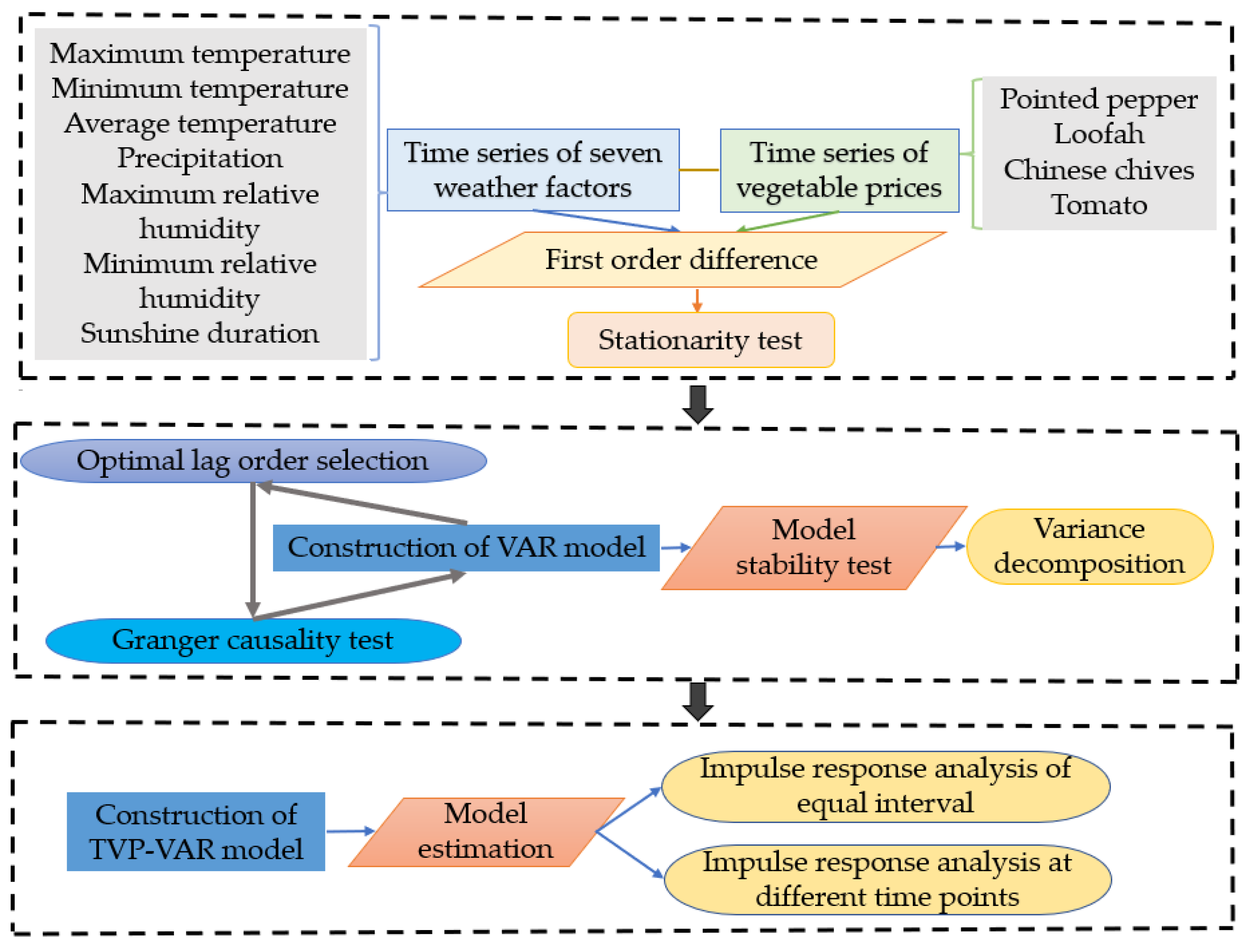
Figure 1. Experimental flowchart.
Agronomy 12 02680 g001
Figure 2. Sample autocorrelation, sample path and posterior density diagrams of the pointed pepper analysis unit.
Agronomy 12 02680 g002
Figure 3. Equal-interval impulse response in the pointed pepper analysis unit. ε   = positive shocks of one-unit standard deviation; PPP = D pointed pepper price; MAT = D maximum temperature; MIT = D minimum temperature; AT = D average temperature; PR = D precipitation.
Agronomy 12 02680 g003
Figure 4. Impulse response at different time points in the pointed pepper analysis unit. ε   = positive shocks of one-unit standard deviation; PPP = D pointed pepper price; MAT = D maximum temperature; MIT = D minimum temperature; AT = D average temperature; PR = D precipitation.
Agronomy 12 02680 g004
Table 1. Descriptive statistics of the vegetable prices. PPP = D pointed pepper price; LP = D loofah price; CCP = D Chinese chives price; TP = D Tomato price; Std. Dev. = standard deviation; C.V. = coefficient of variation.
D Pointed
Pepper Price (PPP)
D Loofah
Price (LP)
D Chinese Chives Price (CCP)D Tomato
Price (TP)
Mean0.020 0.006 0.007 0.011
Median−0.001 0.003 0.042 0.023
Maximum2.583 5.451 2.154 1.453
Minimum−1.920 −3.624 −1.967 −1.186
Std. Dev.0.602 0.906 0.460 0.392
C.V.30.115165.71435.636
Observations215215215215
Table 2. Descriptive statistics of the weather factors. MAT = D maximum temperature; MIT = D minimum temperature; AT = D average temperature; PR = D precipitation; MARH = D maximum relative humidity; MIRH = D minimum relative humidity; SD = D sunshine duration; Sg = Shouguang County; Cl = Changle County.
D Maximum
Temperature (MAT)
D Minimum
Temperature (MIT)
D Average
Temperature (AT)
D Precipitation (PR)D Maximum
Relative
Humidity (MARH)
D Minimum
Relative
Humidity (MIRH)
D Sunshine
Duration (SD)
SgClSgClSgClSgClSgClSgClSgCl
Mean−0.018−0.018−0.038−0.041−0.027−0.028−0.073−0.1440.001−0.007−0.114−0.119−0.057−0.056
Median−0.264−0.2430.0710.143−0.268−0.2850.0000.0000.5710.143−0.857−0.714−0.160−0.117
Maximum12.28911.8147.42110.66410.20711.041296.300414.80028.85722.71437.64338.9296.8483.960
Minimum−10.771−10.829−7.729−8.368−8.514−9.745−252.700−408.000−30.250−29.893−29.045−37.375−4.898−3.510
Std. Dev.3.5903.6822.5212.8672.8543.02341.65357.7138.6268.12711.97412.1441.7171.619
C.V.−199.444−204.556−66.342−69.927−105.704−107.964−570.589−400.7858626−1161−105.035−102.05−30.123−28.911
Observations215215215215215215215215215215215215215215
Table 3. Granger causality test.
Analysis UnitsThe Null HypothesisLagp-ValueConclusion
Pointed pepperMAT does not Granger Cause PPPLag 30.0402 **Reject
MIT does not Granger Cause PPPLag 30.0218 **Reject
AT does not Granger Cause PPPLag 30.0392 **Reject
PR does not Granger Cause PPPLag 30.001 ***Reject
LoofahMAT does not Granger Cause LPLag 50.0056 ***Reject
AT does not Granger Cause LPLag 50.0347 **Reject
MIRH does not Granger Cause LPLag 50.0232 **Reject
SD does not Granger Cause LPLag 50.0026 ***Reject
Chinese chivesMAT does not Granger Cause CCPLag 40.0003 ***Reject
AT does not Granger Cause CCPLag 40.0003 ***Reject
TomatoMAT does not Granger Cause TPLag 80.0091 ***Reject
AT does not Granger Cause TPLag 80.0129 **Reject
SD does not Granger Cause TPLag 80.0158 **Reject
*** and ** indicate the statistical significance at the 1% and 5% levels, respectively.
Table 4. Variance decompositions of pointed pepper price fluctuations.
PeriodMATMITATPRPPP
10.0258821.2780850.4815571.98872296.22575
20.3193461.7840590.5384602.43958094.91855
31.8173164.2277250.5357145.88664087.53260
42.0271294.2322330.5321546.28792886.92056
52.3086904.5506470.5286866.26827086.34371
62.3047004.5468590.548226.41114486.18908
72.3287184.5695120.5564276.41799286.12735
82.3289974.5691920.5597676.42417286.11787
92.3330074.5688180.5598536.43450386.10382
102.3335314.5687890.5598686.43486186.10295
Table 5. Variance decompositions of loofah price fluctuations.
PeriodMATATMIRHSDLP
12.0927741.4737400.6046650.44818495.38064
27.4347452.3105421.8764401.40275586.97552
37.3614102.2318382.0646321.50765986.83446
47.8318182.1753882.2834572.02155485.68778
57.8017712.2250182.2762712.34014985.35679
67.8259302.2188322.2742042.48081685.20022
77.8420012.2147672.2711802.63305085.03900
87.8323832.2129092.2710982.73919484.94442
97.8261152.2123922.2710322.82292284.86754
107.8233462.2114142.2699192.88152784.81379
Table 6. Variance decompositions of Chinese chives price fluctuations.
PeriodMATATCCP
11.6315790.09992098.26850
27.8782120.80008491.32170
310.392011.02473088.58326
410.412371.04812588.53950
510.529681.05655588.41377
610.529461.06317288.40736
710.532771.06847788.39875
810.532771.06909988.39813
910.533541.06927588.39718
1010.533611.06930488.39709
Table 7. Variance decompositions of tomato price fluctuations.
PeriodMATATSDTP
10.0161320.9059240.00000099.07794
20.4114800.8997180.00260698.68620
33.0783740.8763550.42845595.61682
43.1926020.9367081.46621994.40447
53.1806351.0266502.62742593.16529
63.1772321.0229403.21317392.58666
73.1807371.0174733.74349692.05829
83.1711621.0187264.14127791.66883
93.1719391.0183434.46457791.34514
103.1706651.0168334.71390391.09860
Table 8. TVP-VAR model estimation results of the pointed pepper analysis unit. Mean = posterior distribution mean; Std. Dev. = standard deviation; 95% L = lower limitation of the 95% confidence interval; 95% U = upper limitation of the 95% confidence interval (95% U); G. C. D. = Geweke convergence diagnostic; I. F. = invalid factor.
ParameterMeanStd. Dev.95% L95% UG. C. D.I. F.
β 1 0.00230.00030.00180.00280.45916.68
β 2 0.00230.00030.00180.00290.2269.47
α 1 0.00520.00130.00330.00840.13333.21
α 2 0.00500.00130.00320.00830.21237.49
h 1 0.00590.00200.00340.01070.95274.2
h 2 0.00550.00150.00340.00920.01566.81
Note: TVP-VAR model (Lag = 3) Iteration: 10,000 Sigma ( β ): Diagonal.
Table 9. Information summary for the TVP-VAR models of the four analysis units.
Analysis UnitsVariablesOptimal
Lag Order
IntervalsTime Points
Dependent VariableIndependent
Variables
Pointed PepperPPPMAT, MIT, AT, PR32, 3, 6106th, 122nd, 157th, 195th
LoofahLPMAT, AT, MIRH, SD52, 4, 686th, 122nd, 159th, 195th
Chinese chivesCCPMAT, AT42, 3, 628th, 86th, 122nd, 195th
TomatoTPMAT, AT, SD81, 3, 686th, 122nd, 185th, 195th
Publisher’s Note: MDPI stays neutral with regard to jurisdictional claims in published maps and institutional affiliations.