Article

Estimating Tomato Transpiration Cultivated in a Sunken Solar Greenhouse with the Penman-Monteith, Shuttleworth-Wallace and Priestley-Taylor Models in the North China Plain

1
Beijing Key Laboratory of Urban Hydrological Cycle and Sponge City Technology, College of Water Sciences, Beijing Normal University, Beijing 100875, China
2
PowerChina Zhongnan Engineering Corporation Limited, Changsha 410014, China
*
Author to whom correspondence should be addressed.
Agronomy 2022, 12(10), 2382; https://doi.org/10.3390/agronomy12102382
Submission received: 31 August 2022 / Revised: 21 September 2022 / Accepted: 28 September 2022 / Published: 1 October 2022
(This article belongs to the Section Water Use and Irrigation)

Abstract

:
Tomato crops are increasingly cultivated in winter in solar greenhouses to achieve high economic benefit in the North China Plain (NCP). Accurate predictions of crop transpiration (Tr) are of great significance for formulating a scientific irrigation system and increasing water productivity in this water shortage region. In this study, tomato transpiration at daily and hourly scales were estimated using Penman-Monteith (PM), Shuttleworth-Wallace (SW), and Priestley-Taylor (PT) models, and results were compared to the measured sap flow data (SF) in three tomato growth seasons in winter from 1 November 2018 to 9 December 2020. Results showed that both PM and SW models could perfectly estimate daily tomato Tr, with a determination coefficient R2 of 0.96 and 0.94 and slopes of 0.99 and 0.98, respectively, when all three seasons’ data were pooled together. The estimated daily Tr by the original PT model with a coefficient (α) of 1.26 was also linearly related to the SF with R2 of 0.92; however, the Tr was underestimated by 33%. Then α was calibrated using the data in the 2018 winter season. When the calibrated α was used in the 2019 and 2020 seasons, the estimated daily Tr showed comparable results with the PM and SW models. At hourly scales, the PM model performed best with an error of 3.0%, followed by the PT model (7.8%); the SW model underestimated Tr by 18.2%. In conclusion, all three models could be used to estimate daily Tr, and the PM and calculated PT models can be used to estimate hourly Tr.

1. Introduction

Greenhouse cultivation, as a representative of controlled environmental agriculture, has become popular in all corners of the world [1]. Growers enjoy great advantages from greenhouse farming, including saving energy, extending the growing season, and planting under undesirable climatic conditions. The North China Plain (NCP) is one of the largest regions for grain and vegetable production in China. The total vegetable production and planting area in 2020 in the NCP accounted for 28.9% and 19.2% of China’s total vegetable production and planting area, respectively [2]. In the NCP, solar greenhouses, especially sunken solar greenhouses (SSG) with a thicker back wall and 1.0–2.0 m deep soil surface, are now extensively used in the winter season. This modified structure in SSG increases the greenhouse thermal insulation capacity, consequently providing a more suitable environment for crops even in the coldest winter months [3,4].
Irrigation water in agriculture accounts for 61.2% of water use in China and places high pressure on water use in the NCP, where water resources account for approximately 3−4% of China’s total amount [5]. Traditional irrigation mode with surface irrigation in greenhouses generally uses a lot of water [6,7]. This model has been found to result in low water use efficiency (~30–50%) and a high potential for water resource pollution through nitrogen and phosphorous leaching [8]. With the advanced irrigation technologies (i.e., drip irrigation, fertigation system) being used in greenhouses for improving plant growth and achieving a high yield and good quality, optimized irrigation scheduling (including irrigation timing, amount, and frequency) could help growers save water and improve income [6,9,10]. Tomatoes are one of the most popular fruits and vegetables in the world, as well as in China, and are widely grown in the greenhouses in the NCP to fulfill the demand outside of the growing season. Optimized water supply is one of the main factors in achieving high yields and good quality greenhouse tomatoes [11,12,13].
Crop transpiration (Tr), which is an important part of the soil-vegetation-atmosphere continuum system [14], accounts for approximately 65–70% of total seasonal evapotranspiration and up to 90% during vigorous growth periods or under full cover conditions [15,16,17]. In greenhouses, the soil surface is always covered by a plastic sheet to reduce soil evaporation and provide a comfortable environment for field management. In this situation, crop transpiration can be roughly regarded as crop evapotranspiration. Thus, the accurate prediction of crop transpiration is of great significance for formulating scientific irrigation scheduling and developing water-saving agriculture.
Crop transpiration can be evaluated by two different approaches: instruments and mathematical models. Instruments, including lysimeters [18,19], sap flow [20,21], Bowen [22], and Eddy covariance methods [23], are usually expensive and limited by temporal and spatial factors. Mathematical models can be conveniently applied to a wide range of situations. Thus, in recent decades, many models have been developed for crop transpiration estimation. The prevailing models for predicting evapotranspiration and transpiration include the Penman-Monteith (PM) [17], Shuttleworth-Wallace (SW) [24], and Priestley-Taylor (PT) models [25]. These three models have been applied to a wide variety of crops, such as tomatoes [26], cucumbers [27], baby pak choi [28], and grapevines [29]. The PM method has been used to model cherry orchard transpiration in northern China, in which parameter values were estimated by the Bayesian method [30]. In greenhouses with revised canopy resistance, the PM model also performed well for Tr estimation for Gerbera and cucumber crops [31,32], though cucumber Tr was overestimated by 7.35% in spring and autumn [32].
The SW model can distinguish crop Tr and soil evaporation [24]. Hence, it has been widely applied in full and sparse canopy conditions in agricultural and forest ecosystems [33]. By using the calibrated model parameters, the SW model has been successfully used in the sparse vegetation canopy of a vineyard in an arid area [34], maize evapotranspiration with plastic-film mulching soil surface [35], and cucumbers transpiration in Venlo-type greenhouses [27]. The PT model was first developed to estimate water evaporation from a horizontally uniform saturated surface (i.e., water surface or saturated canopy surface after heavy rainfall) [25]. For drying land surface, the Priestley and Taylor coefficient (α) should be validated based on sites, climatic environment, and crops [36,37]. With a revised α, the PT model has been successfully used in a rice-wheat rotation system [38] and evapotranspiration of tomatoes in a greenhouse [39].
The SSG is a newly developed solar greenhouse type with high isolation conditions and a great heating effect; therefore, it has been increasingly used in the NCP [3,4]. The PM, SW, and PT models have been found generally perform well when appropriate parameters were calibrated. However, their suitability should be further evaluated in these newly developed greenhouses.
Therefore, a three-winters long experiment was conducted in a commercial SSG with tomato cultivation in the NCP. The objectives of this study were to (1) evaluate the Penman-Monteith, Shuttleworth-Wallace, and Priestley-Taylor (PT) models for estimating tomato transpiration (on daily and hourly scales) based on the measured sap flow data in the sunken solar greenhouse and (2) conduct a sensitivity analysis to qualify the parameters’ variation on model results and finally optimize parameters for each model.

2. Materials and Methods

2.1. Experimental Site

The experiment was conducted over three winters, from November 2018 to December 2020, in a commercial sunken solar greenhouse (SSG) located at Dacaozhuang National Breeding Experimental Station, Ningjin County, Hebei Province, China (37°30′6″ N, 114°57′22″ E, 26 m above the sea level). The experiment area is an important fruit and vegetable producing region in the North China Plain. The climate in the study region belongs to a typical temperate continental monsoon climate. The annual mean temperature is 12–14 °C, the annual average wind speed is 2.33 m s−1, and the total yearly sunshine duration is 2538 h. The average annual rainfall is 483 mm, of which approximately 60–70% distributes during the rainy season from July to September. The soil type in the upper 40 cm soil layer is silty loam with a mean bulk density of 1.40 g cm−3, the wilting point water content is 0.22 cm3 cm−3, and the field soil water capacity is 0.40 cm3 cm−3. The SSG with tomato crops is in an east-west orientation and covers an area of 1660 m2 with inside dimensions of 10 m in width and 166 m in length (Figure 1). The roof of the greenhouse is covered with 0.1 mm-thick polyethylene film. A rolled straw curtain was placed on the top of the roof from 17:00 to 09:00 the next day in winter to reduce heat loss. The soil surface was 1m lower than the outside, and the north-facing rear wall was much thicker (the thickness of the bottom and top is 5.0 m and 1.2 m, respectively). This structure reduces heat loss and stores more heat in winter. Detailed information on the SSG can be found in the paper by Yang et al. [3].

2.2. Planting and Management

The tomato seedlings were transplanted on ridges after they had four leaves. Tomatoes were planted in the single ridge and double rows mode. The ridge measured 9 m in length, 1 m on the surface width, and 0.15–0.20 m in height. The distance between ridges was 0.4 m, the row spacing on the ridge was 0.5 m, and the tomato plant spacing was 0.4 m, with an average of 45 plants per ridge. Tomato management was done by farmers following local practices. Stems above the fifth fruit branch were pruned when the fifth branch fruit was flowering. Leaves in the lower part of the stem were pruned in the late tomato growth stage to enhance underlayer ventilation and reduce nutrition uptake. Fertilizer application included base and topdressing fertilization. The base fertilizer was compounded and manually spread before ridging. Soluble compound fertilizer was used for topdressing at different times during the tomato growth period. Fertilization details are summarized in Table 1.
A drip irrigation system was installed to irrigate tomatoes in this experiment. Drip tapes (Hebei Runtian Water-Saving Equipment Co., Ltd., Shijiazhuang, China) were deployed parallel to the crop rows, with one tape (16 mm in diameter; 2.5 L h−1 under working pressure 0.1 mPa; 40 cm in dripper spacing) per row. Irrigation was guided by the soil matrix potential (SMP) and measured using dial-type tensiometers (Beijing Waterstar Tech Co., Ltd., Beijing, China) installed under the drippers at a depth of 20 cm in the soil (Figure 1c). Three tensiometers were deployed in the field. When the two SMPs of the three reached the target value of −35 kPa, irrigation started. Irrigation details are shown in Table 2. In practice, irrigation started when the SMP was higher than −35 kPa because the farmer of this SSG was busy and wanted to finish irrigation in advance and then do other things. Therefore, the SMPs in the three seasons were higher than −35 kPa, indicating sufficient soil water condition.

2.3. Measurements

The microclimate inside was measured in the three winter seasons. Variables of net radiation, air temperature, relative humidity, and air speed were simultaneously measured with a meteorological station deployed in the middle of the greenhouse (Figure 1d). The corresponding sensors deployed at 2 m height were listed as follows: net radiometer (Model TBQ-2, Jinzhou Sunshine Technology Co., Ltd., Jinzhou, China), temperature and relative humidity recorder (Model VP-4, METER Group, Inc., Pullman, WA, USA), and air velocity meter (two-dimensional ultrasonic anemometer ATMOS 22, METER Group, Inc., Pullman, WA, USA), respectively. The data logger was used to sample data at 1 min intervals and store data every 30 min. One set of sap flow gauges (Flow32-1K, Campbell Scientific, Logan, UT, USA) was installed on eight sample plants of similar growth conditions, which were selected from the center of the experimental greenhouse. Eight representative tomato plants with similar growth parameters were selected in the middle of the experimental site. Sap flow gauges were approximately 15 cm above the ground (Figure 1e), sampled every 1 min with a CR1000 data logger (Campbell Scientific, Logan, UT, USA), and the accumulated data was stored for 30 min. Plant height and leaf area were measured once a month using three labeled plants. Leaf area (LA) was calculated using the leaf length (L) and width (W) with an in situ calibrated regression LA = 0.38L × W. The leaf area index (LAI) was calculated using the mean leaf area of a plant and the mean soil surface area occupied by a plant as L A I = i = 1 n L A i / S , where n is the total number of leaves in a plant and S is the mean soil surface area occupied by a plant. Marketable fresh tomato yield in the SSG was recorded at each sale. The total yield was the sum of all sales in a season and was finally converted into a unit area (ha).

3. Models and Parameters

In this study, three classical methods, the Penman-Monteith (PM), Shuttleworth-Wallace model (SW), and Priestley–Taylor (PT) models, for crop transpiration estimation were evaluated for estimating tomato plants’ transpiration in the SSG. Each method was described in detail as follows.

3.1. Penman-Monteith Model

Penman and Monteith comprehensively combined the canopy water vapor transport process and the energy balance equation for calculating crop transpiration. The PM model is based on the big leaf theory and considers the whole canopy as a one-layer source [17]. The PM model has been widely used for various crops and is expressed as
λ T r = Δ R n c + 24 × 3600 × ρ a c p e s e a r a Δ + γ ( 1 + r c r a )
where T r is the transpiration rate (mm d−1), λ is the latent heat of vaporization (=2.45 MJ kg−1), Δ is the slope of the saturation vapor pressure versus temperature curve (kPa C−1),   R n c is the net radiation intercepted by the canopy (MJ m−2 day−1), ρ a is the air density (kg m−3), c p is the specific heat at constant pressure (=1.013 × 10⁻³ MJ kg−1 °C−1), e s is the saturation of vapor pressure at air temperature (kPa), e a is the actual vapor pressure (kPa), γ is the psychrometric constant (kPa °C−1), r a is the aerodynamic resistance (s m−1), and r c is the canopy resistance (s m−1).   R n c can be calculated by the measured net radiation R n and the net radiation at the substrate surface R n s using a Beer’s law relationship in the form of:
R n c = R n R n s
R n s = R n exp ( C L A I )
where C is the extinction coefficient, chosen as 0.8 in our study. LAI is the leaf area index.
The PM model assumes that the aerodynamic resistance r a is inversely proportional to wind speed and changes with the plant height. However, the wind speed in the greenhouse was much lower than that outside, even occasionally close to 0. In this case, r a will be close to infinite, which is inconsistent with the actual situation. Therefore, the modified method proposed by Thom and Oliver was introduced to calculate r a in the greenhouse [40]. The formula is as follows:
r a = 4.72 [ ln ( x d Z 0 ) ] 2 ( 1 + 0.54 u 2 )
where x is the height of wind measurements (2 m in this study), d is the zero-plane displacement height (m) calculated as 0.64 times the crop height. Z 0 is the crop roughness length (m) taken as 0.13 times crop height and u 2 is the wind speed at 2 m height (m s−1).
The canopy resistance r c is related to the leaf area index and environmental factors. The Jarvis method was recommended for estimating and is as follows:
r c = r S T m i n L A I e i F i ( X i )
where r S T m i n is the minimal stomatal resistance. The stomatal conductance data in this experiment were few, so the minimal stomatal resistance r S T m i n was set as 33.5 s m−1 according to the research of Gong et al. [41]. L A I e is the active (sunlit) leaf area index which is calculated as equal to the actual LAI when LAI ≤ 2, 0.5LAI when LAI ≥ 3, and 2 for an intermediate LAI. In this study, LAI varied between 1.55 and 3.27 during selected periods, including all three assumptions above. F i ( X i ) is the environmental stress function and ranges from 0 to 1, where X i is the environmental factors, generally including the net radiation R n (W m−2), vapor pressure deficit (VPD = ( e s e a ), kPa) and air temperature T (°C) [42,43]. Each stress function was shown as follows:
F 1 = d 0 R n c + R n
F 2 = 1 0.238 V P D
F 3 = 1 1.6 × 10 3 ( 25 T a ) 2   ( 0 C < T a < 25 C )
where c equals 400 for crops and d 0   = 1 + c/1000 according to the study of Zhou et al. When the air temperature was higher than 25 °C, F3 was considered as 1 [44].

3.2. Shuttleworth-Wallace Model

Shuttleworth and Wallace established a dual-source evapotranspiration model based on the PM model without ignoring the soil evaporation and assuming that the canopy is uniformly covered [24]. The dual source represents soil evaporation and crop canopy transpiration. The transpiration term is calculated as follows:
λ T r = C c × P M c
P M c = Δ A + [ ( 24 × 3600 ) ρ c p V P D Δ r a c A s ] ( r a a + r a c ) Δ + γ [ 1 + r s c ( r a a + r a c ) ]
C c = 1 1 + ( R c R a ) [ R s ( R c + R a ) ]
where C c is the weighting coefficient, A and A s are the available energy to the canopy and soil surface which can be taken as A = R n G and A s = R n s G , G is the soil heat flux (MJ m−2 d−1), r a a is the aerodynamic resistance between the canopy source height and reference level (s m−1), r a c is the bulk boundary layer resistance of the canopy (s m−1), r a s is the aerodynamic resistance between the soil and canopy source height (s m−1), r s c is the bulk stomatal resistance of the canopy (s m−1), and r s s is the soil surface resistance (s m−1). R a , R c and R s are given by the expressions:
R a = ( Δ + γ ) r a a
R c = ( Δ + γ ) r a c + γ r s c
R s = ( Δ + γ ) r a s + γ r s s

3.2.1. Aerodynamic Resistances

Shuttleworth and Wallace set two limit values: the fully developed crop (LAI > 4) and the bare soil (LAI = 0), which can be given by:
r a a ( 0 ) = ln ( x z 0 ) ln ( x z 0 ) u κ 2 r a s ( 0 )   ( LAI > 4 )
r a s ( 0 ) = ln ( x z 0 ) ln { ( d + z 0 ) z 0 } u κ 2   ( LAI > 4 )
r a a ( α ) = ln ( x d z 0 ) u κ 2 [ ln { ( x d ) ( h d ) } + h n ( h d ) × [ exp [ n ( 1 ( d + z 0 ) h ) ] 1 ] ] ( LAI = 0 )
r a s ( α ) = ln ( x d z 0 ) u κ 2 h n ( h d ) [ exp n exp [ n ( 1 ( d + z 0 ) h ) ] ]   ( LAI = 0 )
In other cases, the r a a and r a s are assumed to be in a linear relationship between their asymptotic limits based on LAI. It is expressed in the form
r a a = LAI r a a ( α ) 4 + ( 4 LAI ) r a a ( 0 ) 4 ( 0 LAI 4 )
r a s = LAI r a s ( α ) 4 + ( 4 LAI ) r a s ( 0 ) 4 ( 0 LAI 4 )
where κ is von Kármán’s constant (=0.41), n is the eddy diffusion coefficient (=2.54), h is the crop height (m), z 0 is the soil’s effective roughness length, taken as 0.01 m. x is the reference height (=2 m), d is the zero-plane displacement height (m), calculated as 0.64 times crop height. Z 0 is the crop roughness length (m), taken as 0.13 times crop height and u is the wind speed at the reference height.

3.2.2. Bulk Stomatal and Boundary Layer Resistances

The canopy resistance r s c , known as surface resistances, is the emblem of the stomatal behavior of the entire crop. It is written as:
r s c = r S T 2 L A I
r S T = 82 [ R n / 2 L A I + 4.30 R n / 2 L A I + 0.54 ] × ( 1 + 0.023 × ( T a 24.5 ) 2 )
where r S T is the mean stomatal resistance of amphistomatous leaves and was calculated by environment and crop factors [26]; R n is the net radiation above the canopy (W m−2), Ta is the air temperature (°C), and LAI is the leaf area index.
Shuttleworth and Wallace believed that the bulk boundary layer resistance of canopy r a c , like r s c , belonged to the surface resistance. It inversely varies with the total leaf area of the crop and is calculated as:
r a c = r b 2 L A I
r b = ( 100 / n ) ( w u h ) 1 2 [ 1 exp ( n 2 ) ] 1
w = w m a x [ 1 exp ( 0.6 L A I ) ]
where r b is the mean boundary layer resistance (s m−1), w is the typical leaf width (m) for the annual crop, it can be calculated by maximum crop leaf width ( w m a x ) [44]. u h is the wind speed at the top of the canopy (s m−1), n is the eddy diffusivity decay constant (=2.54 in this study).

3.2.3. Soil Surface Resistance

Soil surface resistance r s s is the main factor affecting soil evaporation, but simultaneously it has little effect on crop transpiration. Anadranistakis indicated a strong correlation between soil surface resistance and soil moisture content. Its expression is shown as:
r s s = r s m i n s [ 2.5 ( θ s θ g ) 1.5 ]
where r s m i n s is the minimum soil surface resistance (=100 s m−1), θ s is the surface soil water content at field capacity (=0.40 m3 m−3), and θ g is the soil water content for the surface soil layer (0–20 cm).

3.3. Priestley-Taylor Model

Priestley and Taylor eliminated aerodynamic resistance and used the net radiation to calculate the evapotranspiration and transpiration [25]. This method is simple and convenient due to its fewer input parameters, and expressed as follows:
λ T r = 1 λ Δ Δ + γ R n ( 1 e C L A I )
α m = exp [ ( T a T o p t 1 ) 2 ] × V P D a × b u
Considering the large deviation between estimated daily transpiration and SF, the coefficient α was calibrated (denoted as α m in Equation (28)) using air temperature, the optimal temperature for crop growth (Topt), VPD, and wind speed in the 2018 winter season. The parameter calibration process was described as follows: data from the 77 days in the 2018 winter season were used, and goal was the minimum MAE, the process was to finally solve, using the ’SOLVER’ function in the Excel 2018, the calibrated coefficients a and b in the PT model, which were 0.71 and 13.29, respectively. The optimal temperature for tomato crops (Topt) was 26 °C for greenhouse tomatoes [43]. Then the regulated α m was used to estimate the daily transpiration in the 2019 and 2020 winter seasons.

3.4. Evaluation of Model Performance

The evaluation of the model performance was mainly based on the linear correlation between the predicted value ( P i ) and the observed value ( O i ). The coefficient of mean absolute error (MAE), root mean square error (RSME), index of agreement ( d I A ), Nash-Sutcliffe efficiency (NSE), and RMSE observation standard deviation ratio (RSR) were also recommended for use. They were computed as follows:
M A E = i = 1 N | P i Q i | N
R M S E = i = 1 N ( P i Q i ) 2 N
d I A = 1 i = 1 N ( P i Q i ) 2 i = 1 N ( | P i Q ¯ | + | Q i Q ¯ | ) 2
N S E = 1 i = 1 N ( Q i P i ) 2 i = 1 N ( Q i Q ¯ ) 2
R S R = i = 1 N ( Q i P i ) 2 i = 1 N ( Q i Q ¯ ) 2
where P i ¯ is the average of the predicted value,   O i ¯ is the average of the observed value, N is the sample number. If the simulation performance was very good, R2 and dIA are close to 1, while MAE and RMSE are close to 0. The evaluation criteria for NSE and RSR are shown in Table 3.

3.5. Models’ Sensitivity Analysis

The accuracy of the crop transpiration estimation at both daily and hourly intervals by the PM and SW models greatly depends on the input values, which may vary with the microclimate inside and the plant characteristics. Therefore, a sensitivity analysis was performed for the PM and SW models to qualify the parameters’ variation on the uncertainty of the estimated results. The base value of the plant height (hc), leaf area index (LAI), minimum stomatal resistance (rSTmin), and extinction coefficient (C) were 1.55 m, 2.66, 33.5 s m−1, and 0.8, respectively. In the SW model, transpiration was calculated by five resistance parameters. Thus, the sensitivity analysis was conducted by changing resistance parameters. The reference values for the five resistance parameters ( r a a , r a c , r s c , r a s , r s s ) were the average values in the middle growth stage from 16 to 30 November in the 2018 winter season and set as 67, 9, 67, 574, and 168 s m−1, respectively. All parameters, including growth and resistance parameters, were adjusted at 25% intervals between −100% and 100%. Then the sensitive effect of Tr to each parameter was evaluated using the relative change of Tr with the changed parameters to the Tr estimated using the reference parameters.

3.6. Tomato Transpiration Estimation at Daily and Hourly Scale

In this study, the tomato transpiration was estimated using the PM, SW, and PT models at daily and hourly scales. At daily scale, the transpiration could be estimated using Equations (1), (9), (27), and (28). To evaluate the performance of the three models at the hourly scale, Equations (1), (9), and (27) were used by considering the unit conversion from day to hour. In Equations (1) and (10), the converter coefficient ‘24 × 3600′ (daily scale) was replaced by ‘3600′ (hourly scale). The unit of net radiation was MJ m−2 h−1, and the temperature, humidity, and vapor pressure deficit used the hourly mean values. Seven days from 4 to 10 November in the 2019 winter season were selected as representative days. During the seven days, four days were sunny (4, 5, 6, and 8 November), one day was overcast (7 November), one cloudy (9 November), and one mostly sunny (10 November). The daily average meteorological elements and tomato plant characteristics of those days are given in Table 4.

4. Results

4.1. Microclimate Conditions, Tomato Growth and Yield in the Sunken Solar Greenhouse

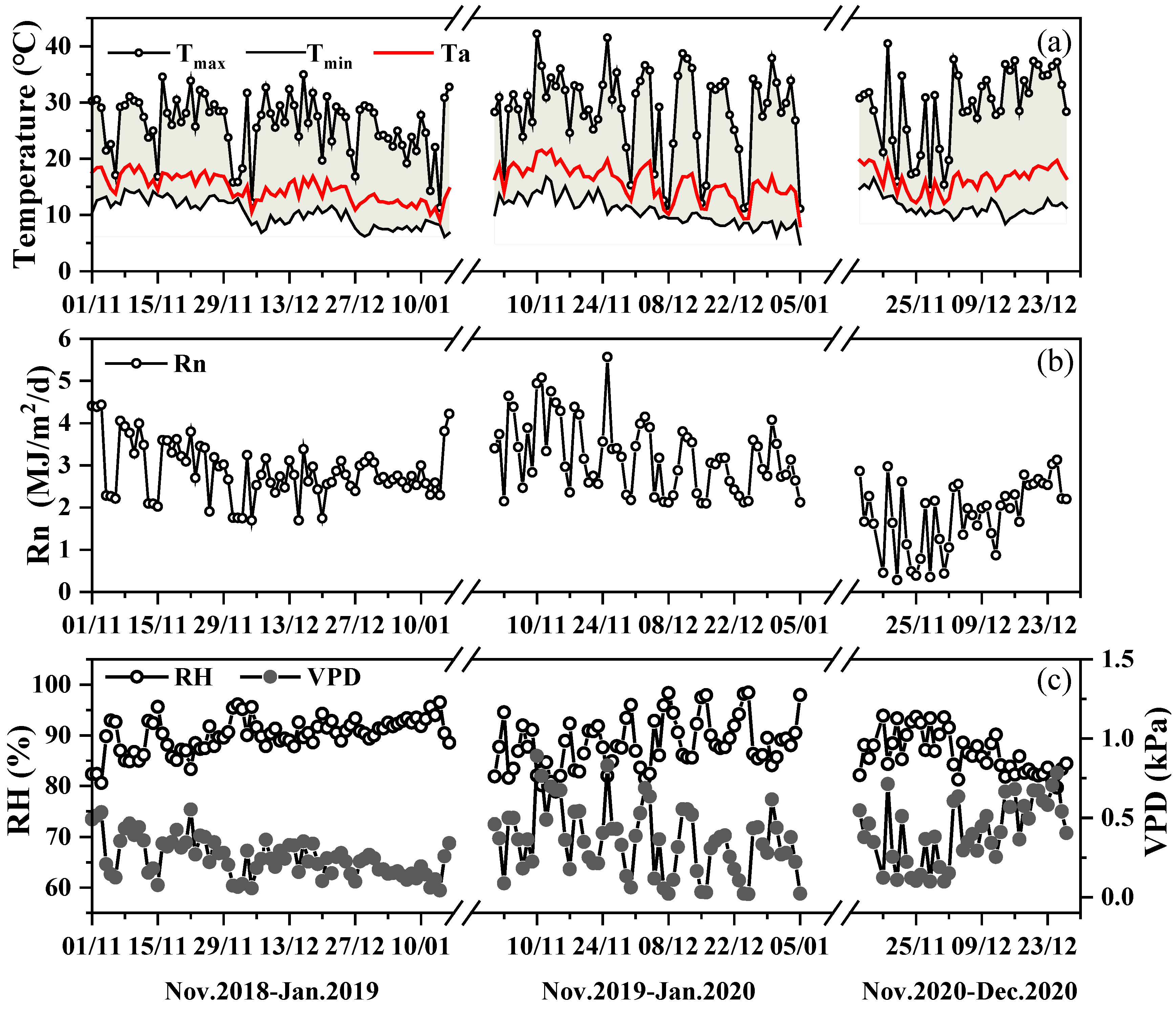
The daily mean microclimate variables inside the SSG during the three seasons are shown in Figure 2. In general, the daily temperatures in the greenhouse during the three winters ranged from 4.80 to 42.20 °C, with the daily highest temperature ranging from 10.60 to 42.20 °C (average 27.99 °C) and the lowest temperature ranging from 4.80 to 16.80 °C (average 10.80 °C). The average daily temperature of the three winters from 2018 to 2020 were 14.68, 15.82, and 16.38 °C, respectively.
The wind speed in the greenhouse was from 0.07 to 0.44 m s−1, and the daily averages during the three winters from 2018 to 2020 were 0.22, 0.29, and 0.13 m s−1, respectively. The relative humidity in the greenhouse was from 78.86 to 98.47%, and the daily averages during the three winters from 2018 to 2020 were 90.18%, 88.44%, and 86.51%. The daily average net radiation during the three winters were 2.88, 3.21, and 1.84 MJ m−2 day−1, respectively. From November to December 2020, the net radiation in the greenhouse was the smallest, which was from 0.28 to 3.13 MJ m−2 day−1. From November 2019 to January 2020, the net radiation in the greenhouse was relatively large, which was from 2.10 to 5.57 MJ m−2 day−1. The daily vapor pressure deficits were between 0.02 and 0.89 kPa, and the daily averages during the three winters from 2018 to 2020 were 0.25, 0.35, and 0.32 kPa, respectively.
During the Tr modeling period, the LAI varied between 1.55 and 3.27, and the plant height varied between 120 and 158 cm. Tomato yields were 86.5, 56.3, and 83.6ton ha−1 in the 2018, 2019, and 2020 winter seasons, respectively. These tomato yields fell into the range from 33.5 to 66.5 in the North China Plain from the published papers [46,47]. This indicated that this SSG is suitable for tomato cultivation in winter in the North China Plain.

4.2. Comparison of the Estimated Daily Transpiration and Measured Sap Flow

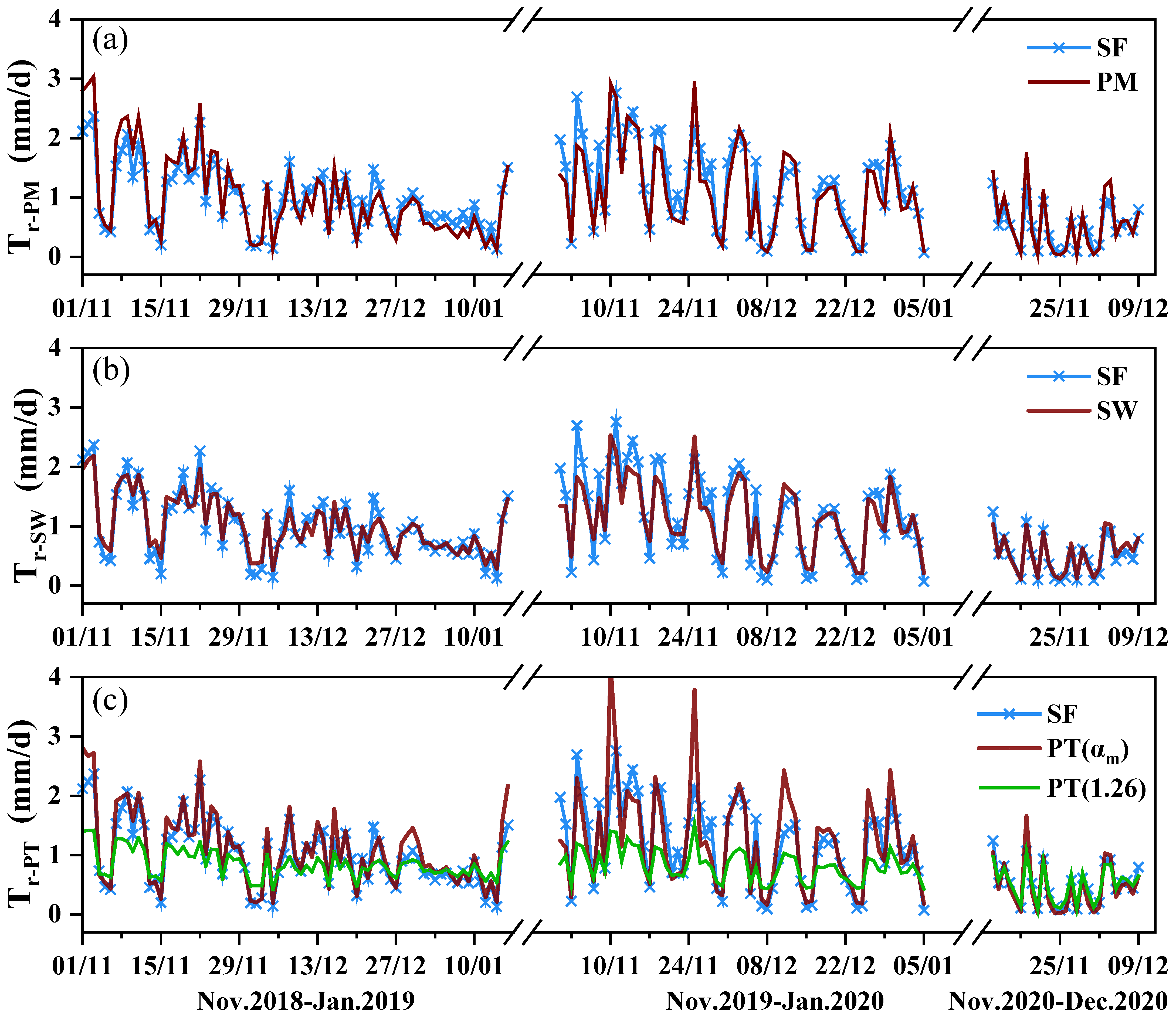
The simulated daily crop Tr by the PM, SW and PT methods and the measured daily SF amount are shown in Figure 3 and their relationships are shown in Figure 4. The results indicated that the estimated daily Tr by the PM, SW, and PT models in the three winter seasons had a strong linear correlation with the measured SF with determination coefficients R2 in the regression lines ranging from 0.91 to 0.98.
Generally, daily tomato Tr estimated using the PM model was in good agreement with the actual SF during the three winter periods when all data were pooled together, with R2 of 0.96 and the slope of the regression line was 0.99 (Figure 4d). The MAE, RMSE, and dIA were 0.18 mm d−1, 0.26 mm d−1, and 0.96, respectively. The NSE and RSR were 0.77 and 0.40, respectively, meaning the PM model performed well in general. Whereas the NSE and RSR in winter 2020 were 0.66 and 0.58, respectively, and lower than those (0.82 in NSE and 0.42–0.43 in RSR) in the previous two winters. Moreover, the PM model in general underestimated the daily Tr by 2.9% and 8.5% in the 2018 and 2019 winter seasons, respectively, while it overestimated the daily tomato transpiration by 19.4% in 2020 based on the slopes of the regression lines (Figure 4a–c).
The SW model also performed well with an R2 of 0.97 and slope of 0.93 when all data from the three seasons were pooled (Figure 4d). Compared to the PM and PT models, the MAE (0.14 mm d−1) and RMSE (0.20 mm d−1) of the SW model were at a minimum in the three winter seasons, and the dIA, NSE, and RSR were 0.97, 0.90, and 0.31, respectively. There were slight variations in the SW model evaluation parameters during the three seasons. From 2018 to 2020 winter seasons, MAE were between 0.07 and 0.22 mm d−1, RMSE between 0.09 and 0.28 mm d−1, and dIA between 0.95 and 0.98, NSE ranged from 0.85 to 0.94 and RSR from 0.25 to 0.39. Based on the slopes of the regression lines, the SW model overestimated the daily tomato transpiration by 7.5% and 2.0% in the 2018 and 2020 seasons, respectively, and underestimated it by 10.9% in the 2019 winter season.
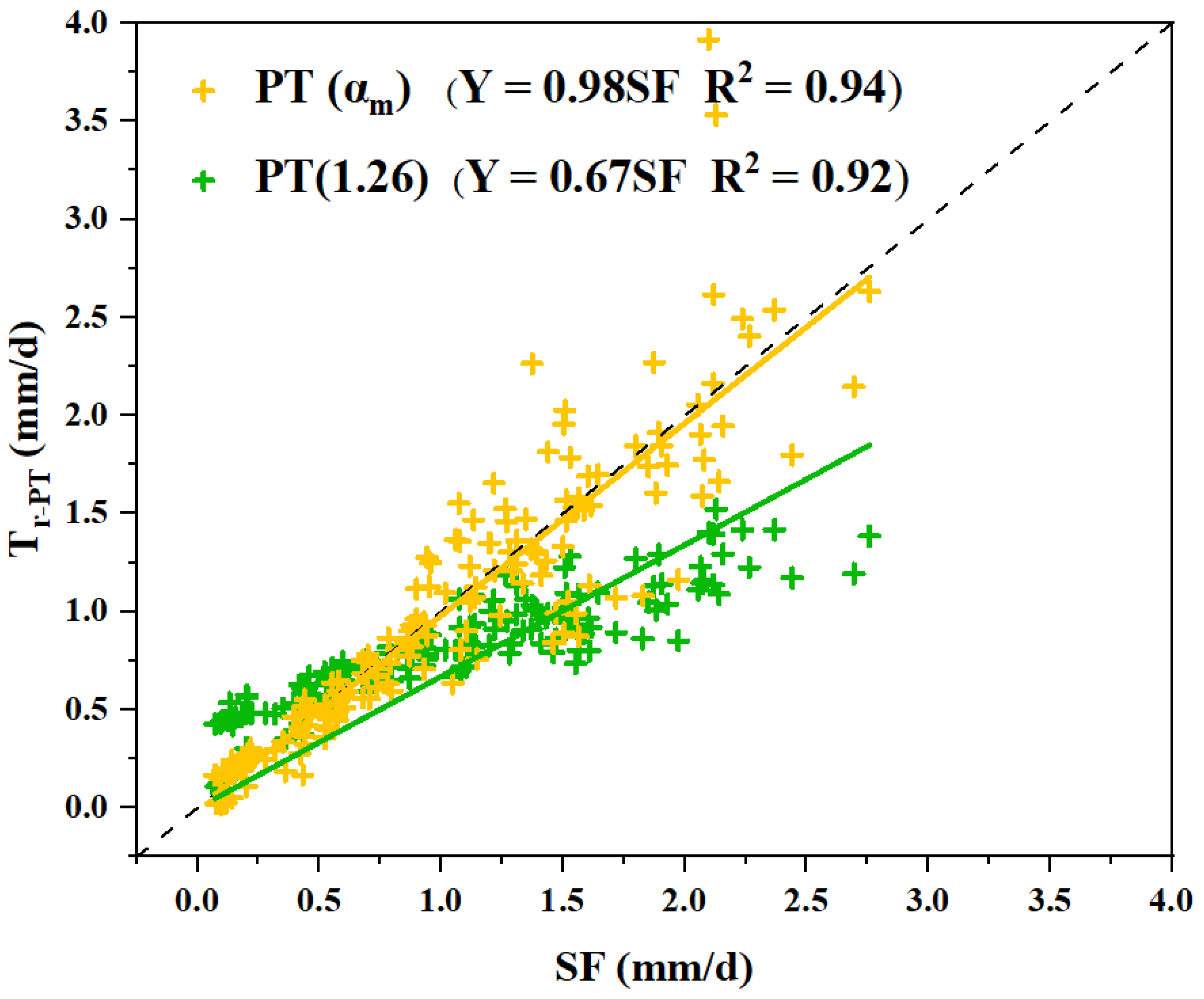
With the original α value of 1.26, the PT model underestimated the daily Tr by 33% compared with the daily SF value (Figure 5). The MAE and RSME were 0.33 and 0.46 mm d−1, respectively, and the NSE was 0.48 (unsatisfied performance at less than 0.50). Therefore, the coefficient α was calibrated using the climatic data in the 2018 season and the result is shown in Equation (28). With the calibrated α, the estimated daily Tr was strongly linearly related to SF with an R2 of 0.94 and slope of 0.98 when the three seasons’ data were pooled together (Figure 5). Then the MAE and RMSE decreased to 0.18 and 0.30 mm d−1, respectively, and the NSE increased to 0.81.

4.3. Comparison of Estimated Hourly Transpiration Rate and Measured Sap Flow

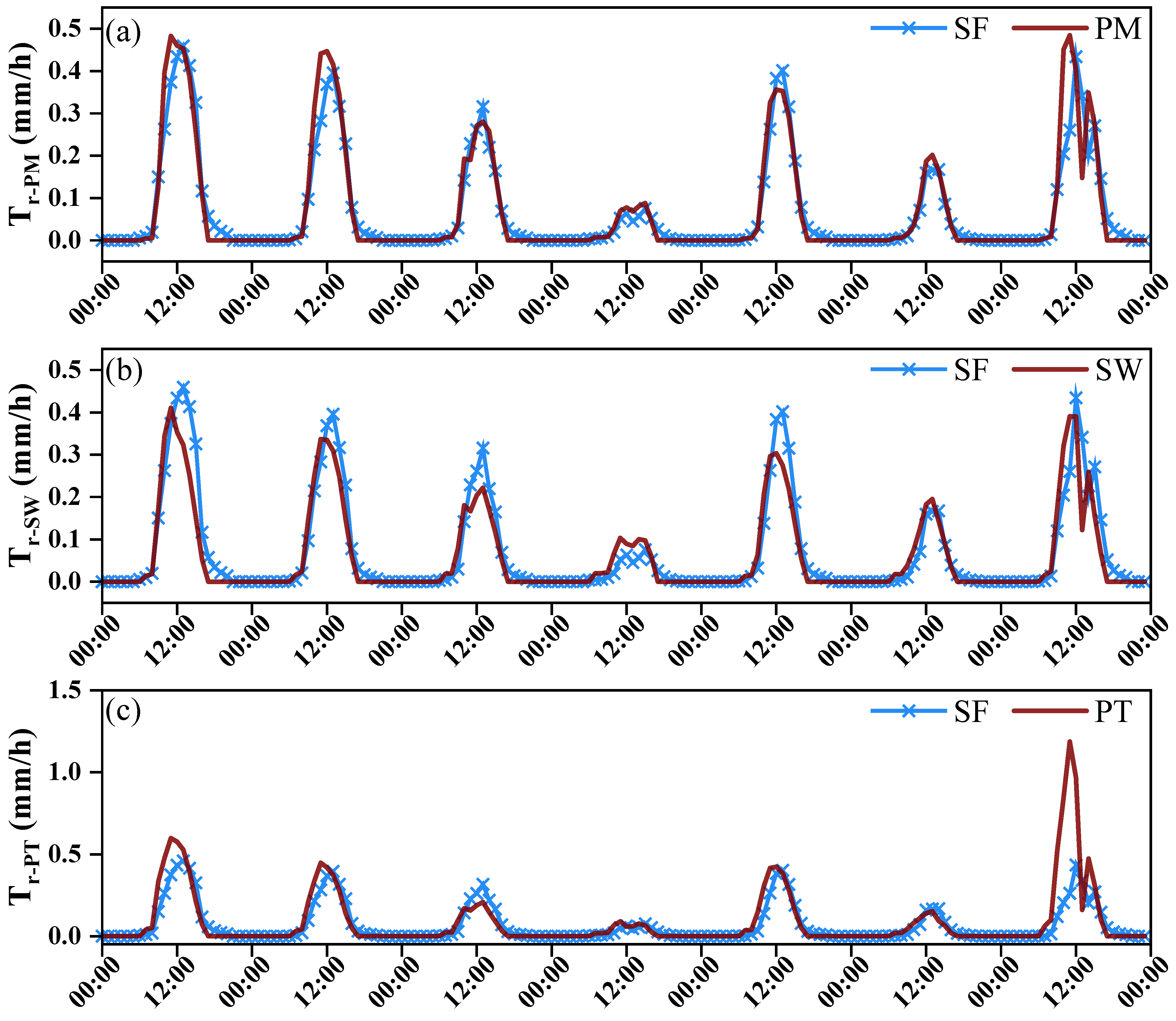
Figure 6 presents the daily courses of estimated hourly Tr rates by the three models and the measured SF in the selected seven days from 4 to 10 November 2019. It should be noted that the coefficient α was calculated using the daily average meteorological elements when the PT model was used to estimate hourly Tr. Under different weather conditions (sunny, overcast, and cloudy), the estimated hourly Tr using the PM, SW, and calibrated PT models were in good agreement with the SF. On overcast and cloudy days, both the estimated Tr and measured SF showed a multi-peak curve, while a single-peak curve was found on sunny days. However, the daily peak values of Tr and SF were not synchronized. The SF peaks were slightly delayed compared with the Tr. This appearance was much more obvious on sunny days. For example, the estimated Tr peak occurred from 11:00–12:00, while the SF peak was found at 13:00 on 5 November 2019.
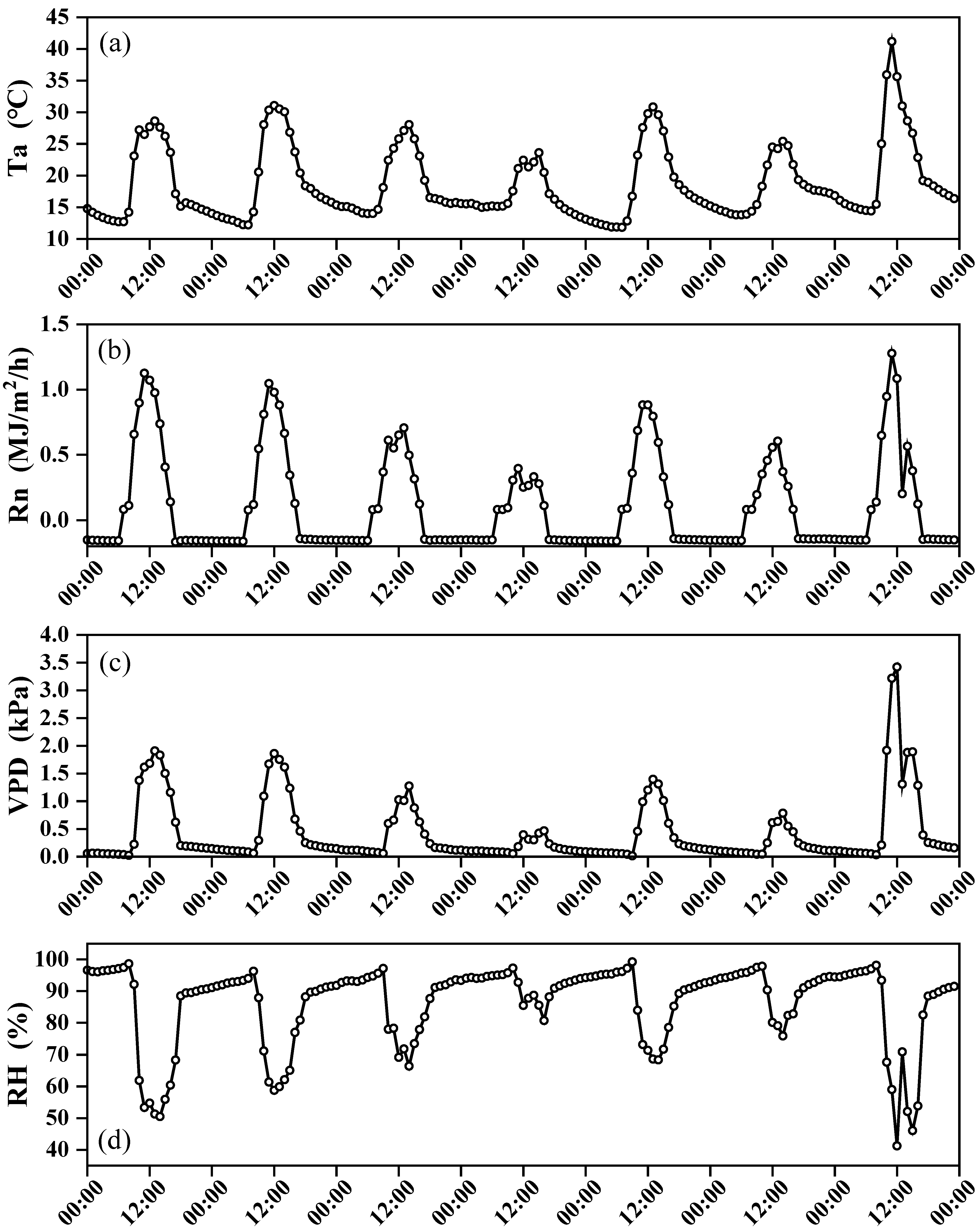
Hourly sap flow or transpiration was greatly governed by the microclimate in the greenhouse, which significantly varied under different weather conditions. The variation of meteorological conditions from 4 to 10 November 2019 is shown in Figure 7. The maximum Tr rate on 7 November (overcast day) was 0.08 mm h−1, which was 17.39% of the maximum Tr (0.46 mm h−1) on 4 November (sunny day). On 10 November, plant Tr obviously varied at noon due to the sharp change in microclimate in the SSG (Figure 7). The measured SF decreased sharply from 11:00 to 14:00, and then gradually rose from 14:00 to 15:00. The sudden shift from sunny to cloudy weather around noon on 10 November greatly reduced the incoming radiation and resulted in the air temperature greatly decreasing, which consequently caused a sharp SF decrease. With the incoming radiation increasing from 14:00–15:00, the SF also increased though the air temperature was still decreasing.
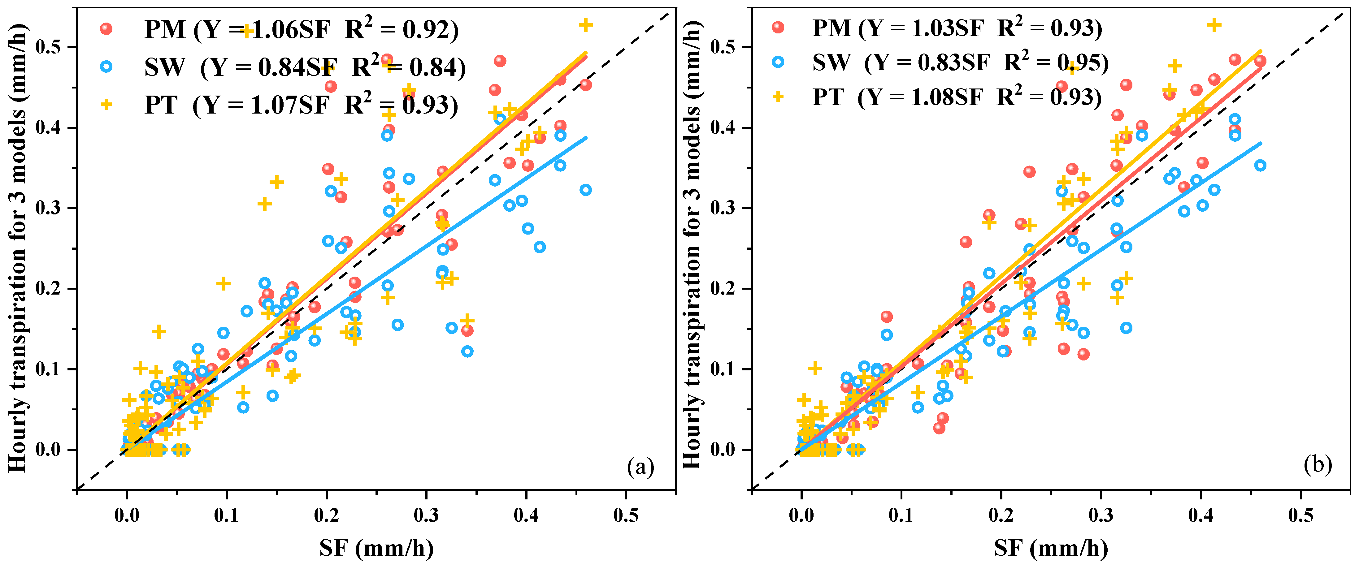
Figure 6 shows that the hourly SF clearly lagged Tr on all climatic days, especially on sunny days. The lag time was approximately 1 h. Figure 8a,b shows the relationship between estimated hourly Tr and SF when the SF lag time was not considered and considered, respectively. It can be found that most model evaluation parameters were improved when the lag time was considered. For the PM model, the slope of the regression line improved from 1.06 to 1.03, and the R2 increased from 0.92 to 0.93. For the SW model, the R2 increased from 0.84 to 0.95 though the slope slightly changed. Consideration of lag time had a slight effect on the PT model. The PM model performed well for estimating hourly Tr with a small error (3.0%). The MAE, RMSE, dIA, NSE, and RSR for the PM model were 0.02 mm h−1, 0.04 mm h−1, 0.97, 0.87, and 0.36, respectively. The PT model with the calibrated α also did well estimating Tr with an R2 of 0.93 and slope of 1.08 (Figure 8). Though the hourly Tr estimated by the SW model was strongly linearly related to SF with an R2 of 0.95. The slope of 0.83 showed the SW model underestimated the tomato Tr by approximately 17% in general.

5. Discussion

5.1. Models’ Performance at Daily Scale

The PM, SW, and PT models are generally used for crop evapotranspiration and transpiration estimation at a daily scale [29,48,49,50,51]. In this study, when all daily data in the three seasons were pooled together, the SW and PM models showed comparable results with an R2 of 0.97 and 0.96, respectively, and both were slightly better than the PT model (0.94). When the slope of the regression line was considered, both PM and PT models performed better with values of 0.99 and 0.98, respectively; however, the slope was 0.93 for the SW model, indicating an approximately 7% underestimation in general. Similarly, Federico (2012) [52] reported that the PM model performed well to estimate the transpiration of greenhouse tomatoes in autumn with about a 6% error and an R2 of 0.70. Gong’s (2020) [41] study showed that the PM model would underestimate the evapotranspiration of greenhouse tomatoes by about 10.1%; however, it was from 12.8% to 13.8% for the SW model.
The aerodynamic resistances needed to be calculated in the PM and SW models to simulate the tomato transpiration. The PM model used the formula revised by Thom and Oliver [40], which was more suitable for the low wind speed conditions in the greenhouse. In the SW model, we qualified the effect of wind speed on the estimated transpiration when the mean climatic base from 16 to 30 November in 2018 season was used, and the wind speed changed from 0.06 to 0.44 m s−1 with the amplitude change from 25% to 200% based on a mean wind of 0.22 m s−1. The results showed the variation of the simulated transpiration changed from 6% to 23%, indicating that the simulated value of transpiration would not be greatly affected within the variation range of the actual low wind speed in the greenhouse. The high R2 of 0.96 and slope of 0.93 in the regression line between estimated and measured Tr mean the SW model could be used in greenhouses under low wind conditions.
The PT coefficient α was 1.26 and was used for estimating water evaporation on a large scale [25]. However, the α greatly varied from 0.7 to 3.1 depending on climatic conditions, crop characteristics, and soil water conditions [36,53,54]. In the study, when the α value of 1.26 was used, the estimated daily transpiration was approximately 33% lower than the measured daily SF. Therefore, a modified coefficient αm, calibrated using the microclimate data in the 2018 winter season, was introduced to estimate the greenhouse tomato transpiration (Equation (28)). The results showed that the RMSE reduced from 0.46 to 0.30 mm d−1, and the R2 and NSE increased from 0.92 to 0.94 and 0.48 to 0.81, respectively, when replacing the α value of 1.26 with the calibrated coefficient αm. According to the evaluation parameters, the estimated daily transpiration by the calibrated PT model (Equation (28)) was close to that by the PM and SW models in the 2018 and 2019 seasons (Figure 5).

5.2. Models’ Performance at Hourly Scale

Similar to the model performance at the daily scale, the PM and calibrated PT models also perfectly estimated the hourly crop Tr in the daytime under different weather conditions. The slope and R2 for PM model were 1.03 and 0.93, respectively, and they were 1.08 and 0.93 for the calibrated PT model. The SW could underestimate hourly Tr by 17% though the R2 was 0.95. The PT model was primarily developed to estimate the potential evaporation of wet surfaces from a large area under minimal advective conditions and coefficient α was used to apportion the net radiation into latent heat (evaporation) and sensible heat [25,36]. In this situation, the response of plants to the microclimate and soil water changes was not considered. Therefore, at noon on 10 November 2019, the high net radiation (1.28 MJ m−2 h−1) resulted in a sharp inside temperature increase to 42.20 °C. This extra high temperature could negatively affect plants’ physiological function, for example closing stoma to reduce water loss, consequently resulting in a low SF. The PT model does not consider this change and estimates crop Tr with available radiation. Therefore, the estimated Tr was 1.5 mm h−1 and much higher than the real SF of 0.5 mm h−1. For the PM and SW models, this high temperature was considered when calculating the canopy resistance (Equation (8)) and stomatal resistance (Equation (22)), and finally the estimated hourly Tr was close to the SF (Figure 6a,b). Moreover, the PT model was unable to predict the nighttime transpiration due to the zero net radiation inputs while the nighttime SF data were also measured. SF lagged the transpiration of crops and forest trees and shrubs, especially during the morning period [55,56]. Given the estimated crop Tr, daily peak SF was found to be lagged approximately 1 h behind the estimated Tr peak, especially on sunny days (Figure 5). The water stored in leaves, branches, and stems is first released for canopy transpiration, then the water potential difference between root and canopy will increase and finally urge water flowing from root to stem, and the stem flow can be detected in the stem. This process caused SF to lag the canopy transpiration. The water storage in plants can contribute to approximately 10–50% of the daily transpiration; therefore, the lag time varied with crops and trees species [57]. During water deficit conditions, more stored water in plants will be released to compensate for the water lost by canopy transpiration and a long lag time was reported [57]. Meanwhile in the wet season, with sufficient soil water conditions, the time lag for stem flow has also been reported for forest trees, lianas, and crops [57,58]. Similarly in this study, a clear lag time of SF was investigated for tomato plants under water stress conditions. Therefore, the lag time should be considered when analyzing the transpiration characteristics using sap flow data.

5.3. Models’ Uncertain with Parameter’s Sensitivity Analysis

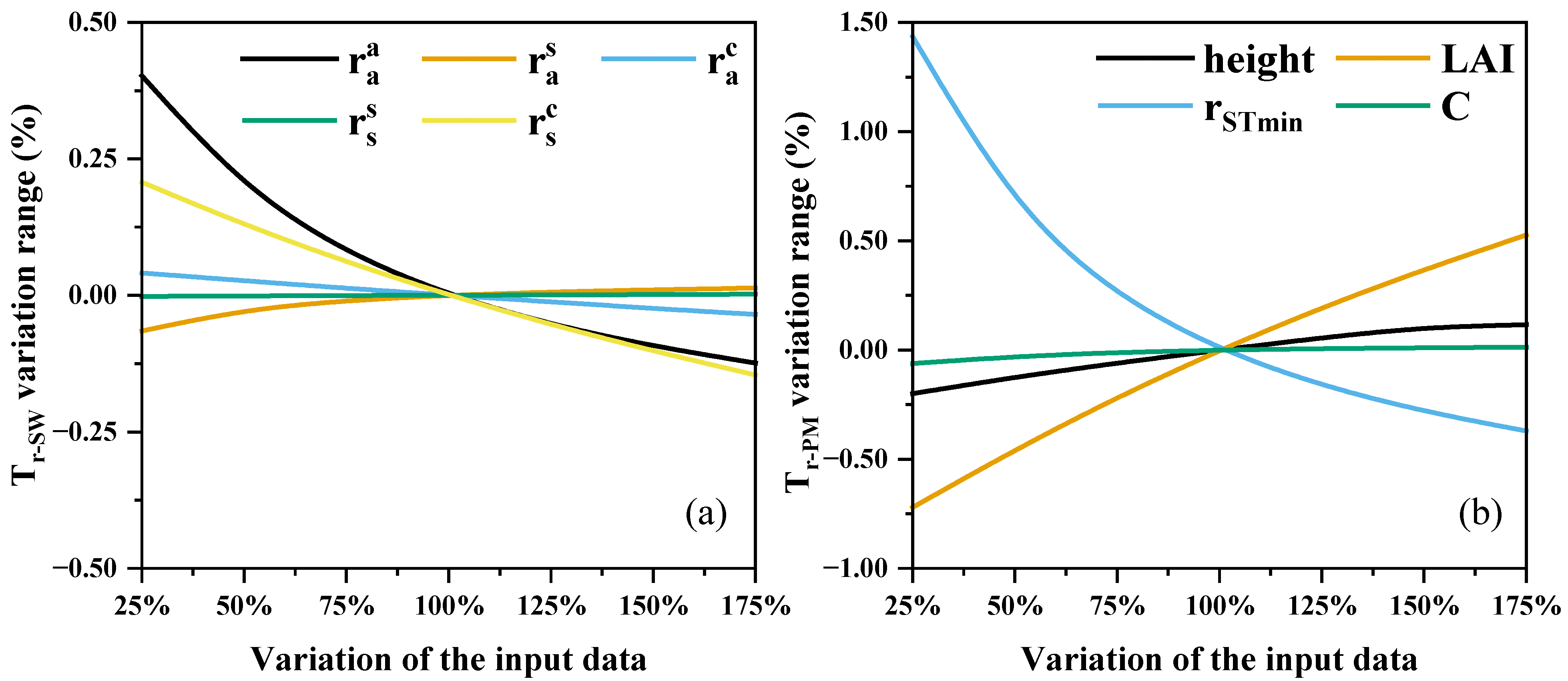
The performance of the PM and SW models greatly depended on the parameters’ situation. We qualified the effects of the parameters’ variation on the estimated transpiration, and the base values of input parameters were from the average values from 16–30 November 2018. The results are summarized in Figure 9. For the PM model, the minimum stomatal resistance rSTmin and LAI had the greatest influence on plant transpiration estimation. When rSTmin and LAI varied by ±25%, the transpiration simulation values ranged from −16.42% to 24.40% and from −21.63% to 19.41%, respectively. The variation of plant height (hc) and extinction coefficient (C) varied by ±25% and had little effect on the transpiration estimation, and the change range was less than 6%. Therefore, the LAI value should be carefully measured. The rSTmin mainly depended on the climatic condition and available soil water. In this study, we used the value of 33.5 s m−1, and the results showed good results for transpiration estimation (Figure 3 and Figure 6). This meant that this value could be used for tomato transpiration estimation by the PM model under sufficient water conditions in the greenhouse.
For the SW model, the estimated transpiration generally increased with the increasing r a s and   r s s , and decreased with the increasing r a a , r a c , and r s c . Among the five resistance parameters, r a a and   r s c had the most significant effect on transpiration, while r a c and   r s s had less influence. When r a a and   r s c parameters varied by ±25%, the estimated transpiration varied from −5.4% to 7.7% and from −5.4% to 6.1%, respectively. However, the simulated Tr increased when r a s and   r s s become larger. This was because r a s and   r s s did not directly affect PMc, but would increase the weight coefficient Cc, resulting in a slight increase in transpiration.

6. Conclusions

The following conclusions can be drawn from this study:
(1)
The PM and SW models performed well in estimating the daily transpiration of greenhouse tomatoes. The original PT model, with a coefficient of 1.26, could underestimate tomato daily transpiration by approximately 30%. With a calibrated coefficient, the PT model perfectly estimated the tomato transpiration with an R2 of 0.94 and slope of 0.98.
(2)
The PM and calibrated PT models also did well in hourly transpiration estimation with an error of 3% and 8%, respectively; however, the SW model underestimated the hourly transpiration by approximately 17%. The SF lag time should be considered when it is used for transpiration analysis.
(3)
The PT model resulted in a large error when plants suffered from heat and water stress, while the PM and SW models performed well in this stressful situation because these situations were considered in the models’ parameters.
(4)
All three models could be used to estimate tomato transpiration in the SSG. The calibrated PT model is strongly recommended because it uses fewer parameters and a simple expression.

Author Contributions

Conception and design of experiments: H.L.; performance of experiments and analysis of data: M.S. and L.Y.; writing—review and editing: M.S. and H.L. All authors have read and agreed to the published version of the manuscript.

Funding

This work was supported by the Ningbo Science and Technology Project (NO. 2022S097), the National Nature Science Foundation of China (NO. 51939005, 91479004) and the 111 Project (B18006).

Institutional Review Board Statement

Not applicable.

Informed Consent Statement

Not applicable.

Data Availability Statement

Data is available when readers are asking for it.

Acknowledgments

We greatly appreciate the cooperation of Jiaqi Wang, the owner of the solar greenhouse and Wenen Ju for helping us prepare the references and data.

Conflicts of Interest

The authors declare no conflict of interest.

References

  1. Badji, A.; Benseddik, A.; Bensaha, H.; Boukhelifa, A.; Hasrane, I. Design, technology, and management of greenhouse: A review. J. Clean. Prod. 2022, 373, 133753. [Google Scholar] [CrossRef]
  2. China Statistical Publishing House. China Statistical Yearbook; China Statistical Publishing House: Beijing, China, 2021. [Google Scholar]
  3. Yang, L.; Liu, H.; Cohen, S.; Gao, Z. Microclimate and Plant Transpiration of Tomato (Solanum lycopersicum L.) in a Sunken Solar Greenhouse in North China. Agriculture 2022, 12, 260. [Google Scholar] [CrossRef]
  4. Liu, H.; Yin, C.; Hu, X.; Tanny, J.; Tang, X. Microclimate Characteristics and Evapotranspiration Estimates of Cucumber Plants in a Newly Developed Sunken Solar Greenhouse. Water 2020, 12, 2275. [Google Scholar] [CrossRef]
  5. Ministry of Water Resources of the People’s Republic of China. China Water Resources Bulletin; China WaterPower Press: Beijing, China, 2021.
  6. Liang, H.; Lv, H.; Batchelor, W.D.; Lian, X.; Wang, Z.; Lin, S.; Hu, K. Simulating nitrate and DON leaching to optimize water and N management practices for greenhouse vegetable production systems. Agric. Water Manag. 2020, 241, 106377. [Google Scholar] [CrossRef]
  7. Sun, Y.; Hu, K.; Fan, Z.; Wei, Y.; Lin, S.; Wang, J. Simulating the fate of nitrogen and optimizing water and nitrogen management of greenhouse tomato in North China using the EU-Rotate_N model. Agric. Water Manag. 2013, 128, 72–84. [Google Scholar] [CrossRef]
  8. Liu, H.; Yuan, B.; Hu, X.; Yin, C. Drip irrigation enhances water use efficiency without losses in cucumber yield and economic benefits in greenhouses in North China. Irrig. Sci. 2021, 40, 135–149. [Google Scholar] [CrossRef]
  9. Du, Y.-D.; Cao, H.-X.; Liu, S.-Q.; Gu, X.-B.; Cao, Y.-X. Response of yield, quality, water and nitrogen use efficiency of tomato to different levels of water and nitrogen under drip irrigation in Northwestern China. J. Integr. Agric. 2017, 16, 1153–1161. [Google Scholar] [CrossRef] [Green Version]
  10. Liang, H.; Hu, K.; Batchelor, W.D.; Qin, W.; Li, B. Developing a water and nitrogen management model for greenhouse vegetable production in China: Sensitivity analysis and evaluation. Ecol. Model. 2018, 367, 24–33. [Google Scholar] [CrossRef]
  11. Liu, H.; Li, H.; Ning, H.; Zhang, X.; Li, S.; Pang, J.; Wang, G.; Sun, J. Optimizing irrigation frequency and amount to balance yield, fruit quality and water use efficiency of greenhouse tomato. Agric. Water Manag. 2019, 226, 105787. [Google Scholar] [CrossRef]
  12. Li, H.; Liu, H.; Gong, X.; Li, S.; Pang, J.; Chen, Z.; Sun, J. Optimizing irrigation and nitrogen management strategy to trade off yield, crop water productivity, nitrogen use efficiency and fruit quality of greenhouse grown tomato. Agric. Water Manag. 2021, 245, 106570. [Google Scholar] [CrossRef]
  13. Shock, C.; Wang, F.-X. Soil Water Tension, a Powerful Tool for Productivity and Stewardship. Am. Soc. Hortic. Sci. 2010, 46, 178–185. [Google Scholar]
  14. Kang, S.Z.; Liu, X.M.; Xiong, Y.Z. Theory of Water Transport in Soil-Plant-Atmosphere Continuum and Its Application; China Water Resources and Hydro-Power Press: Beijing, China, 1994. [Google Scholar]
  15. Evapotranspiration Basics and Estimating Actual Crop Evapotranspiration from Reference Evapotranspiration and Crop-Specific Coefficients. Available online: https://extensionpublications.unl.edu/assets/html/g1994/build/g1994.htm (accessed on 21 September 2022).
  16. Kang, S.; Gu, B.; Du, T.; Zhang, J. Crop coefficient and ratio of transpiration to evapotranspiration of winter wheat and maize in a semi-humid region. Agric. Water Manag. 2003, 59, 239–254. [Google Scholar] [CrossRef]
  17. Allan, R.; Pereira, L.; Smith, M. Crop Evapotranspiration-Guidelines for Computing Crop Water Requirements-FAO Irrigation and Drainage Paper 56; Food and Agriculture Organization of the United Nations (FAO): Rome, Italy, 1998. [Google Scholar]
  18. Montoro, A.; Torija, I.; Mañas, F.; López-Urrea, R. Lysimeter measurements of nocturnal and diurnal grapevine transpiration: Effect of soil water content, and phenology. Agric. Water Manag. 2020, 229, 105882. [Google Scholar] [CrossRef]
  19. Tfwala, C.M.; van Rensburg, L.D.; Bello, Z.A.; Green, S.R. Calibration of compensation heat pulse velocity technique for measuring transpiration of selected indigenous trees using weighing lysimeters. Agric. Water Manag. 2018, 200, 27–33. [Google Scholar] [CrossRef]
  20. Beslity, J.; Shaw, S.B.; Drake, J.E.; Fridley, J.; Stella, J.C.; Stark, J.; Singh, K. A low cost, low power sap flux device for distributed and intensive monitoring of tree transpiration. HardwareX 2022, 12, e00351. [Google Scholar] [CrossRef]
  21. Dix, M.J.; Aubrey, D.P. Calibration approach and range of observed sap flow influences transpiration estimates from thermal dissipation sensors. Agric. For. Meteorol. 2021, 307, 108534. [Google Scholar] [CrossRef]
  22. Zeggaf, A.T.; Takeuchi, S.; Dehghanisanij, H.; Anyoji, H.; Yano, T. A Bowen Ratio Technique for Partitioning Energy Fluxes between Maize Transpiration and Soil Surface Evaporation. Agron. J. 2008, 100, 988–996. [Google Scholar] [CrossRef]
  23. Wang, F.; Ma, D.; Zhao, W.; Lu, Y.; Zhou, D.; Zhang, J.; Chen, L.; Huang, P.; Naeth, M.A. A validation of eddy covariance technique for measuring crop evapotranspiration on different time scales in the North China Plain. Can. J. Soil Sci. 2021, 101, 134–146. [Google Scholar] [CrossRef]
  24. Shuttleworth, W.J.; Wallace, J.S. Evaporation from sparse crops—An energy combination theory. Q. J. R. Meteorol. Soc. 1985, 111, 839–855. [Google Scholar] [CrossRef]
  25. Priestley, C.H.B.; Taylor, R.J. On the Assessment of Surface Heat Flux and Evaporation Using Large-Scale Parameters. Mon. Weather. Rev. 1972, 100, 81–92. [Google Scholar] [CrossRef]
  26. López-Cruz, I.L.; Olivera-López, M.; Herrera-Ruiz, G. Simulation of greenhouse tomato crop transpiration by two theoretical models. International Workshop on Greenhouse Environmental Control and Crop Production in Semi-Arid Regions; International Society for Horticultural Science: Tucson, AZ, USA, 2008; pp. 145–150. [Google Scholar]
  27. Huang, S.; Yan, H.; Zhang, C.; Wang, G.; Acquah, S.J.; Yu, J.; Li, L.; Ma, J.; Opoku Darko, R. Modeling evapotranspiration for cucumber plants based on the Shuttleworth-Wallace model in a Venlo-type greenhouse. Agric. Water Manag. 2020, 228, 105861. [Google Scholar] [CrossRef]
  28. Guo, D.; Chen, Z.; Huang, D.; Zhang, J. Evapotranspiration Model-based Scheduling Strategy for Baby Pakchoi Irrigation in Greenhouse. HortScience 2021, 56, 204–209. [Google Scholar] [CrossRef]
  29. Zheng, S.; Wang, T.; Wei, X. Estimating grapevine transpiration in greenhouse with three different methods in a Penman–Monteith model in Northeast China. Irrig. Sci. 2021, 40, 13–27. [Google Scholar] [CrossRef]
  30. Li, X.; Yang, P.; Ren, S.; Li, Y.; Xu, T.; Ren, L.; Wang, C. An improved canopy transpiration model and parameter uncertainty analysis by Bayesian approach. Math. Comput. Model. 2010, 51, 1368–1374. [Google Scholar] [CrossRef]
  31. Gong, X.; Liu, H.; Sun, J.; Gao, Y.; Zhang, X.; Jha, S.K.; Zhang, H.; Ma, X.; Wang, W. A proposed surface resistance model for the Penman-Monteith formula to estimate evapotranspiration in a solar greenhouse. J. Arid. Land 2017, 9, 530–546. [Google Scholar] [CrossRef]
  32. Yan, H.; Acquah, S.J.; Zhang, C.; Wang, G.; Huang, S.; Zhang, H.; Zhao, B.; Wu, H. Energy partitioning of greenhouse cucumber based on the application of Penman-Monteith and Bulk Transfer models. Agric. Water Manag. 2019, 217, 201–211. [Google Scholar] [CrossRef]
  33. Brisson, N.; Itier, B.; L’Hotel, J.C.; Lorendeau, J.Y. Parameterisation of the Shuttleworth-Wallace model to estimate daily maximum transpiration for use in crop models. Ecol. Model. 1998, 107, 159–169. [Google Scholar] [CrossRef]
  34. Zhang, B.; Kang, S.; Zhang, L.; Tong, L.; Du, T.; Li, F.; Zhang, J. An evapotranspiration model for sparsely vegetated canopies under partial root-zone irrigation. Agric. For. Meteorol. 2009, 149, 2007–2011. [Google Scholar] [CrossRef]
  35. Li, S.; Kang, S.; Zhang, L.; Ortega-Farias, S.; Li, F.; Du, T.; Tong, L.; Wang, S.; Ingman, M.; Guo, W. Measuring and modeling maize evapotranspiration under plastic film-mulching condition. J. Hydrol. 2013, 503, 153–168. [Google Scholar] [CrossRef]
  36. Assouline, S.; Li, D.; Tyler, S.; Tanny, J.; Cohen, S.; Bou-Zeid, E.; Parlange, M.; Katul, G.G. On the variability of the Priestley-Taylor coefficient over water bodies. Water Resour. Res. 2016, 52, 150–163. [Google Scholar] [CrossRef] [Green Version]
  37. Engstrom, R.; Hope, A.; Stow, D.; Vourlitis, G.; Oechel, W. Priestley-Taylor Alpha Coefficient: Variability and Relationship to NDVI in Arctic Tundra Landscapes. J. Am. Water Resour. Assoc. 2007, 38, 1647–1659. [Google Scholar] [CrossRef]
  38. Qiu, R.; Liu, C.; Cui, N.; Wu, Y.; Wang, Z.; Li, G. Evapotranspiration estimation using a modified Priestley-Taylor model in a rice-wheat rotation system. Agric. Water Manag. 2019, 224, 105755. [Google Scholar] [CrossRef]
  39. Valdés-Gómez, H.; Ortega-Farías, S.; Argote, M. Evaluation of the Water Requirements for a Greenhouse Tomato Crop using the Priestley-Taylor Method Evaluación del Consumo de Agua de un Cultivo de Tomate en Invernadero Usando el Método de Priestley-Taylor. Chil. J. Agric. Res. 2009, 69, 3–11. [Google Scholar] [CrossRef] [Green Version]
  40. Thom, A.; Oliver, H. On Penman’s Equation for Estimating Regional Evaporation. Q. J. R. Meteorol. Soc. 2006, 103, 345–357. [Google Scholar] [CrossRef]
  41. Gong, X.W.; Ge, J.K.; Li, Y.B.; Wang, S.S.; Zhang, H.; Zhang, L.; Liu, Y.F.; Liu, H. Evaluation of the dual source model to simulate transpiration and evaporation of tomato plants cultivated in a solar greenhouse. Eur. J. Hortic. Sci. 2020, 85, 362–371. [Google Scholar] [CrossRef]
  42. Nikolaou, G.; Neocleous, D.; Kitta, E.; Katsoulas, N. Assessment of the Priestley-Taylor coefficient and a modified potential evapotranspiration model. Smart Agric. Technol. 2023, 3, 100075. [Google Scholar] [CrossRef]
  43. Gong, X.; Qiu, R.; Ge, J.; Bo, G.; Ping, Y.; Xin, Q.; Wang, S. Evapotranspiration partitioning of greenhouse grown tomato using a modified Priestley–Taylor model. Agric. Water Manag. 2021, 247, 106709. [Google Scholar] [CrossRef]
  44. Zhou, M.C.; Ishidaira, H.; Hapuarachchi, H.P.; Magome, J.; Kiem, A.S.; Takeuchi, K. Estimating potential evapotranspiration using Shuttleworth–Wallace model and NOAA-AVHRR NDVI data to feed a distributed hydrological model over the Mekong River basin. J. Hydrol. 2006, 327, 151–173. [Google Scholar] [CrossRef]
  45. Moriasi, D.N.; Arnold, J.G.; Van Liew, M.W.; Bingner, R.L.; Harmel, R.D.; Veith, T.L. Model evaluation guidelines for systematic quantification of accuracy in watershed simulations. Trans. ASABE 2007, 50, 885–900. [Google Scholar] [CrossRef]
  46. Li, Y.; Xue, X.; Guo, W.; Wang, L.; Duan, M.; Chen, H.; Chen, F. Soil moisture and nitrate-nitrogen dynamics and economic yield in the greenhouse cultivation of tomato and cucumber under negative pressure irrigation in the North China Plain. Sci. Rep. 2019, 9, 4439. [Google Scholar]
  47. CAO, D. Effects of Alternative Root-Splitting Irrigation on Tomato Growth and Water Distribution; Heibei Agricultrual University: Hebei, China, 2020. [Google Scholar]
  48. Gong, X.; Wang, S.; Xu, C.; Zhang, H.; Ge, J. Evaluation of Several Reference Evapotranspiration Models and Determination of Crop Water Requirement for Tomato in a Solar Greenhouse. HortScience 2020, 55, 244–250. [Google Scholar] [CrossRef] [Green Version]
  49. Ghiat, I.; Mackey, H.R.; Al-Ansari, T. A Review of Evapotranspiration Measurement Models, Techniques and Methods for Open and Closed Agricultural Field Applications. Water 2021, 13, 2523. [Google Scholar] [CrossRef]
  50. Wang, L.; Iddio, E.; Ewers, B. Introductory overview: Evapotranspiration (ET) models for controlled environment agriculture (CEA). Comput. Electron. Agric. 2021, 190, 106447. [Google Scholar] [CrossRef]
  51. Katsoulas, N.; Stanghellini, C. Modelling Crop Transpiration in Greenhouses: Different Models for Different Applications. Agronomy 2019, 9, 392. [Google Scholar] [CrossRef] [Green Version]
  52. Villarreal-Guerrero, F.; Kacira, M.; Fitz-Rodríguez, E.; Linker, R.; Kubota, C.; Giacomelli, G.A.; Arbel, A. Simulated performance of a greenhouse cooling control strategy with natural ventilation and fog cooling. Biosyst. Eng. 2012, 111, 217–228. [Google Scholar] [CrossRef]
  53. Hobbins, M.T.; Ramírez, J.A.; Brown, T.C. The complementary relationship in estimation of regional evapotranspiration: An enhanced advection-aridity model. Water Resour. Res. 2001, 37, 1389–1403. [Google Scholar] [CrossRef] [Green Version]
  54. De Bruin, H.A.R. A Model for the Priestley-Taylor Parameter α. J. Clim. Appl. Meteorol. 1983, 22, 572–578. [Google Scholar] [CrossRef]
  55. Juhász, Á.; Hrotkó, K. Comparison of the transpiration part of two sources evapotranspiration model and the measurements of sap flow in the estimation of the transpiration of sweet cherry orchards. Agric. Water Manag. 2014, 143, 142–150. [Google Scholar] [CrossRef]
  56. Gong, X.; Liu, H.; Sun, J.; Gao, Y.; Zhang, H. Comparison of Shuttleworth-Wallace model and dual crop coefficient method for estimating evapotranspiration of tomato cultivated in a solar greenhouse. Agric. Water Manag. 2019, 217, 141–153. [Google Scholar] [CrossRef]
  57. Chen, Y.J.; Bongers, F.; Tomlinson, K.; Fan, Z.X.; Lin, H.; Zhang, S.B.; Zheng, Y.L.; Li, Y.P.; Cao, K.F.; Zhang, J.L. Time lags between crown and basal sap flows in tropical lianas and co-occurring trees. Tree Physiol. 2016, 36, 736–747. [Google Scholar] [CrossRef] [Green Version]
  58. Liu, H.-J.; Cohen, S.; Tanny, J.; Lemcoff, J.H.; Huang, G. Transpiration estimation of banana (Musa sp.) plants with the thermal dissipation method. Plant Soil 2008, 308, 227–238. [Google Scholar] [CrossRef]
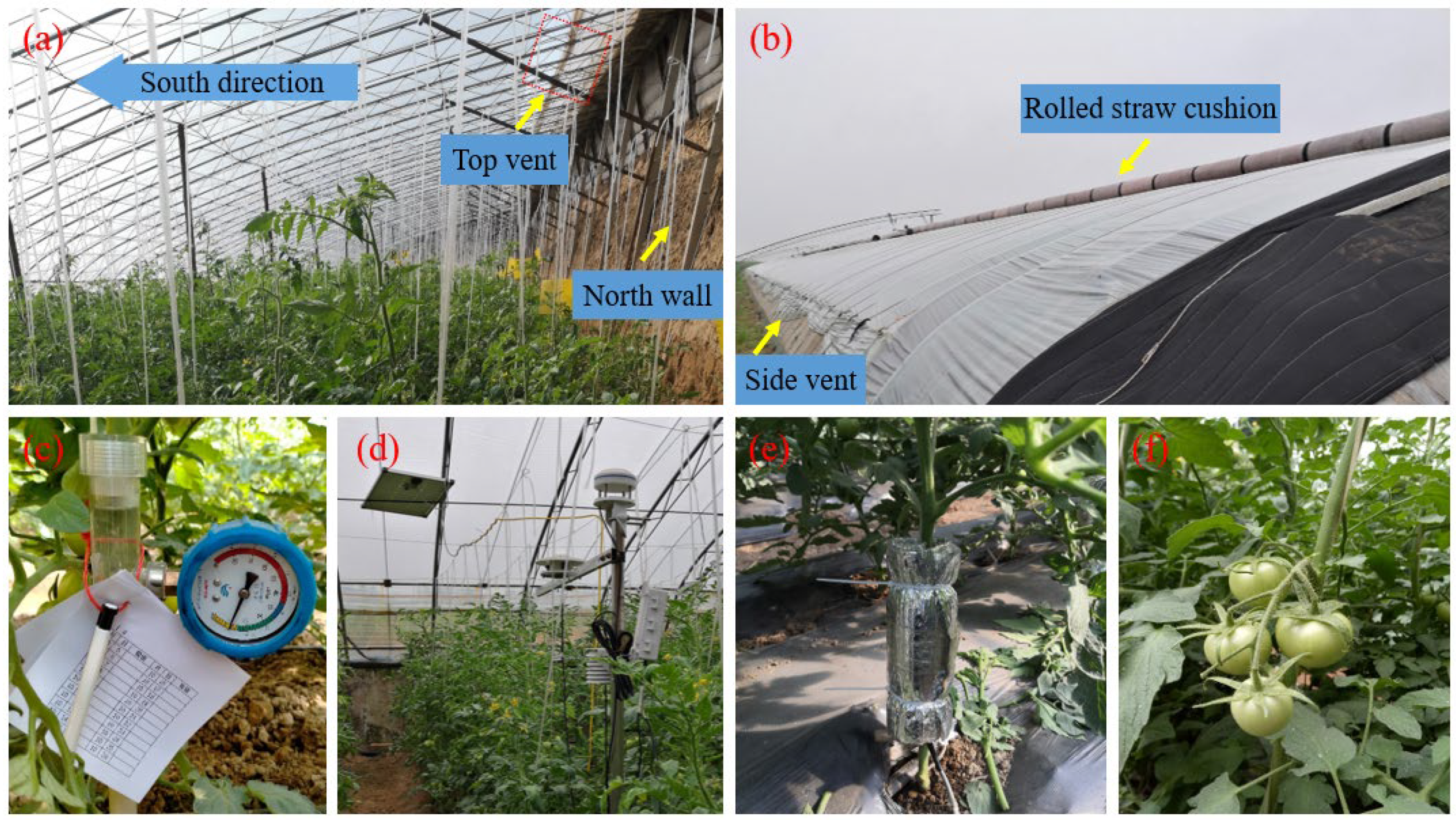
Figure 1. Photos of the sunken solar greenhouse. (a) inside view with tomato growth, (b) outside view in winter, with front plastic cover facing south and the rolled straw cushion placed on the top of the roof, (c) soil matric measurement using dial type tensiometer, (d) a view of the meteorological station, (e) a view of one set of sap flow gauge, and (f) a view of the growing tomato.
Agronomy 12 02382 g001
Figure 2. Variations of daily mean micrometeorological elements in the sunken solar greenhouse during the 2018–2020 winter periods. (a) daily maximum (Tmax), minimum (Tmin), and mean air temperature (Ta), (b) net radiation (Rn), and (c) relative humidity (RH) and vapor pressure deficit (VPD).
Agronomy 12 02382 g002
Figure 3. Comparison of the simulated daily crop transpiration by PM (Tr-PM, a), SW (Tr-SW, b), and PT (Tr-PT, c) Methods and measured sap flow (SF) during the three winter seasons. In (c), lines of PT indicated that the daily Tr was estimated using the original PT model with α of 1.26, and that in PT(αm) the line was estimated using α regulated by Equation (28).
Agronomy 12 02382 g003
Figure 4. Correlation between daily simulated values and the measured sap flow (SF) for winter of 2018 (a), 2019 (b), 2020(c), and for all three winters (d).
Agronomy 12 02382 g004
Figure 5. Correlation between simulated daily transpiration (Tr-PT) by the PT model using the original coefficient α of 1.26 (PT(α = 1.26)) and the calibrated α using Equation (28) and the measured daily sap flow (SF) during the three winter seasons.
Agronomy 12 02382 g005
Figure 6. Daily courses of the simulated hourly Tr values by the PM (a), SW (b) and calibrated PT (c) models and the measured sap flow (SF) during the seven sample days from 4–10 November in the 2019 winter season.
Agronomy 12 02382 g006
Figure 7. Daily courses of hourly air temperature (a), net radiation (b), vapor pressure deficit (c), and relative humidity (d) in the sunken solar greenhouse from 4 to 10 November in the 2019 season.
Agronomy 12 02382 g007
Figure 8. Correlation between simulated hourly Tr and the measured sap flow (SF) when the SF lag time was not considered (a) and considered (b) during the seven sample days in the 2019 winter season.
Agronomy 12 02382 g008
Figure 9. Sensitivity Analysis of SW (a) and PM (b) Models.
Agronomy 12 02382 g009
Table 1. Fertilization amounts for three winter seasons.
Planting SeasonsFertilizationN
kg ha−1
P2O5
kg ha−1
K2O
kg ha−1
2018 winterbase fertilization114114114
topdressing fertilization6823159
total182137273
2019 winterbase fertilization114114114
topdressing fertilization919191
total205205205
2020 winterbase fertilization171171171
topdressing fertilization919191
total262262262
Table 2. Irrigation amount and irrigation events for three winter seasons.
Planting SeasonsTotal Irrigation Depth (mm) *Sap Flow Measurement Period **
Irrigation Depth
(mm)
Irrigation EventsIrrigation Depth Per Time (mm)
2018 winter516255642.5
2019 winter508162627.0
2020 winter461250550.0
Note: * Total irrigation depth is the total amount of irrigation during the whole growth period in each winter season. ** The data in the columns for irrigation depth, irrigation events, and irrigation depth per time were only recorded in the sap flow measurement period.
Table 3. General performance ratings [45].
NSERSRPerformance Rating
0.75 < NSE ≤ 10 ≤ RSR ≤ 0.5Very good
0.65 < NSE < 0.750.5 < RSR < 0.6Good
0.5 < NSE < 0.650.6 < RSR < 0.7Satisfactory
NSE ≤ 0.5RSR > 0.7Unsatisfactory
Table 4. Daily meteorological conditions and tomato plant parameters for selected periods.
Date
2019
RHmean
%
Tmax
°C
Ta
°C
u
m s−1
VPD
kPa
Rn
MJ m−2 d−1
LAI
-
h
m
4 Nov81.6228.9018.320.290.504.651.601.21
5 Nov83.4231.4019.250.220.504.391.601.21
6 Nov86.8828.8018.400.200.363.431.591.21
7 Nov91.9623.9016.960.270.182.471.591.21
8 Nov87.7231.2018.330.320.363.891.591.21
9 Nov91.0926.5017.940.250.222.831.591.22
10 Nov82.0642.2021.210.310.894.941.581.22
Publisher’s Note: MDPI stays neutral with regard to jurisdictional claims in published maps and institutional affiliations.