Appendix A
Table A1.
Updated fields in production inventories.
Table A1.
Updated fields in production inventories.
| Field | Task | Auxiliary Information |
|---|
| feed | estimate missing information | average Milk production, feedbase, SALCA model farms |
| climate data | estimate missing information | Swiss Meteo monthly averages |
| fertilizer application date | estimate missing information | “Feldkalender AUI” |
| plant protection | correction | Swiss Register of plant protection products |
| Nitrogen in farmyard manure | estimate missing information | GRUD “Grundlagen für die Düngung landwirtschaftlicher Kulturen in der Schweiz” |
| straw application | estimate missing information | SALCA model farms |
| GVE coefficients | estimate missing information | “Faktoren für die Umrechnung des Tierbestandes in Grossvieheinheiten” |
| fresh substance to dry matter coefficients | estimate missing information | SALCA internal data |
| farmyard manure systems | estimate missing information | SALCA model farms |
| period on pasture | estimate missing information | SALCA model farms |
| occupation | estimate missing information | SALCA internal data |
| time spent in yard | estimate missing information | SALCA model farms |
| time spent on pasture | estimate missing information | SALCA model farms |
| fertilizer composition | estimate missing information | SALCA internal data |
| crop codes | estimate missing information | SALCA internal data |
Table A2.
Overview of all defined product groups. The column “Included in study” indicates if the product group was considered important and homogenous enough to be included in this study. N denotes the total available observations.
Table A2.
Overview of all defined product groups. The column “Included in study” indicates if the product group was considered important and homogenous enough to be included in this study. N denotes the total available observations.
| Field | Task | Auxiliary Information |
|---|
| Cattle | 240 | TRUE |
| Milk | 180 | TRUE |
| Cereals | 173 | TRUE |
| Remaining feed/arable crops | 139 | FALSE |
| Remaining animals | 107 | FALSE |
| Fruits | 55 | TRUE |
| Pig fattening | 47 | TRUE |
| Potatoes | 44 | TRUE |
| Beets | 40 | TRUE |
| Vegetables | 38 | TRUE |
| Corn | 19 | FALSE |
| Non-food | 15 | FALSE |
| Viticulture | 15 | FALSE |
| Pig breeding | 10 | FALSE |
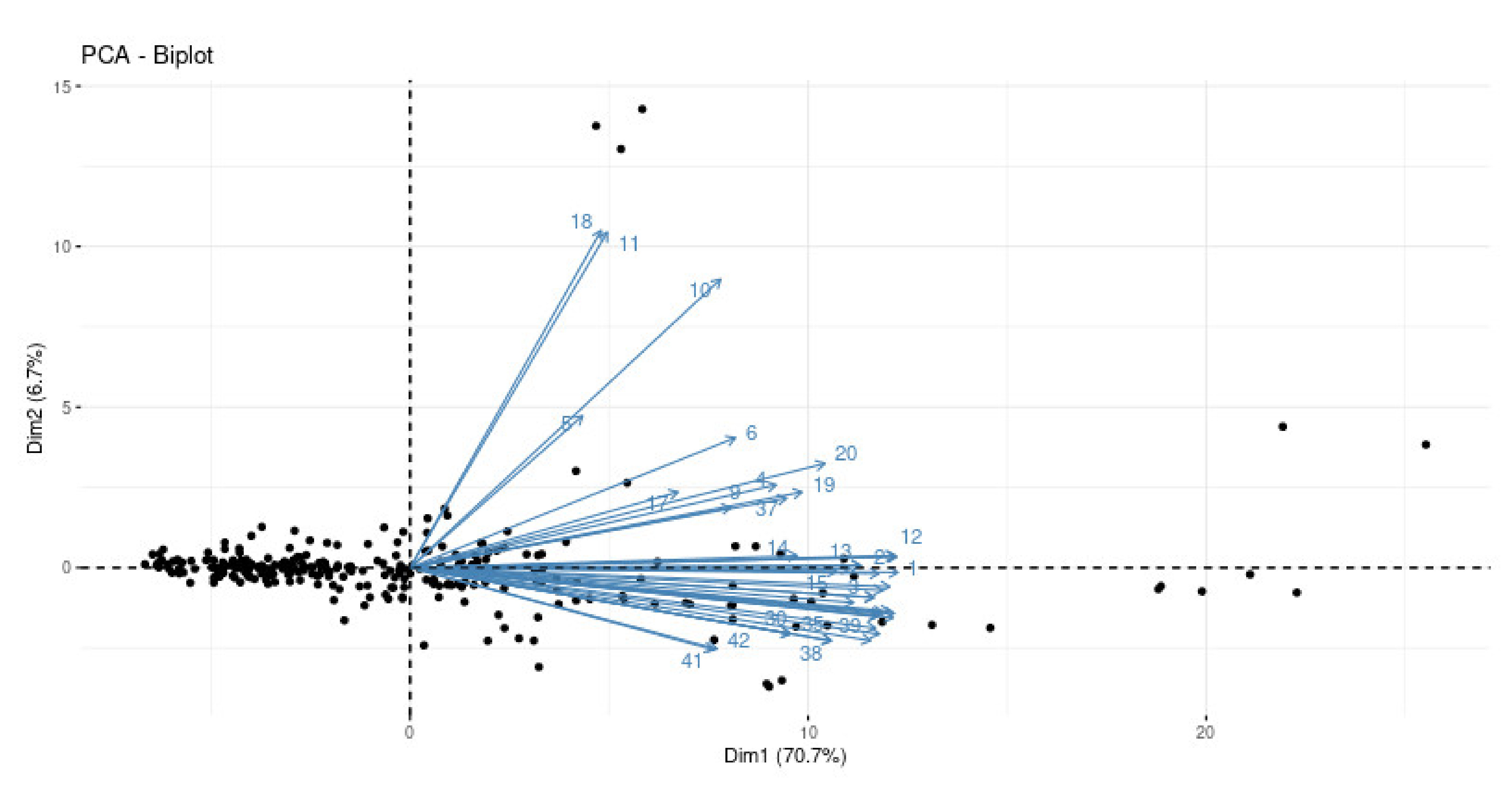
Figure A1.
Principal component analysis of environmental impacts: Two main components explain 77.4% of the total variance. 1 = Non renewable fossil and nuclear (MJ eq), 2 = Non renewable fossil (MJ eq), 3 = Non renewable nuclear (MJ eq), 4 = Resources abiotic (kg of Antimony eq), 5 = Resources potassium K (kg), 6 = Resources phosphorus P (kg), 7 = Land competition (m2a), 8 = Human digestible protein production potential (kg), 9 = Deforestation (m2), 10 = Total water use blue water (m3), 11 = Water Stress Index (m3), 12 = Exergy non renewable fossil (MJ), 13 = Exergy non renewable nuclear (MJ), 14 = Exergy renewable wind (MJ), 15 = Exergy renewable solar (MJ), 16 = Exergy renewable hydro (MJ), 17 = Exergy non renewable primary forest (MJ), 18 = Exergy renewable water (MJ), 19 = Exergy non renewable metals (MJ), 20 = Exergy non renewable minerals (MJ), 21 = Exergy land resources (MJ), 22 = Exergy total (MJ), 23 = IPCC GWP 100a 2013 (kg CO2 eq), 24 = IPCC GWP 20a 2013 (kg CO2 eq), 25 = Ozone depletion (kg Trichlorfluormethan eq), 26 = Photochemical ozone formation (kg Non Methane Volatile Organic Compounds eq), 27 = Acidification GLO (molc H+ eq), 28 = Eutrophication terr. GLO (m2), 29 = Eutrophication aq. N GLO (kg N), 30 = Eutrophication aq. P GLO (kg P), 31 = Eutrophication norm. GLO (person year), 32 = Acidification CH (molc H+ eq), 33 = Eutrophication terrestrial CH (m2), 34 = Eutrophication aq. N CH (kg N), 35 = Eutrophication aq. P CH (kg P), 36 = Eutrophication normalized CH (person year), 37 = Freshwater ecotoxicity USEtox org (PAF m3 day), 38 = Freshwater ecotoxicity USEtox inorg (PAF m3 day), 39 = Freshwater ecotoxicity USEtox (PAF m3 day), 40 = Human toxicity USEtox cancer (cases), 41 = Human toxicity USEtox noncancer (cases), 42 = Human toxicity USEtox (cases). (MJ = megajoule, eq = equivalent, GWP = Global warming potential, GLO = Global, CH = Switzerland, aq = aquatic, FWater = Freshwater, PAF m3 day = potentially affected fraction of species integrated over time and volume).
![Agronomy 11 01862 g0a1]()
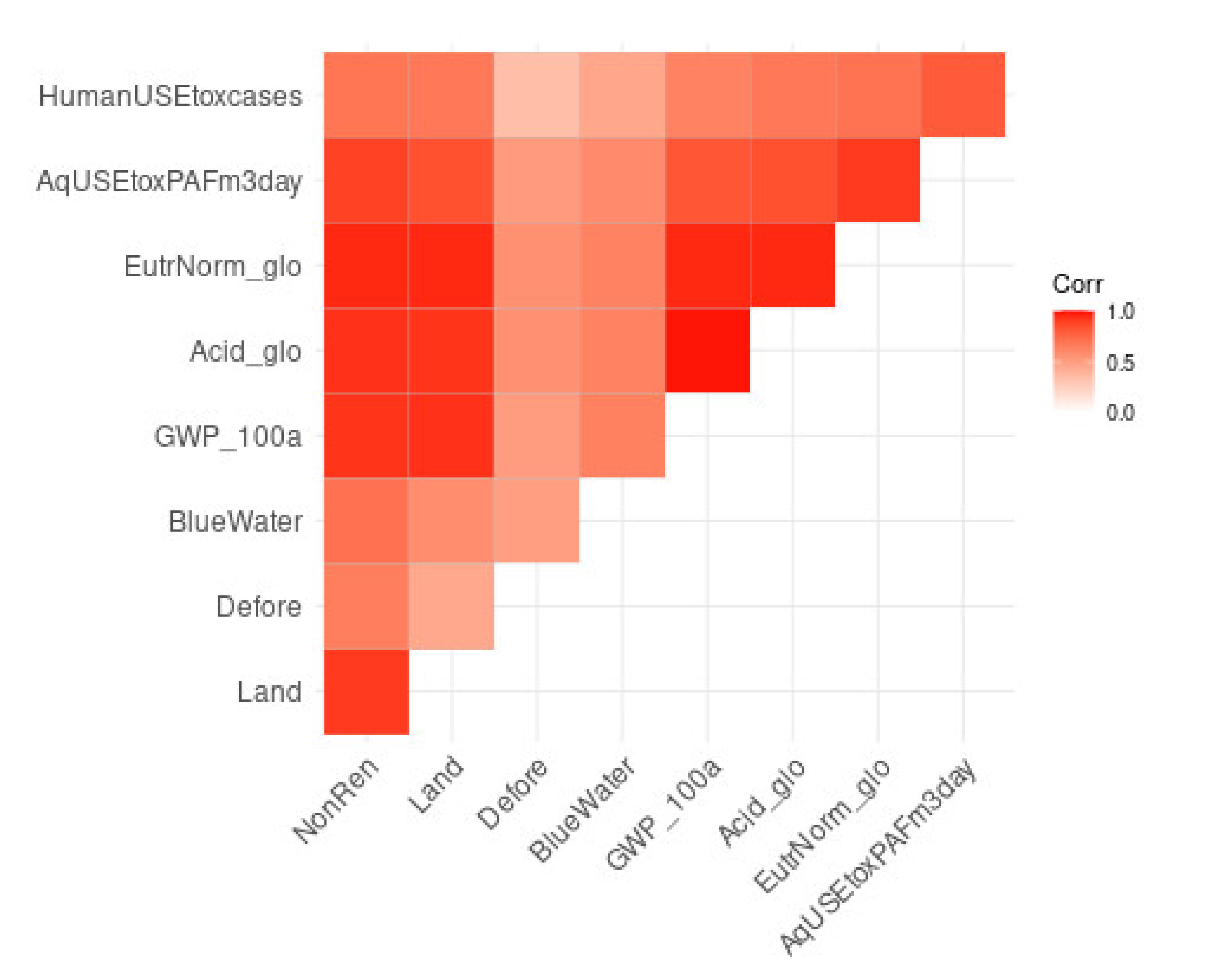
Figure A2.
Correlation coefficients environmental impact indicators (all shown coefficients have p-values < 0.05).
Figure A2.
Correlation coefficients environmental impact indicators (all shown coefficients have p-values < 0.05).
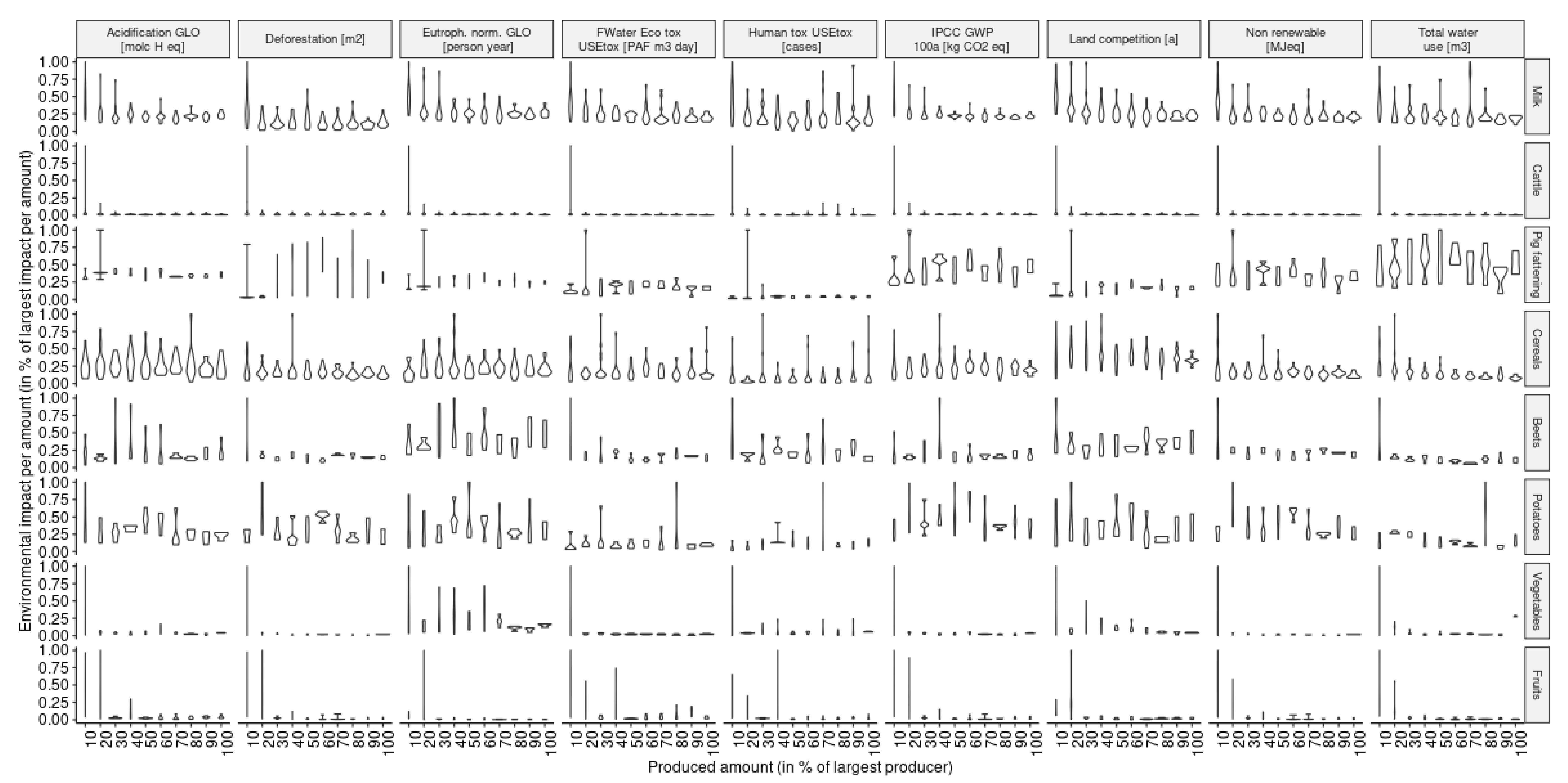
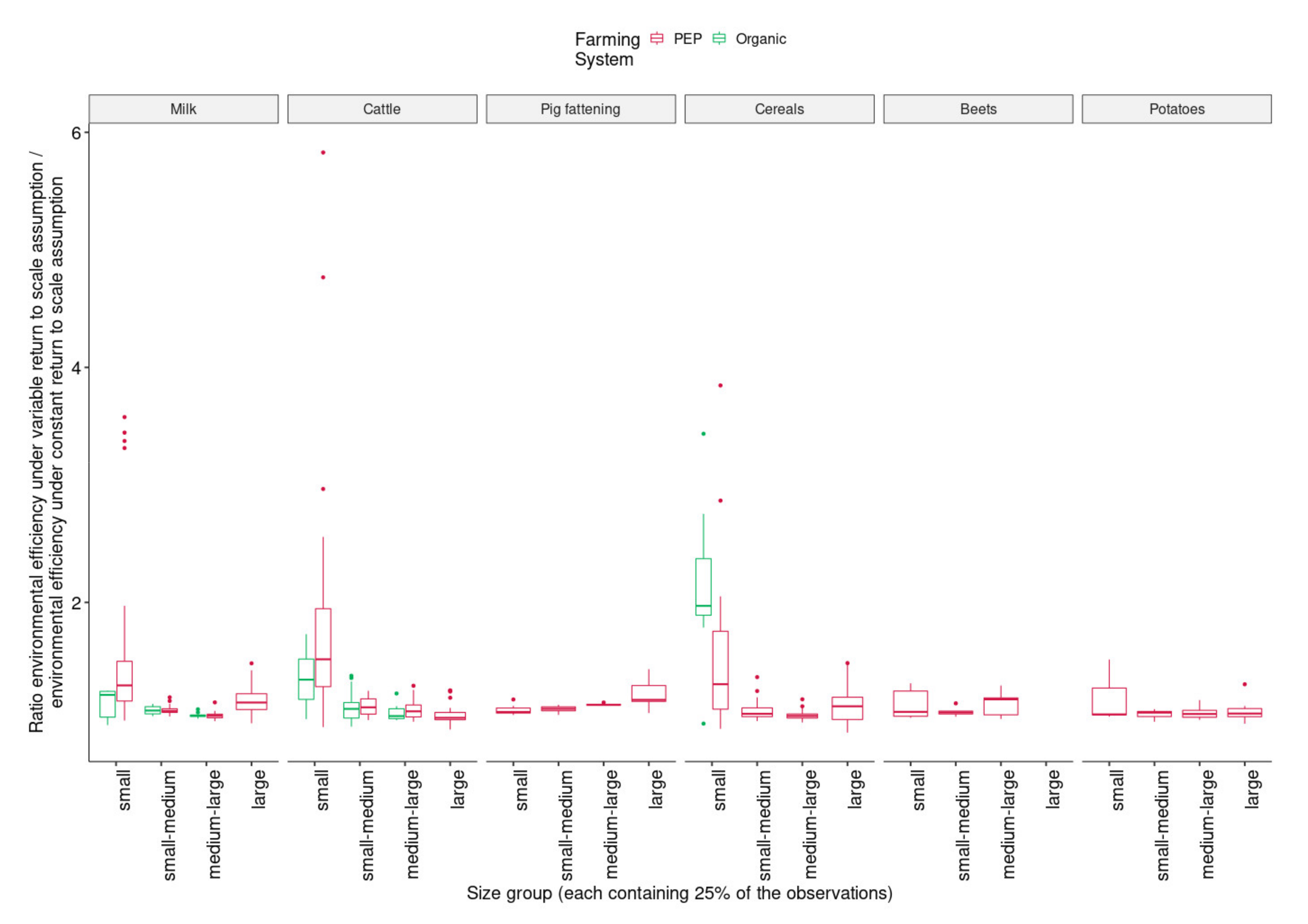
Figure A3.
Variance in environmental efficiency estimate vs. product group size
(measured as output). Smaller product groups show larger variance in estimates. (PAF m3 day = potentially affected fraction of species integrated over time and volume, eq = equivalent, MJ = megajoule).
Figure A3.
Variance in environmental efficiency estimate vs. product group size
(measured as output). Smaller product groups show larger variance in estimates. (PAF m3 day = potentially affected fraction of species integrated over time and volume, eq = equivalent, MJ = megajoule).
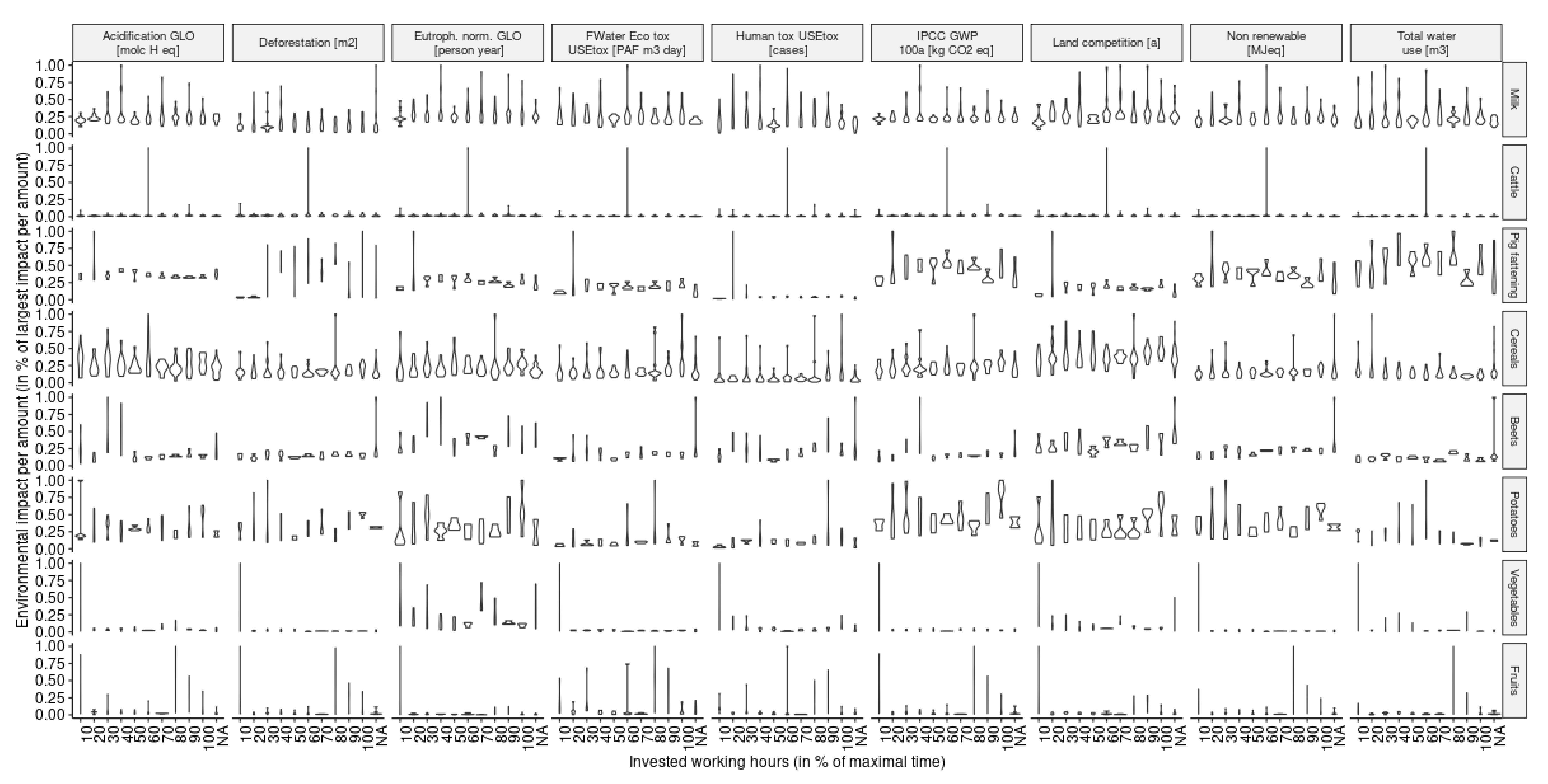
Figure A4.
Variance in environmental efficiency estimate vs. product group size (measured as working hours). Smaller product groups show larger variance in estimates. (PAF m3 day = potentially affected fraction of species integrated over time and volume, eq = equivalent, MJ = megajoul.
Figure A4.
Variance in environmental efficiency estimate vs. product group size (measured as working hours). Smaller product groups show larger variance in estimates. (PAF m3 day = potentially affected fraction of species integrated over time and volume, eq = equivalent, MJ = megajoul.
Table A3.
Amount of product groups by farming system (LW = live weight, DM = dry matter, PEP = Proof of Ecological Performance). Groups with N in parenthesis were not used in the analysis.
Table A3.
Amount of product groups by farming system (LW = live weight, DM = dry matter, PEP = Proof of Ecological Performance). Groups with N in parenthesis were not used in the analysis.
| | Organic | PEP |
|---|
| Product Group | Unit | N | Total | Mean | Median | SD | N | Total | Mean | Median | SD |
|---|
| Milk | Kg | 34 | 3,670,000 | 108,000 | 99,100 | 39,700 | 119 | 15,000,000 | 126,000 | 111,000 | 72,900 |
| Cattle | Kg LW | 31 | 175,000 | 5650 | 5240 | 1960 | 112 | 1,500,000 | 13,400 | 7110 | 21,600 |
| Pig fattening | Kg LW | 4 | 78,100 | 19,500 | 23,500 | 11,700 | 27 | 893,000 | 33,100 | 20,200 | 36,200 |
| Cereals | Kg DM | 12 | 225,000 | 18,800 | 15,200 | 11,500 | 85 | 3,170,000 | 37,300 | 31,600 | 22,600 |
| Beets | Kg DM | | | | | | 19 | 826,000 | 43,500 | 45,400 | 20,000 |
| Potatoes | Kg DM | 4 | 18,900 | 4720 | 1170 | 7390 | 25 | 419,000 | 16,700 | 8340 | 18,500 |
| Vegetables | Kg DM | 6 | 59,800 | 9960 | 9010 | 7440 | 21 | 295,000 | 14,000 | 9700 | 15,800 |
| Fruits | Kg DM | 4 | 5530 | 1380 | 1370 | 358 | 32 | 111,000 | 3470 | 1570 | 4840 |
Table A4.
Human digestible energy content of product groups. DM = Dry Matter, LW = Live Weight.
Table A4.
Human digestible energy content of product groups. DM = Dry Matter, LW = Live Weight.
| Product Group | Units | Energy Content |
|---|
| Milk | (MJ/kg) | 2.8 |
| Fruits | (MJ/kg DM) | 13.4 |
| Cereals | (MJ/kg DM) | 7.3 |
| Cattle | (MJ/kg LW) | 6.1 |
| Pig fattening | (MJ/kg LW) | 14.7 |
| Vegetables | (MJ/kg DM) | 16.5 |
| Beets | (MJ/kg DM) | 12.5 |
| Potatoes | (MJ/kg DM) | 10.5 |
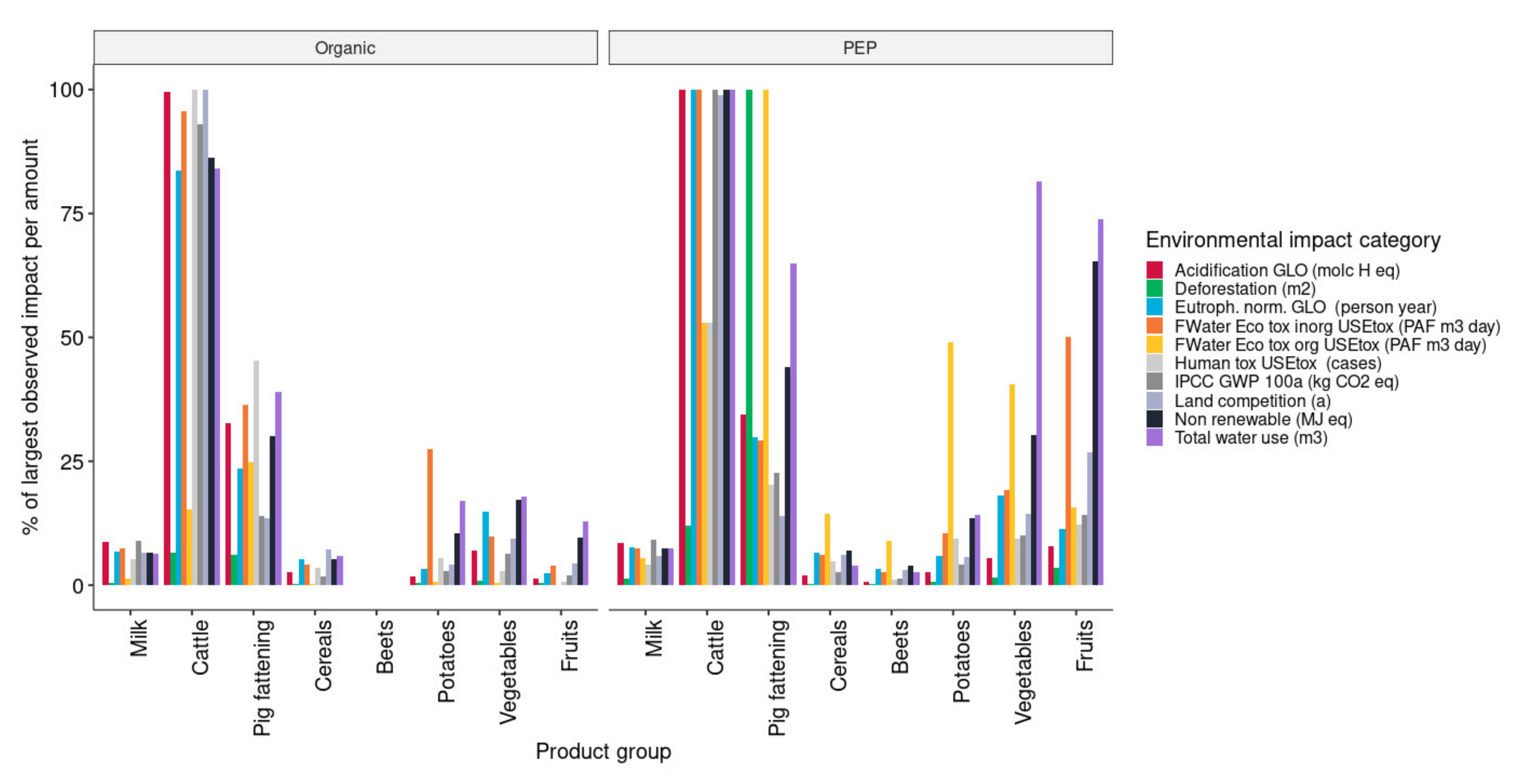
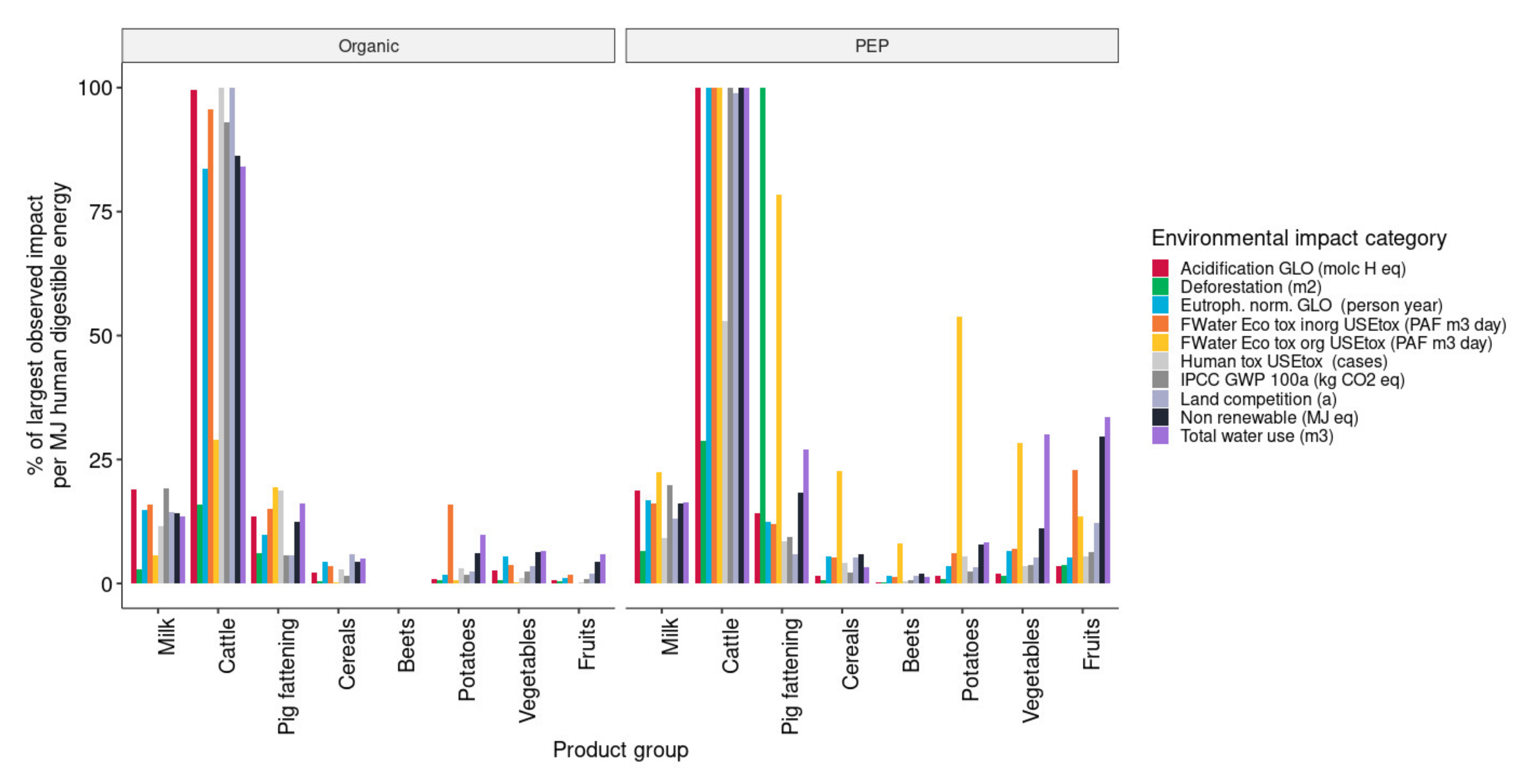
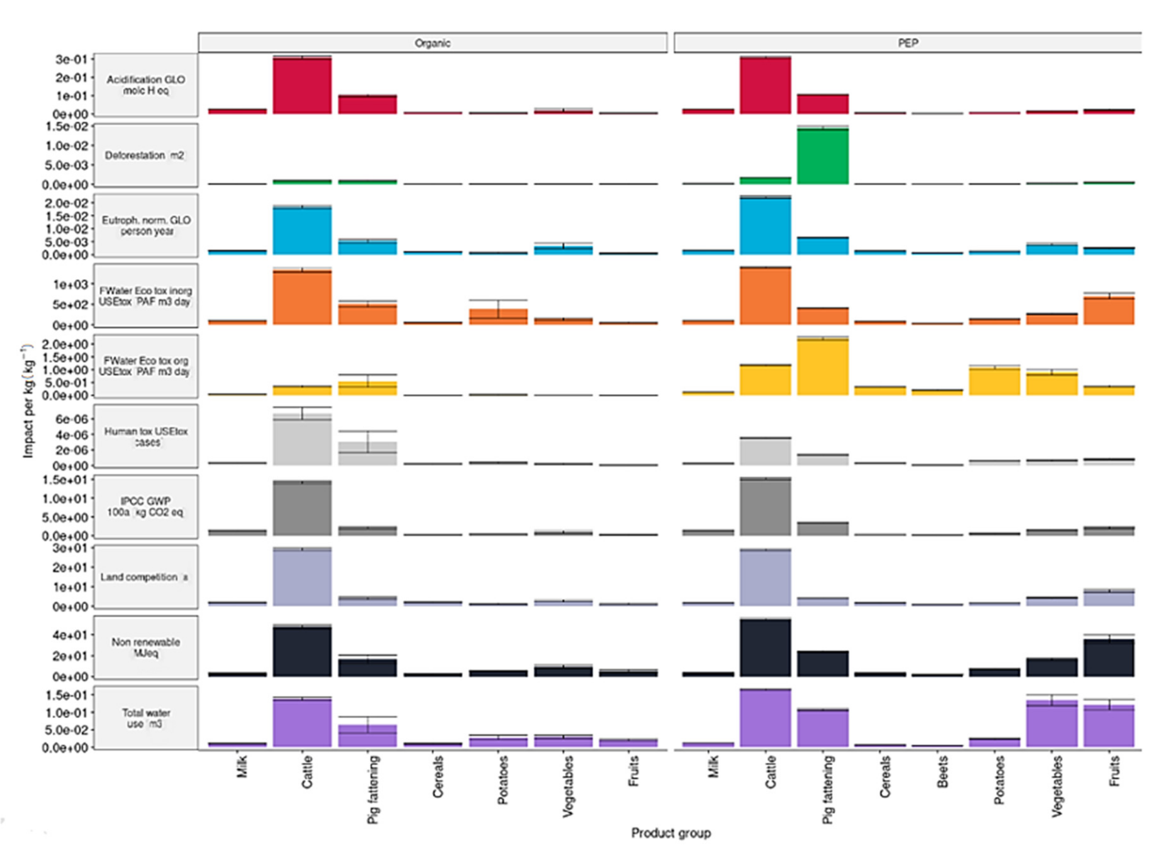
Figure A5.
Environmental impacts per produced amount (kg) for the different product groups and farming systems. Shown are mean values and 95% confidence interval.
Figure A5.
Environmental impacts per produced amount (kg) for the different product groups and farming systems. Shown are mean values and 95% confidence interval.
In order to compare the environmental efficiency of different product groups, we have to define a common functional unit that allows for the comparison of the different products. Here we used the nutritional criteria “human digestible energy content in mega joules [MJ]” (
Appendix A,
Table A4 for conversion factors) as outputs. Accordingly, the resulting environmental efficiency relates the amount of human digestible energy to the environmental impacts. As shown in
Appendix A,
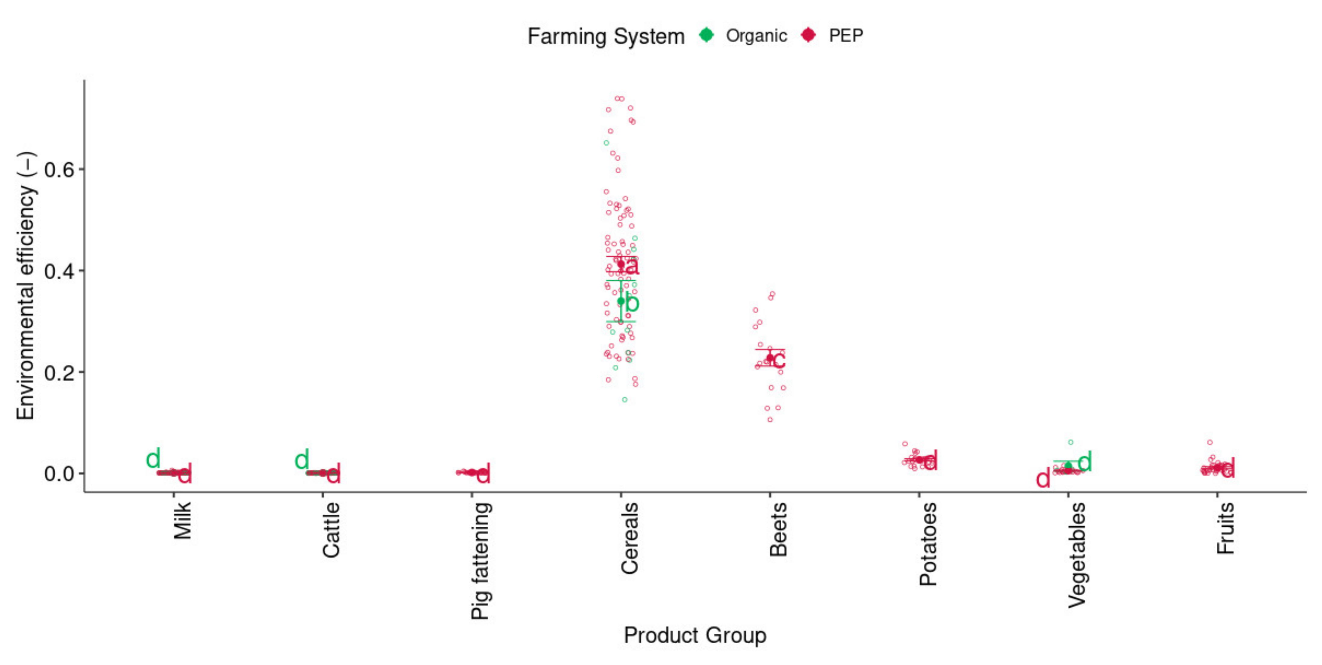
Figure A6, the different product groups differed up to an order of magnitude in their environmental efficiency. We found the lowest average environmental efficiency for the animal product groups, followed by Vegetables and Fruits, Potatoes, Beets, and Cereals. With regard to the low environmental efficiency of the product group Vegetables and Fruits, we have to consider that the chosen functional unit of energy does probably not reflect the main function of these product groups.
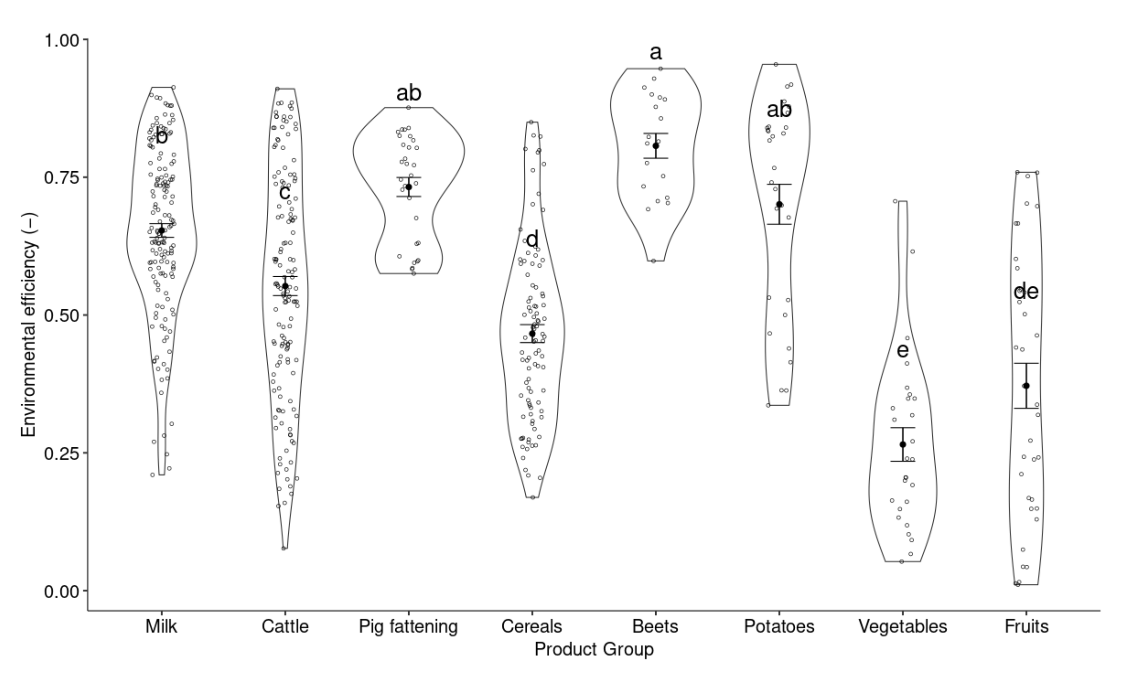
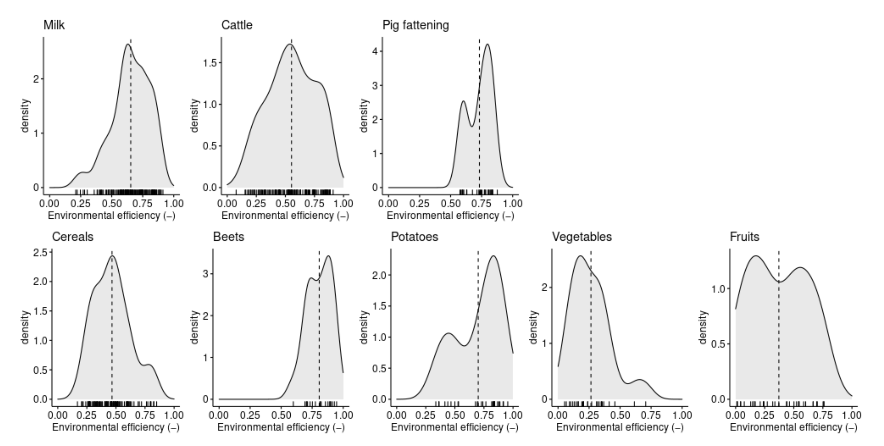
Figure A6.
“Environmental efficiency”: Observations, product group means and standard errors and ANOVA results. Significant differences in mean values between product groups are marked with distinct letters.
Figure A6.
“Environmental efficiency”: Observations, product group means and standard errors and ANOVA results. Significant differences in mean values between product groups are marked with distinct letters.
Figure A7.
For each subplot, the impact described in the column title was omitted. The values on the x-axis are the original environmental efficiency scores, the value on the y-axis are the scores without the impact.
Figure A7.
For each subplot, the impact described in the column title was omitted. The values on the x-axis are the original environmental efficiency scores, the value on the y-axis are the scores without the impact.
As shown in
Appendix A,
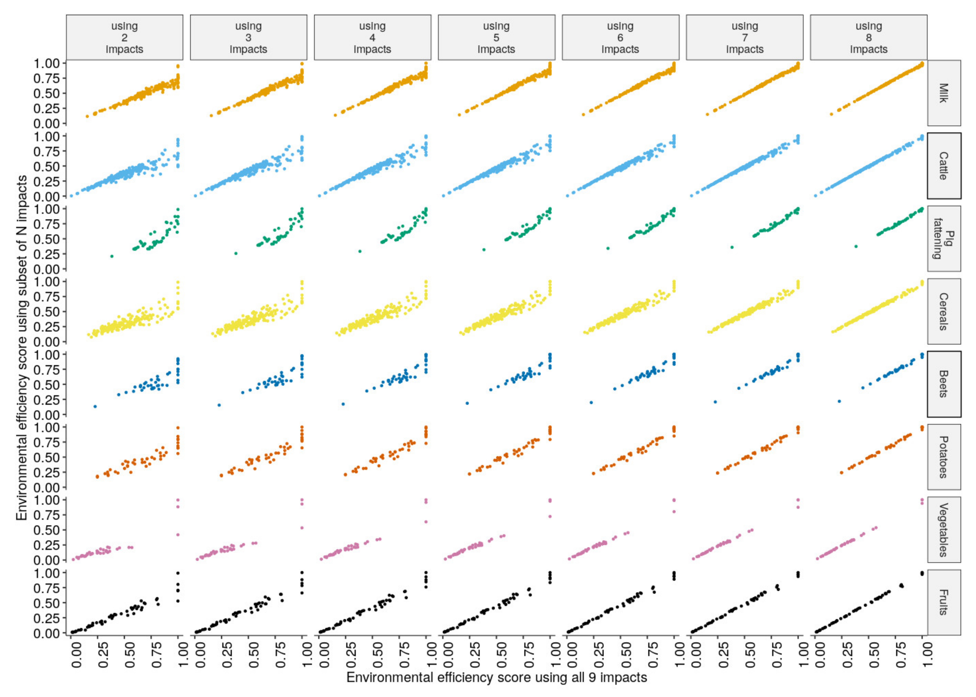
Figure A7, all impacts contribute to the environmental efficiency score, albeit not all with the same strength. Notably “IPCC GWP 100a” has only an effect on the environmental efficiency score of Milk. In order to qualify the effect of a single (omitted) impact on the environmental efficiency scores, a “leave one out” analysis was conducted. The environmental efficiency was calculated with N = one, two, three, etc. impacts omitted. Each time all possible combinations of (9–N) impacts were used to calculate the environmental efficiency and a mean was recorded. As shown in
Appendix A,
Figure A8, the number of used impacts has an effect on the environmental efficiency score.
Figure A8.
Environmental efficiency without N impacts. For each subplot, only N impacts were used. The values on the x-axis are the original environmental efficiency scores, the value on the y-axis are the scores calculated using only a subset of N impacts.
Figure A8.
Environmental efficiency without N impacts. For each subplot, only N impacts were used. The values on the x-axis are the original environmental efficiency scores, the value on the y-axis are the scores calculated using only a subset of N impacts.
Table A5.
Summary environmental efficiency scores (−).
Table A5.
Summary environmental efficiency scores (−).
| Product Group | N | Mean | Median | SD | Skew |
|---|
| Milk | 153 | 0.653 | 0.654 | 0.154 | −0.623 |
| Cattle | 143 | 0.553 | 0.551 | 0.207 | −0.134 |
| Pig fattening | 31 | 0.732 | 0.753 | 0.096 | −0.437 |
| Cereals | 97 | 0.466 | 0.461 | 0.16 | 0.487 |
| Beets | 19 | 0.807 | 0.815 | 0.098 | −0.388 |
| Potatoes | 29 | 0.701 | 0.767 | 0.195 | −0.655 |
| Vegetables | 27 | 0.265 | 0.238 | 0.158 | 1.1 |
| Fruits | 36 | 0.372 | 0.354 | 0.245 | 0.0738 |
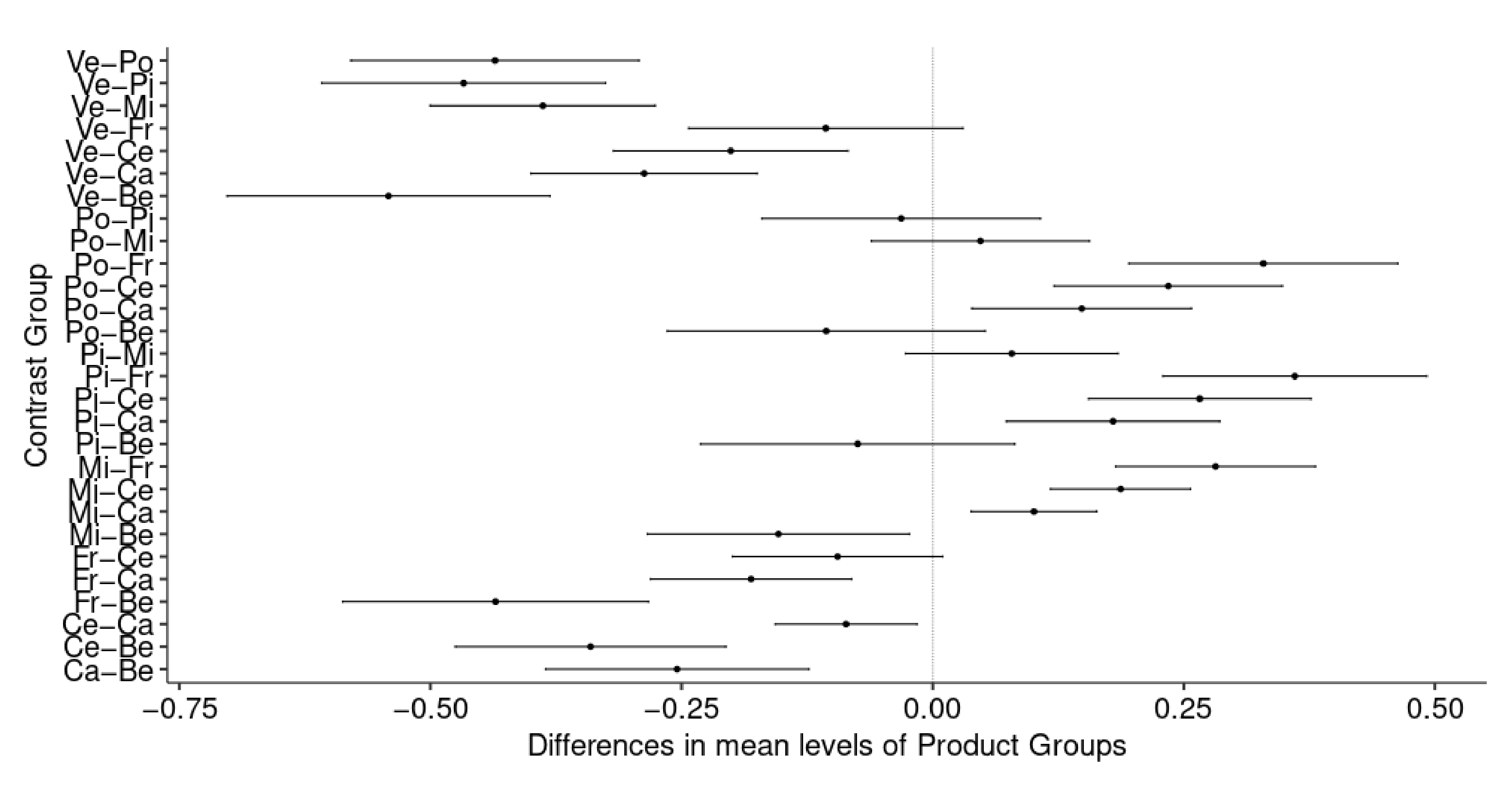
Figure A9.
Post-hoc test variance analysis: Product groups vs. environmental efficiency. Shown are the 95% confidence levels for between product group differences in mean environmental efficiency scores. The abbreviations indicate contrasting product groups: Ve = Vegetables, Pi = Pig Fattening, Mi = Milk, Fr = Fruits, Ce = Cereals, Be = Beets, Po = Potatoes, Ca = Cattle.
Table A6.
Summary one-way ANOVA environmental efficiency. The group column indicates significant differences. (i.e., the same letter indicates non–significant differences in variance, see also
Appendix A,
Figure A10).
Table A6.
Summary one-way ANOVA environmental efficiency. The group column indicates significant differences. (i.e., the same letter indicates non–significant differences in variance, see also
Appendix A,
Figure A10).
| Product Group | Mean Environmental Efficiency | Group |
|---|
| Milk | 0.653 | b |
| Cattle | 0.553 | c |
| Pig fattening | 0.732 | ab |
| Cereals | 0.466 | d |
| Beets | 0.807 | a |
| Potatoes | 0.701 | ab |
| Vegetables | 0.265 | e |
| Fruits | 0.372 | de |
Figure A10.
ANOVA Product Groups vs. environmental efficiency. The grey dots mark observations. Black dots mark mean value, error bars mark standard error. Different letters indicate a difference of means is significant at the 5% level.
Figure A10.
ANOVA Product Groups vs. environmental efficiency. The grey dots mark observations. Black dots mark mean value, error bars mark standard error. Different letters indicate a difference of means is significant at the 5% level.
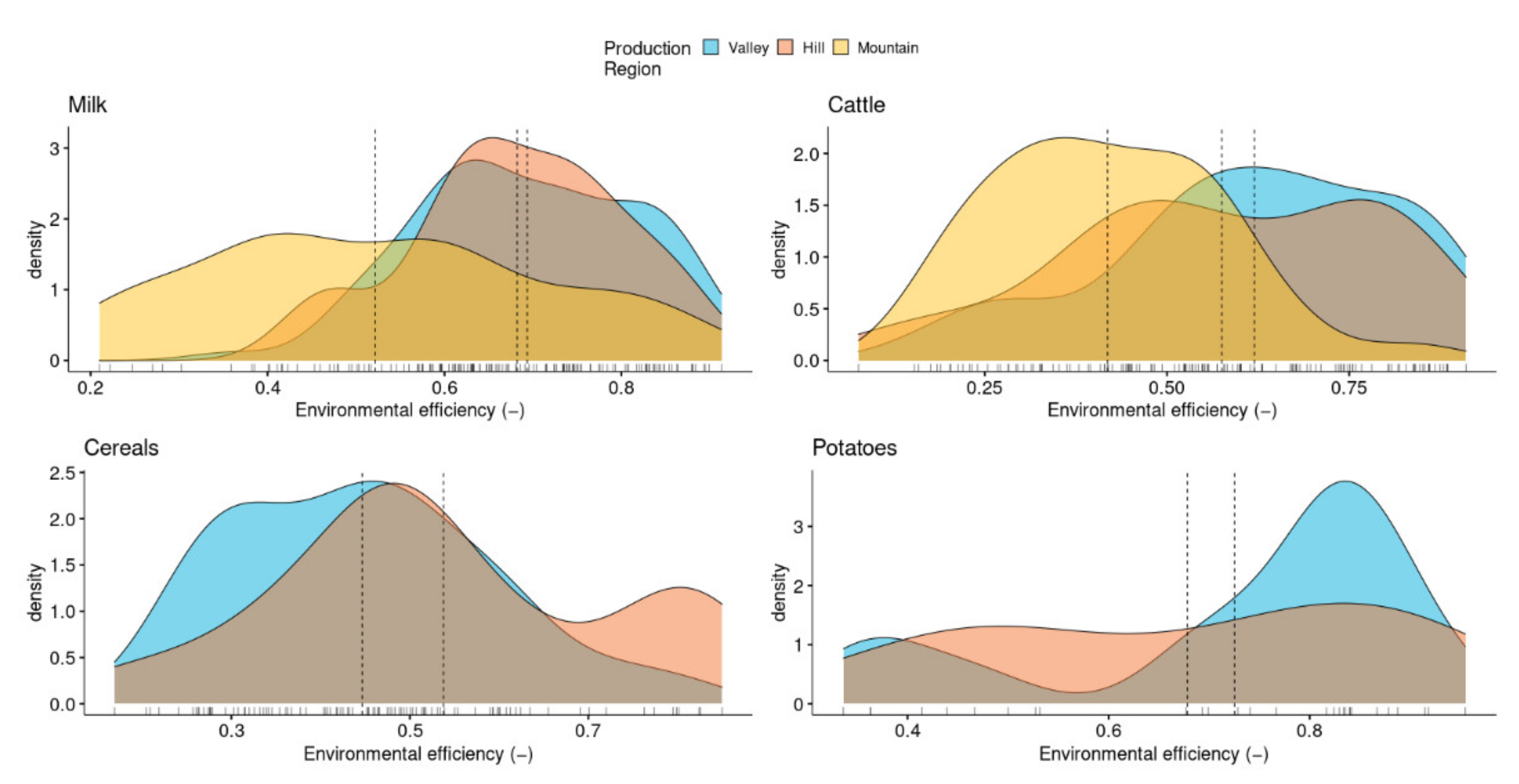
Table A7.
Summary environmental efficiency scores grouped by production-region.
Table A7.
Summary environmental efficiency scores grouped by production-region.
| Production Region | Product Group | N | Mean | Median | SD |
|---|
| Valley | Milk | 78 | 0.694 | 0.693 | 0.122 |
| Hill | Milk | 42 | 0.682 | 0.676 | 0.118 |
| Mountain | Milk | 33 | 0.522 | 0.51 | 0.191 |
| Valley | Cattle | 64 | 0.62 | 0.63 | 0.194 |
| Hill | Cattle | 40 | 0.575 | 0.59 | 0.213 |
| Mountain | Cattle | 39 | 0.418 | 0.414 | 0.155 |
| Valley | Pig fattening | 20 | 0.744 | 0.763 | 0.0842 |
| Hill | Pig fattening | 11 | 0.711 | 0.676 | 0.116 |
| Valley | Cereals | 76 | 0.447 | 0.434 | 0.146 |
| Hill | Cereals | 21 | 0.538 | 0.5 | 0.19 |
| Valley | Beets | 19 | 0.807 | 0.815 | 0.098 |
| Valley | Potatoes | 14 | 0.725 | 0.823 | 0.189 |
| Hill | Potatoes | 15 | 0.678 | 0.728 | 0.204 |
| Valley | Vegetables | 24 | 0.226 | 0.205 | 0.11 |
| Hill | Vegetables | 3 | 0.578 | 0.615 | 0.151 |
| Valley | Fruits | 22 | 0.404 | 0.404 | 0.247 |
| Hill | Fruits | 12 | 0.35 | 0.357 | 0.249 |
| Mountain | Fruits | 2 | 0.139 | 0.139 | 0.0135 |
Table A8.
Summary two-way ANOVA environmental efficiency. The group column indicates significant differences (i.e., the same letter indicates non–significant differences in variance).
Table A8.
Summary two-way ANOVA environmental efficiency. The group column indicates significant differences (i.e., the same letter indicates non–significant differences in variance).
| Contrast | N | Score | SD | Min | Max | Q25 | Q50 | Q75 | Group |
|---|
| Milk:Valley | 78 | 0.694 | 0.122 | 0.359 | 0.913 | 0.6 | 0.693 | 0.801 | abcd |
| Milk:Hill | 42 | 0.682 | 0.118 | 0.433 | 0.895 | 0.617 | 0.676 | 0.761 | abcd |
| Milk:Mountain | 33 | 0.522 | 0.191 | 0.21 | 0.88 | 0.401 | 0.51 | 0.622 | de |
| Cattle:Valley | 64 | 0.62 | 0.194 | 0.153 | 0.91 | 0.52 | 0.63 | 0.776 | bcd |
| Cattle:Hill | 40 | 0.575 | 0.213 | 0.0767 | 0.885 | 0.442 | 0.59 | 0.752 | cde |
| Cattle:Mountain | 39 | 0.418 | 0.155 | 0.159 | 0.841 | 0.309 | 0.414 | 0.543 | e |
| Pig fattening:Valley | 20 | 0.744 | 0.0842 | 0.595 | 0.876 | 0.724 | 0.763 | 0.803 | ab |
| Pig fattening:Hill | 11 | 0.711 | 0.116 | 0.575 | 0.839 | 0.607 | 0.676 | 0.828 | abcd |
| Cereals:Valley | 76 | 0.447 | 0.146 | 0.205 | 0.824 | 0.324 | 0.434 | 0.533 | e |
| Cereals:Hill | 21 | 0.538 | 0.19 | 0.169 | 0.85 | 0.454 | 0.5 | 0.655 | cde |
| Beets:Valley | 19 | 0.807 | 0.098 | 0.598 | 0.947 | 0.723 | 0.815 | 0.893 | a |
| Potatoes:Valley | 14 | 0.725 | 0.189 | 0.363 | 0.918 | 0.695 | 0.823 | 0.838 | abc |
| Potatoes:Hill | 15 | 0.678 | 0.204 | 0.336 | 0.955 | 0.514 | 0.728 | 0.854 | abcd |
| Vegetables:Valley | 24 | 0.226 | 0.11 | 0.0527 | 0.458 | 0.144 | 0.205 | 0.321 | e |
| Vegetables:Hill | 3 | 0.578 | 0.151 | 0.412 | 0.707 | 0.514 | 0.615 | 0.661 | bcde |
| Fruits:Valley | 22 | 0.404 | 0.247 | 0.0107 | 0.759 | 0.239 | 0.404 | 0.587 | e |
| Fruits:Hill | 12 | 0.35 | 0.249 | 0.0428 | 0.697 | 0.143 | 0.357 | 0.556 | e |
| Fruits:Mountain | 2 | 0.139 | 0.0135 | 0.129 | 0.148 | 0.134 | 0.139 | 0.144 | e |
Table A9.
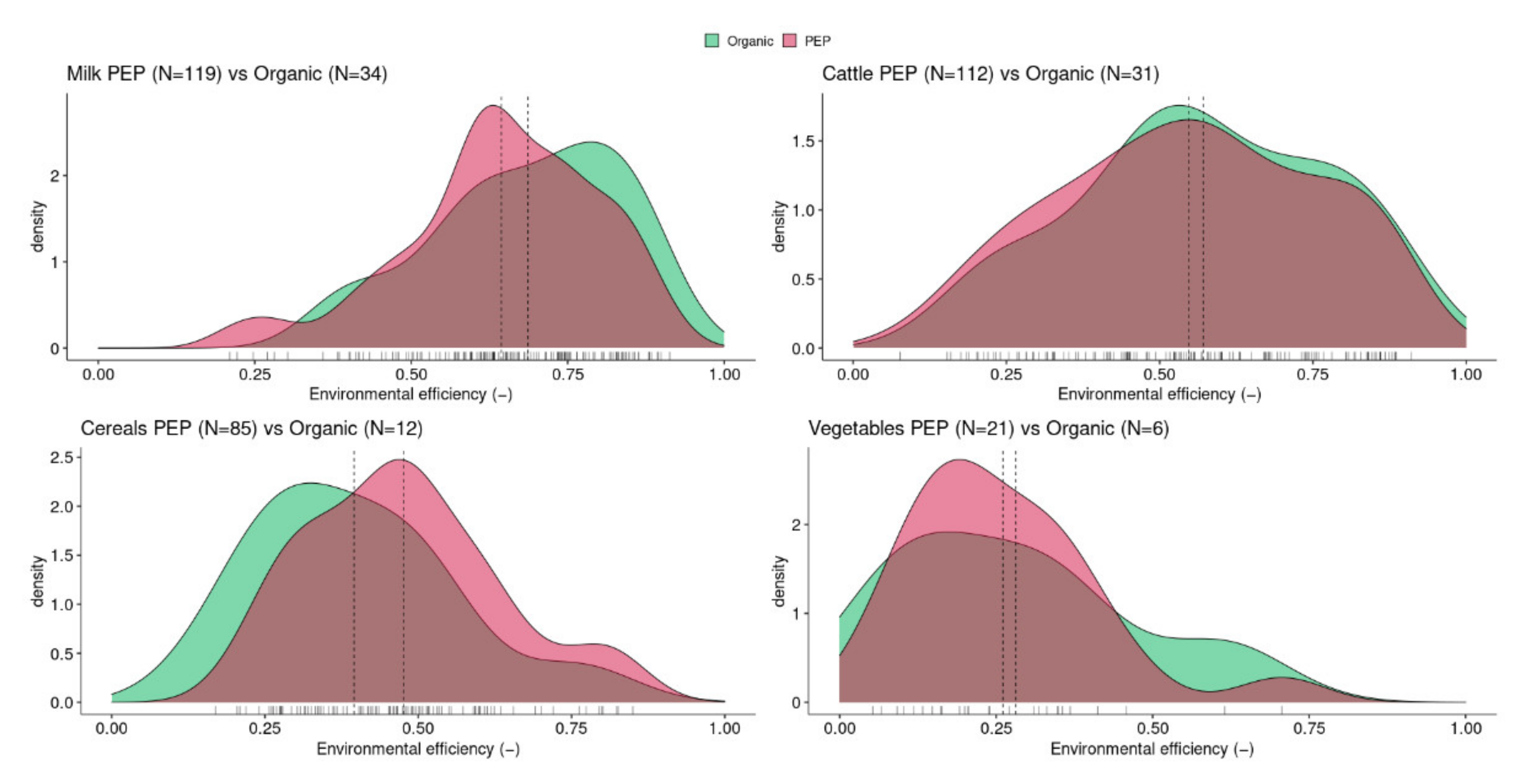
Summary environmental efficiency scores proof of ecological performance (PEP) and Organic farming. The column “p.val” shows the p-value from an ANOVA.
Table A9.
Summary environmental efficiency scores proof of ecological performance (PEP) and Organic farming. The column “p.val” shows the p-value from an ANOVA.
| Product Group | Farming System | N | Mean | Median | Sd | p.Val |
|---|
| Milk | Organic | 34 | 0.686 | 0.725 | 0.149 | 0.159 |
| Milk | PEP | 119 | 0.644 | 0.651 | 0.155 | 0.159 |
| Cattle | Organic | 31 | 0.571 | 0.551 | 0.2 | 0.578 |
| Cattle | PEP | 112 | 0.547 | 0.552 | 0.209 | 0.578 |
| Cereals | Organic | 12 | 0.395 | 0.37 | 0.164 | 0.825 |
| Cereals | PEP | 85 | 0.476 | 0.466 | 0.158 | 0.825 |
| Potatoes | Organic | 4 | 0.721 | 0.759 | 0.151 | 0.102 |
| Potatoes | PEP | 25 | 0.698 | 0.767 | 0.203 | 0.102 |
| Vegetables | Organic | 6 | 0.281 | 0.259 | 0.2 | 0.787 |
| Vegetables | PEP | 21 | 0.261 | 0.238 | 0.15 | 0.787 |
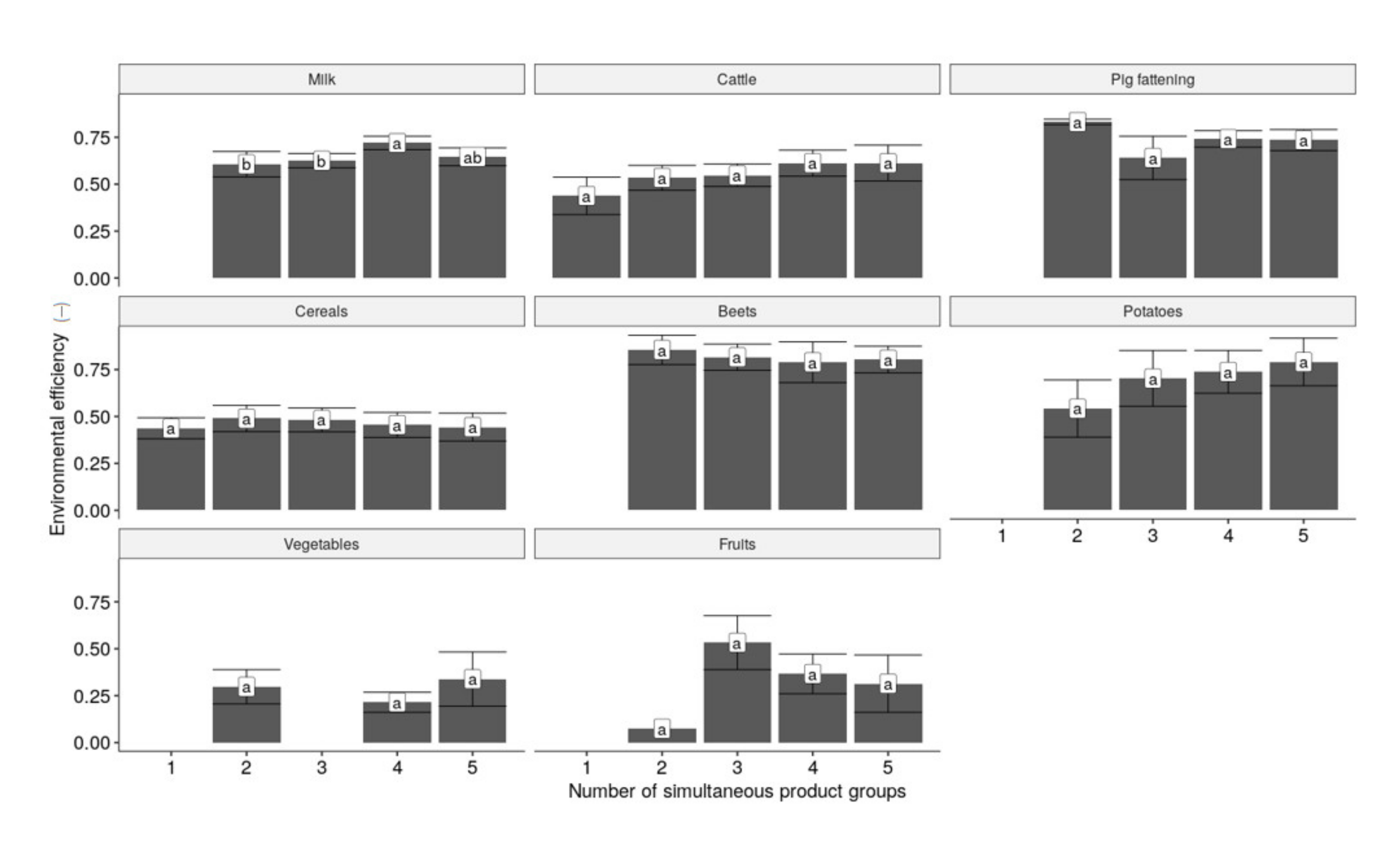
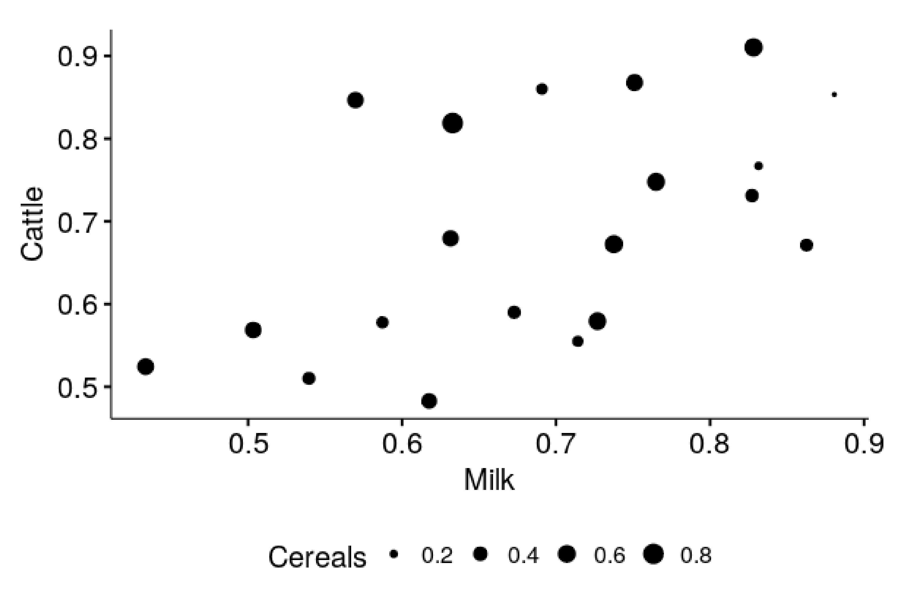
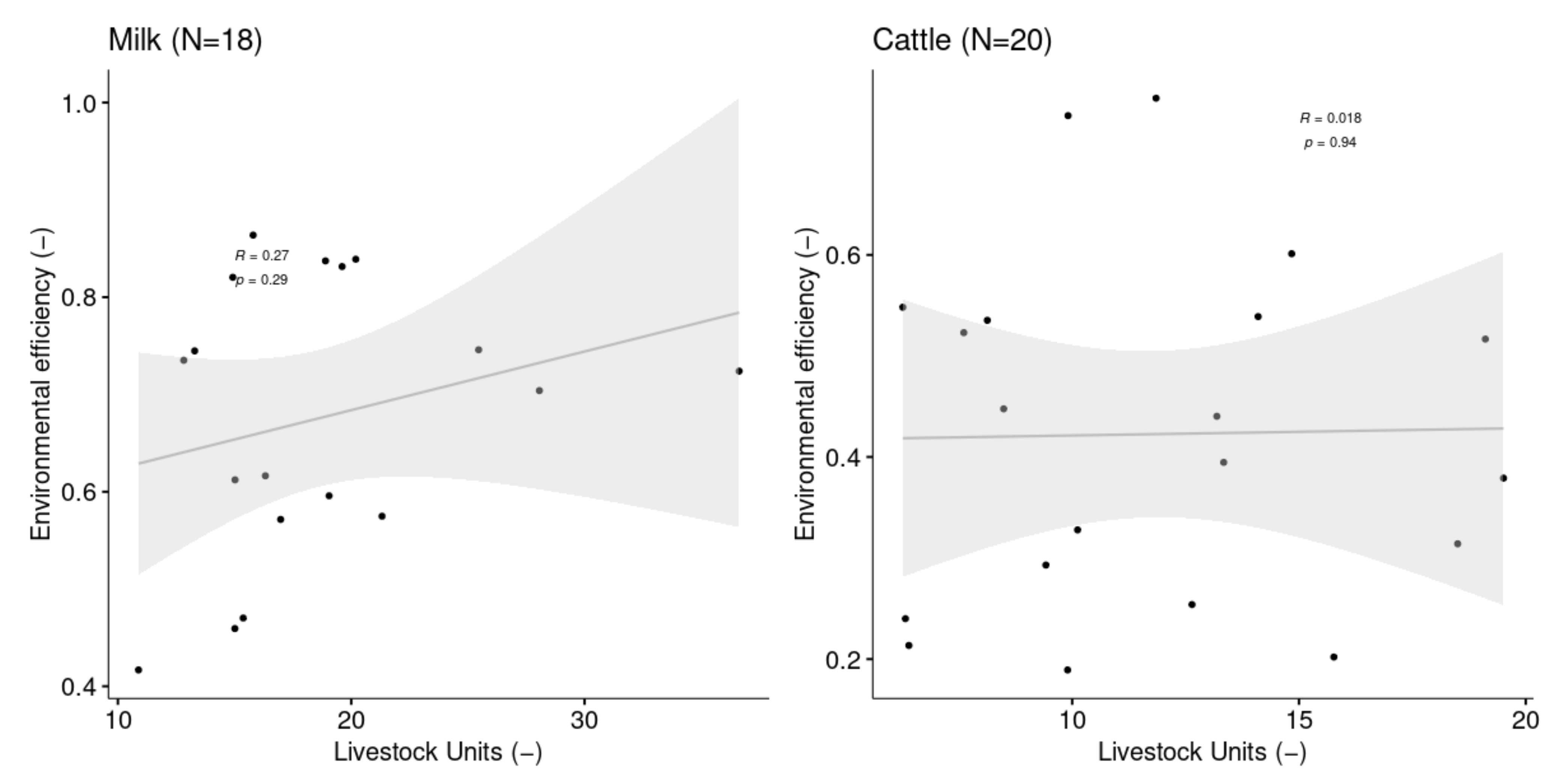
Figure A11.
Environmental efficiency for farms with multiple product groups (mixed farms). Farms, where multiple product groups are larger than 33% of the average product group size (see
Appendix A), were considered as ‘mixed’ or ‘specialized’ farms. Shown are only farms, which have the three product groups “Milk”, “Cattle breeding”, “Cereals” simultaneously (N = 20). The
x-axis shows the size of the product group in Livestock units for animal product groups and hectares for crops. The grey area around the regression line marks the 95% confidence interval. Additionally, the regression coefficient (R) and its
p-value (
p) are shown.
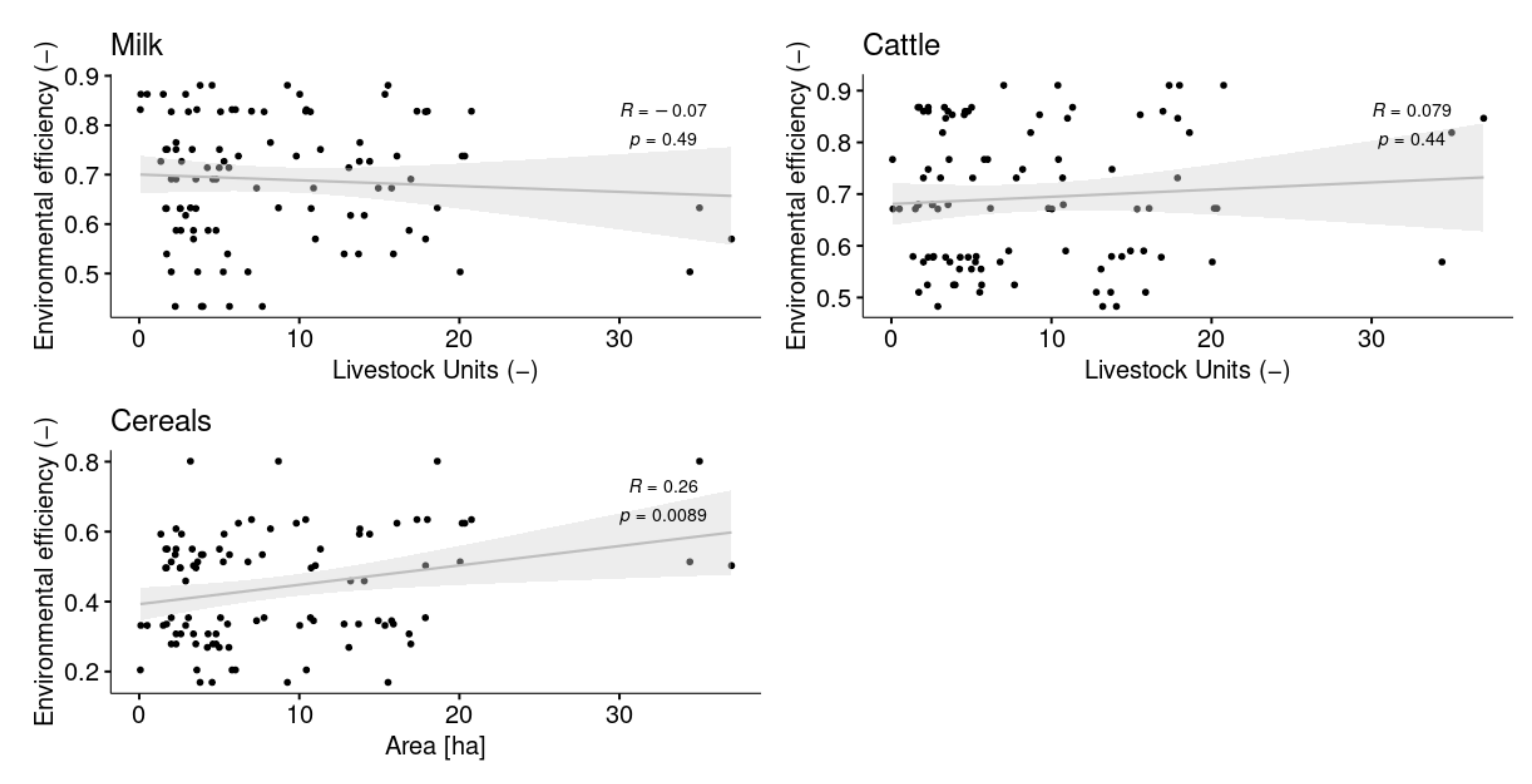
Figure A12.
Environmental efficiency for farms with only one (dominant) product group. Farms with all other product groups smaller than 33% of the average product group size (see
Appendix A) were considered as ‘non-mixed’ or ‘specialized’ farms. The
x-axis shows the size of the product group in Livestock units for animal product groups and hectares for crops. The grey area around the regression line marks the 95% confidence interval. Additionally, the regression coefficient (R) and its
p-value (
p) are shown.
Table A10.
Correlation coefficients (p-value) for mixed farms product group environmental efficiency.
Table A10.
Correlation coefficients (p-value) for mixed farms product group environmental efficiency.
| | Cattle | Milk | Cereals |
|---|
| Cattle | 1 (0) | 0.545 (0.013) | 0.124 (0.601) |
| Milk | 0.545 (0.013) | 1 (0) | −0.247 (0.295) |
| Cereals | 0.124 (0.601) | −0.247 (0.295) | 1 (0) |


