Article

Assessment of Weed Classification Using Hyperspectral Reflectance and Optimal Multispectral UAV Imagery

1
School of Agriculture and Food Sciences, The University of Queensland, Gatton Campus, QLD 4343, Australia
2
Department of Agriculture Technology, Faculty of Agriculture, University Putra Malaysia, Serdang 43400, Selangor, Malaysia
*
Author to whom correspondence should be addressed.
Agronomy 2021, 11(7), 1435; https://doi.org/10.3390/agronomy11071435
Submission received: 29 May 2021 / Revised: 7 July 2021 / Accepted: 16 July 2021 / Published: 19 July 2021

Abstract

:
Weeds compete with crops and are hard to differentiate and identify due to their similarities in color, shape, and size. In this study, the weed species present in sorghum (sorghum bicolor (L.) Moench) fields, such as amaranth (Amaranthus macrocarpus), pigweed (Portulaca oleracea), mallow weed (Malva sp.), nutgrass (Cyperus rotundus), liver seed grass (Urochoa panicoides), and Bellive (Ipomea plebeian), were discriminated using hyperspectral data and were detected and analyzed using multispectral images. Discriminant analysis (DA) was used to identify the most significant spectral bands in order to discriminate weeds from sorghum using hyperspectral data. The results demonstrated good separation accuracy for Amaranthus macrocarpus, Urochoa panicoides, Malva sp., Cyperus rotundus, and Sorghum bicolor (L.) Moench at 440, 560, 680, 710, 720, and 850 nm. Later, the multispectral images of these six bands were collected to detect weeds in the sorghum crop fields using object-based image analysis (OBIA). The results showed that the differences between sorghum and weed species were detectable using the six selected bands, with data collected using an unmanned aerial vehicle. Here, the highest spatial resolution had the highest accuracy for weed detection. It was concluded that each weed was successfully discriminated using hyperspectral data and was detectable using multispectral data with higher spatial resolution.

1. Introduction

Weeds are unwanted plants that can damage and reduce crop yields, becoming worse over time if no action is taken to control the growth rate of the weeds. The competition for moisture, nutrients, and sunlight between the weeds and crops affects crop yields, which can be reduced by 45–95% [1,2,3]. The use of chemicals is widespread because of their effectiveness.; however, because of the diversity of weed and due to herbicide resistance [4], this is not a long-term solution. The excessive use of herbicides harms crops and increases the end product price [3], in addition to jeopardizing environmental protection efforts [4] and leading to soil contamination [5], unless natural herbicides made of organic acids or essential oils are employed to mitigate these negative impacts; however, organic herbicides can be expensive.
As such, spot spraying can reduce the amounts of herbicides to which the crops are exposed. This method is used to prevent weeds from affecting the crops [6]. This is better than blanket application using the site-specific weed management (SSWM) approach, in which the herbicide is sprayed on only a few spots in the field according to the patch area at an exact location and exact time [7]. This method is used to identify the locations of the weed patches and the weed species [8].
The SSWM method uses statistical analysis to differentiate weeds from crops [9]. With the SSWM method, information is collected using remote sensing, whereby the spectral wavelengths are detected for each plant [10]. One of the spectral analysis methods used to discriminate between winter (wheat and clover) and summer (maize and rice) crops is linear discriminant analysis (LDA) [11]. For instance, the spectral signatures of wheat range from 350 to 712, 451 to 1562, and 1951 to 2349 nm. In comparison to wheat, clover has spectral signatures in the range of 727 to 1299 nm. The spectral signatures for maize are similar to those of rice and almost the same as wheat, at 350 to 713, 1451 to 1532, and 1951 to 2349 nm. It has been proven that each plant or crop has unique spectral signatures and wavelength bands.
Many statistical analysis methods are used to process hyperspectral data, including stepwise linear discriminant analysis (SLDA), principal component analysis (PCA), support vector machine (SVM), random forest (RF), neural network (NN), and linear discriminant analysis (LDA) approaches. STEPWISE was created based on these approaches. The RF and SVM models were tested in terms of their hyperspectral data with feature selection using a successive projection algorithm (SPA). Based on the SPA selection, the results showed more than 90% classification accuracy for barnyard grass, weedy rice, and rice using a SVM with six spectral bands (415, 561, 687, 705, 735, and 1007 nm) [12]. The neural network machine learning algorithm successfully classified herbicide-resistant weeds at 25% to 79% accuracy using an unmanned aerial vehicle (UAV) [13]. The results depended on the sunlight, images, and growth stage of the plants. Linear discriminate analysis (LDA) and support vector machine (SVM) classifiers are the best techniques for weed classification, with 90% and 87.14% accuracy, respectively [14]. The same goes for LDA in classifying lettuce varieties, providing 81.04% accuracy [15]. This shows that the plants’ spectral signatures can be used for classification, which can be improved using UAV image processing.
It is challenging to process the resulting images due to the similarities between weeds and crops; thus, object-based image analysis (OBIA) can be used to segment features based on the objects in an image. The combination of k-means and multiresolution segmentation OBIA can be used to differentiate weed species [16]. The segmentation is performed based on the textures, objects, and color features [16]. UAV imagery enables data collection for weed mapping using the random forest–OBIA method. Farmers can use weed maps to manage their fields [6].
In this study, aimed to find out whether hyperspectral data can be used to discriminate weeds from crops. Our hypothesis was that hyperspectral data would be able to help in identifying weeds by using the spectral bands to detect the weeds in the field; therefore, the hyperspectral analysis of weed species in sorghum crops was explored. The aim was to discover the significant spectral bands that can be used to discriminate weeds species and how the spectral bands can be used to detect weeds within fields. The data were classified using statistical analysis and image processing. Then, the significant spectral bands were used to detect weeds in the field using multispectral UAV data. If weeds are detectable using image processing, this will help farmers to monitor weeds at earlier stages to avoid weed infestation, meaning farmers will be able to only spray the weed patches in the affected areas, reducing costs and protecting the soil and crops from excessive chemicals.

2. Materials and Methods
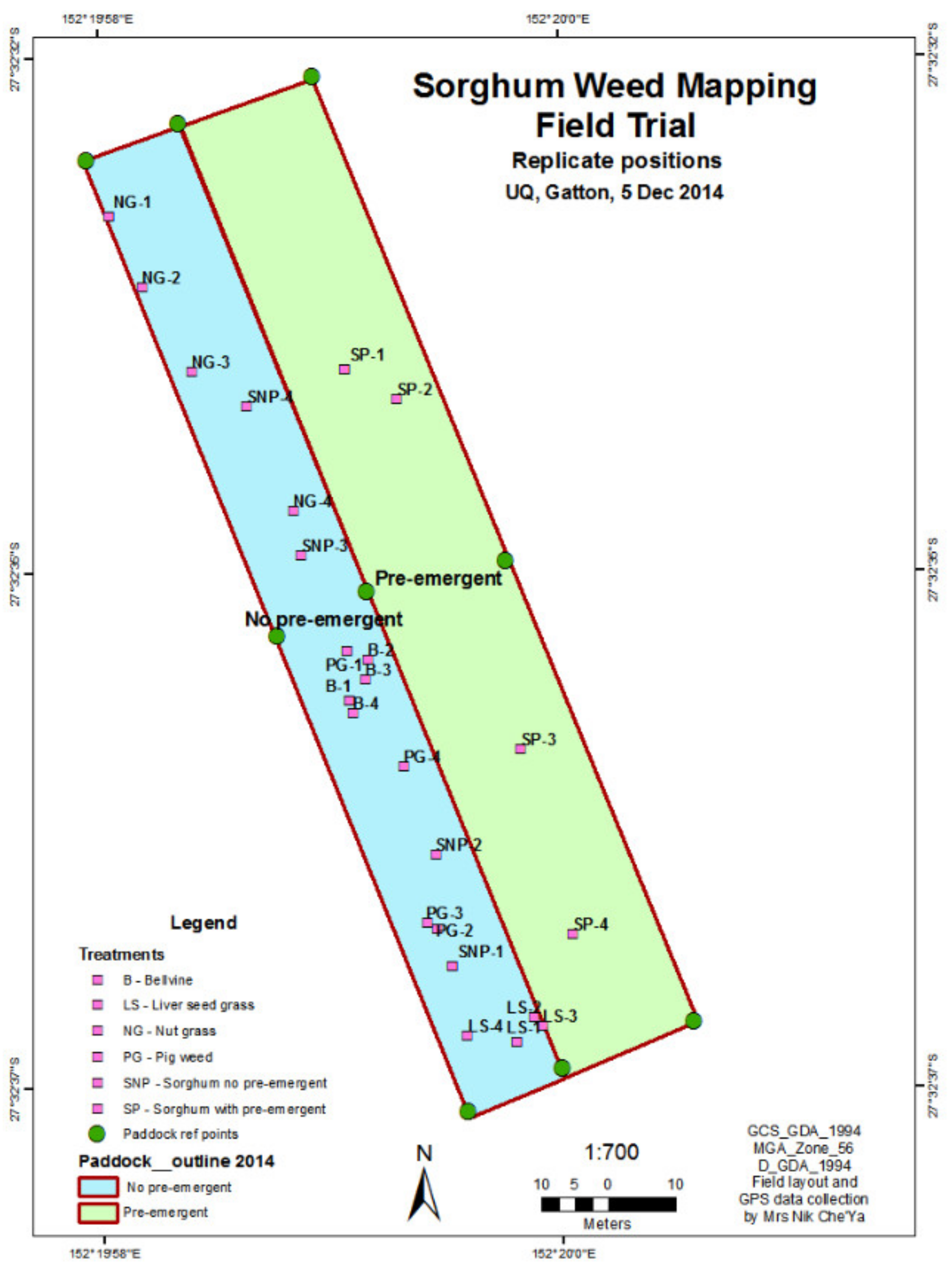
2.1. Site Data

This study was conducted at the Gatton Campus, Queensland (27°32′32.90″ S, 152°19′58.88″ E, WGS 84 Datum) (Figure 1). During the summer, Sorghum bicolor (L.) Moench (SG) variety 84G22 was used to detect weeds in the research area. The seeds were placed in the ground using the StarFire integrated terrain compensation (iTC) global positioning system (GPS) tractor at 30 mm depth on 25th October 2013 and 26th November 2014. The crop rows for sorghum were set at 75 cm using a Case IH 95 tractor fitted with a four-unit Nodet planter.
The experimental design used in this study involved a 6 × 4 randomized block design. The plots of those treated with control (untreated) and pre-emergence herbicide were separated. Two pre-emergence herbicides were used, namely Gesaprim® 600 SC at a rate of 2 L/ha (with 600 g/L atrazine active constituent) and DualGold® at a rate of 2 L/ha (with 960 g/L S-metolachlor active constituent).
Sorghum species were placed in each plot. In this study, one type of sorghum species was placed in each quadrat. The four replicates were placed randomly. In this condition, we focused on the common weed species and those highlighted in Table 1.

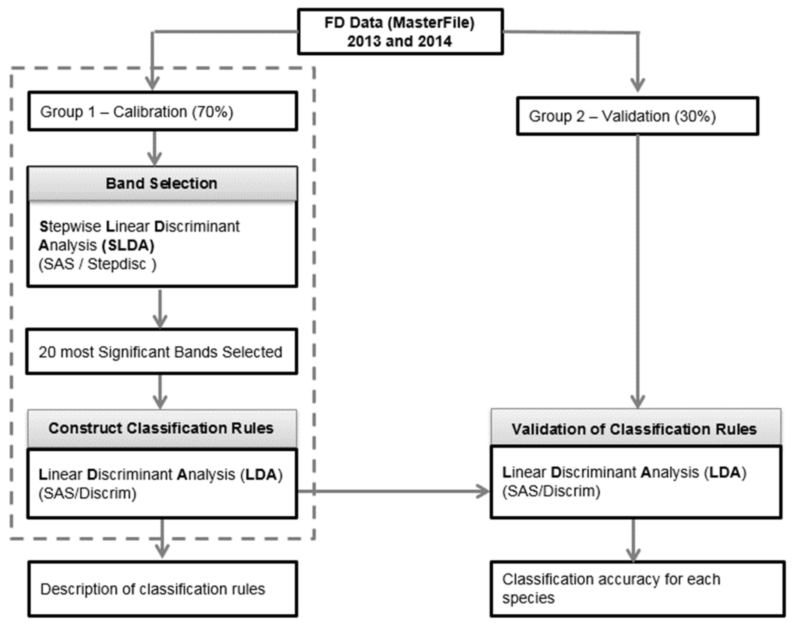
2.2. Spectral Separability Procedures

The hyperspectral data in the range of 325–1075 nm were collected using the ASD FieldSpec® HandHeld 2 spectroradiometer (Malvern Panalytival, Cambridge, United Kingdom (U.K)). This instrument is a minimal, convenient, visible near-infrared (VNIR) alternative to the ASD FieldSpec 4 [17]. The ASD FieldSpec® HandHeld 2 spectroradiometer is a robust and sturdy device that uses the ASD FieldSpec 4 VNIR spectrometer for efficient measurement [17]. The data for each weed species and sorghum crop were collected in 2013 and 2014. Data collection started from week two and continued until week four at different growth stages of the weeds and crops. The optical panel was calibrated using white references. Prior to measurement, the ASD FieldSpec® HandHeld 2 spectroradiometer was calibrated with a Spectralon white reference panel provided by the manufacturer (Malvern Panalytival, Cambridge, United Kingdom (U.K))., as indicated in the operation guide [18]. ASD FieldSpec® HandHeld 2 instrument was aimed so that the optical input was shown but did not darken the white reference panel, while being close enough for the panel to fill the field of view. It was important to conduct a calibration process before and after hyperspectral data were collected for optimization and dark current collection. Each spectral signature of the leaves was collected. Then, the data were transferred to a computer and saved in MasterFile format. The MasterFile data were binned and run using the first derivative (FD) analysis.

Classification Procedures

The data were split into calibration data (group 1, 70%) and validation data (group 2, 30%) (Figure 2) [14]. The calibration and validation data were randomly split into two groups.
Stepwise linear discriminant analysis (SLDA) was run to identify 20 significant bands in the calibration data via the STEPDISC procedure using SAS (SAS Institute, North Carolina State University, United States of America (USA)) software. The linear discriminant analysis was constructed using the “rule set” from the 20 significant bands. Then, the validation data were run with the same “rule set” to verify the accuracy.

2.3. Band Identification

The identified bands were combined into six bands because the multispectral sensor MCA 6 (Tetracam Inc., California (USA)) can only be fitted with six bands; therefore, in this paper, only six bands are shown. The best six-band combinations were chosen from the eight bands (from the currently available MCA 6 (Tetracam Inc., California (USA)), with another six bands from the 20 significant bands (Table 2). The MCA 6 multispectral camera was used to collect the aerial images in the sorghum field using UAV. For the MCA 6 camera, only six bands were used during the flight (because the sensor could only be fitted with six bands). The combination of the eight bands was used because produced more combinations; thus, to find the best six bands, the band combinations were run using discriminant analysis to obtain the highest classification accuracy. Almost all spectral regions resembled those from MCA 6 and the six bands from the 20 significant bands (using linear discriminant analysis (LDA)); however, for the red-edge region, MCA 6 highlighted bands at 750, 730, 720, and 710 nm, while LDA only highlighted bands at 720 and 710 nm.

2.4. Multispectral Imagery Data Collection

The MikroKopter JR11X UAV and multiple camera array 6 (MCA 6) sensor (Tetracam Inc., California (USA)) were used to collect the aerial images at week 3 (17 December 2014). The MCA 6 camera has six sensors that can be fitted in the UAV. The six bands were chosen based on the results in Section 2.3. The multispectral data were collected for different spatial resolutions, which were 5.43 mm (flight height: 10 m), 10.83 mm (flight height: 20 m), and 20.31 mm (flight height: 37.5 m). The RGB imagery was collected at a height of 1.6 m (0.87 mm spatial resolution). The field of view (FOV) for MCA 6 was 38.3° × 31.0°. The image size was 1280 × 1024. The advantages of MCA 6 are that it can provide 8 or 10 bit data and its weight of 790 g enables it to be attached to UAVs.

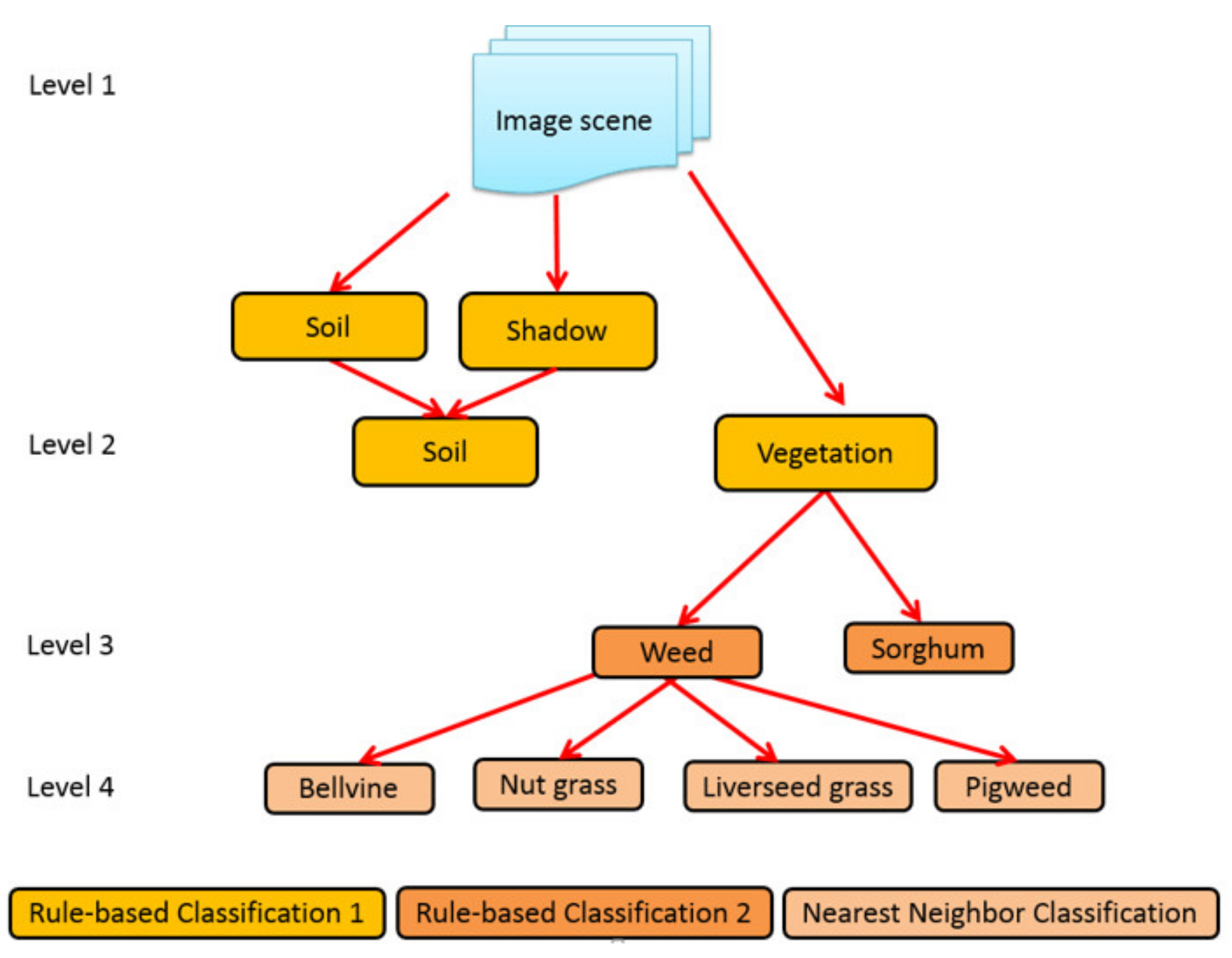
2.5. Object Based Image Analysis (OBIA) Procedures

The images were segmented and classified using the nearest neighbor (NN) method with vegetation, soil, and shadow samples. The OBIA workflow is shown in Figure 3. This shows the hierarchy level for the whole image, which is then narrowed down to the vegetation, before being dividing it into two classes in level 3. In level 4, there are four types of weed.
The image segmentation started at the scale of 40, using the “multiresolution segmentation” algorithm, based on the color (spectral) and shape or the spatial criterion (Figure 4). In this study, the spectral and shape values were weighted based on their homogeneity. The shape value was 0.1 because the overall shape of the weeds and sorghum was only ten percent of the total, which led to inaccurate segmentation. The color value (wcolour) was 0.5 because the spectral bands of the weeds and sorghum were similar, with only slight differences. The compactness values indicated different shapes and smoothness weights, showing variability in terms of features. The parameters values were flexible because they were based on trial and error.
The objects were classified according to soil (SO) and vegetation, then the vegetation was segmented on a scale of 1 to 10. In fact, the vegetation was divided into sorghum and weeds. Then, both sorghum and weeds were reclassified. Using the “enclosed by class” function, sorghum was merged while weeds were split into different classes. This rule set can be slightly modified to run other images and data.
The confusion matrix was used to assess the accuracy before its adoption as a normal procedure [19,20,21,22]. The KHAT statistic was computed based on [23] as:
N i = 1 r x i i i = 1 r x i +   *   x + i N i = 1 r x i +   *   x + i
where r is the number of rows in the matrix; xii is the number of observations of row i and column i; xi+ and x+i are the marginal total of row i and column i, respectively; N is the total number of observations.

3. Results and Discussion

3.1. Classification of Weeds Species

Weeds can be discriminated using stepwise linear discriminant analysis (SLDA), and the classification of the validation data in 2013 was 85–90% accurate, as illustrated in Table 3. Stepwise linear discriminant analysis was used in lettuce varieties, showing a classification accuracy of 81.04% [15]. These results can be improved using high-dimensional analysis methods, such as a support vector machine (SVM) [12,24].
Table 4 shows that the validation data in 2014 were 97–100% accurate. This means that the accuracy increased from the previous year and the results shown were consistent.

3.2. Classification and Validation

The significant bands for the classification of weeds and sorghum were successfully analyzed using linear discriminant analysis (LDA). In 2013, the significant bands were tested for their classification accuracy. The accuracy of Malva sp. (MW) decreased to 90%, while sorghum reached more than 90% accuracy in week two (Table 3, calibration section). This shows that the classification accuracy was high (>80%). Meanwhile, the sorghum accuracy increased to 92% in week three, then finally all weeds showed 100% classification accuracy during week four. Here, the larger the size of the weeds, the more accurate the classification.
The weed classification was tested using independent data (Table 3, validation section). In week two, the classification accuracy for sorghum increased to 70%, reaching 75% in week three; however, it decreased to 4% during week four in 2013. The same was true for Malva sp. (MW), where the classification was 75% accurate in week two but increased to 100% in weeks three and four. The accuracy for Amaranthus macrocarpus (AM) decreased to 80% in week three, although for Urochoa panicoides (LS) remained at 100% from week two to week four. Although the accuracy of Cyperus rotundus (NG) decreased from 100% to 67% in week three, it improved by up to 100% in week four. The classification accuracy decreased by 3–4% in week four for sorghum. Overall, the results proved that the classification improved from week two to week four in 2013. In 2014, the classification was 100% successful for most of the significant bands for each week (both calibration and validation data), except for the 89% classification accuracy for Urochoa panicoides (LS) in week two.
The independent data tested in 2013 using linear discriminant analysis (LDA) produced accurate results, as highlighted in Table 3. Meanwhile, stepwise linear discriminant analysis (SLDA) was used to test the dependent data and the classification accuracy was found to be slightly lower. The classification accuracy increased to 100% in 2014 using SLDA, as shown in Table 4. The accuracy of the classification for the weed discrimination using LDA and support vector machine (SVM) has been increased at 15 bands compared to the eight bands at more than 90% and 85%, respectively [24]. Similar results were found for the separation between weed species using LDA, which has a high degree of separation [25]. A previous study found that discriminant analysis (DA) can detect grass and broadleaf weed species with 70 to 100% accuracy [26].
The differences in the classification between weeds and sorghum in 2013 and 2014 were insignificant. The statistical analysis showed that most of the classification was at 100% for both years. Additionally, the different growth stages between week two and week four were not prominent. Weed discrimination with other species was investigated during pre-planting and found the overall accuracy above 95% [25]. It is of excellent significance to increase weed identification accuracy for pre-planting applications. The differences in results seen here were influenced by the growth stages and locations of the plants, as well as abiotic and biotic parameters [27]. Additionally, the spectral reflectance of plants depends on the weather conditions and the amount of sunlight received, due to the atmospheric conditions and azimuth [28]. The plants’ morphology also affects their spectral reflectance, such as the shape and color of the leaves. These similar findings suggest that the environmental factors, microclimates, plant leaves, solar angles, and changing morphological and spectral properties are different at every growth stage, which will influence weed detection [29]. Humans are unable to differentiate between these plants features using the naked eye; thus, by using spectral signatures, the plants can be differentiated and classified using statistical analysis and machine learning [30,31,32].
A previous study showed that linear discriminant analysis (LDA) is more accurate compared to principal component analysis (PCA) in classifying Sesbania herbacea (Mill.) McVaugh (hemp sesbania), Ipomoea wrightii (palm leaf morning glory), Ipomoea lacunosa (pitted morning glory), Sida spinosa (prickly sida), Senna obtusifolia (sicklepod), and Jacquemontia tamnifolia (small flower morning glory) species in soybeans [33]. A similar study found that weeds and wheat were successfully classified with 100% accuracy using partial least squares (PLS) analysis and linear discriminant analysis (LDA) [34]. The short-wave infrared (SWIR) wavelengths between 1445 and 2135 nm were used in the previous study. Compared to our study, wavelengths of up to 1000 nm were used; thus, in the future, it is recommended to use SWIR wavelengths for weed classification. In a study in New Zealand, hyperspectral imaging was used to detect weeds using machine learning (ML). This method was another way of detecting weeds quickly and accurately using the multilayer perceptron method at 89% accuracy [26]; thus, hyperspectral imaging can be used in weed detection using ML as compared to object-based image analysis.

3.3. Band Identification

The results showed that the highest accuracy for the six combinations was 93%, involving the combination of the bands at 440, 560, 680, 710, 720, and 850 nm. The linear discriminant analysis (LDA) results from the hyperspectral data were significant for the six combinations. Table 5 shows the results from the classification of band combinations based on Table 2. There were 28 combinations (please refer to [14]), although only three are highlighted in in Table 5. The band combinations were narrowed down into five-, four-, and three-band combinations. The combination results can be found in [14].
The spectral signatures showed that each plant had significant bands. Based on the spectral signatures, each weed species in the sorghum field was identified. The band combinations helped us to more accurately identify the weeds in the sorghum field. The 20 significant bands were narrowed down to eight bands, which were used in the multispectral sensor. This method was similar to the previous research, in which the bands underwent further analysis [35]. The discrimination accuracy between sugar beets and maize was 90% when using specific spectral bands [36].
A similar study used spectral signatures (500–550, 650–750, 1300–1450, and 1800–1900 nm) to successfully discriminate weeds from sugarcane [30,32]. The short-wave infrared bands (SWIR; 1660, 1890, and 2000 nm) matched the primary features of the pure cellulose and lignin spectra of the plants. Changes in cellulose and leaf water content determine the levels of these characteristics, which can be leveraged to classify plant species [30]. Several wavelengths, including 491, 541, 641, 722, 772, 852, 942, 1047, 1132, 1443, and 2475 nm, were selected and calculated for the purpose of identifying plants species using an artificial neural network (ANN) and support vector machine (SVM) [31]. We found that ANN and SVM provided high levels of accuracy of up to 86%.
Other examples were the wavelengths of 440, 500, 530, 550, 560, 575, 590, 620, 640, and 675 nm, which were used to classify seagrass in Southeastern Australia [2]. Similar results were found using specific wavelengths to discriminate Bermudagrass (Tifway 419). In fact, wavelengths of 353, 357, 360, 362, 366, 372, 385, 389, 391, 396, 405, 441, 442, 472, 726, 727, 732, and 733 nm were found in the discriminant analysis (DA) of Bermudagrass (Tifway 419) at 98% accuracy.
The combination of visible (VIS) and near infra-red (NIR) bands improved the classification accuracy using linear discriminant analysis (LDA) between weeds and sugar beets (686, 694, 726, 856, 897, and 970 nm), as well as between potatoes and weeds (686, 726, 856, 897, 970, and 978 nm) [37]. Furthermore, the health of the citrus crop was verified using 440, 560, 680, 710, 720, and 850 nm bands [38], consistent with the results in this study.
Mediterranean plants were found by using the high spectral resolution of the mid-infrared (MIR) radiation, enabling accurate species discrimination [39]. Since this study focused on the visible to near-infrared (325 to 1075 nm) range, we suggest that future studies should consider spectral reflectance from 1055 up to 2000 nm for further analysis of weed discrimination, because MIR reflectance is also affected by the moisture content of plants [39].

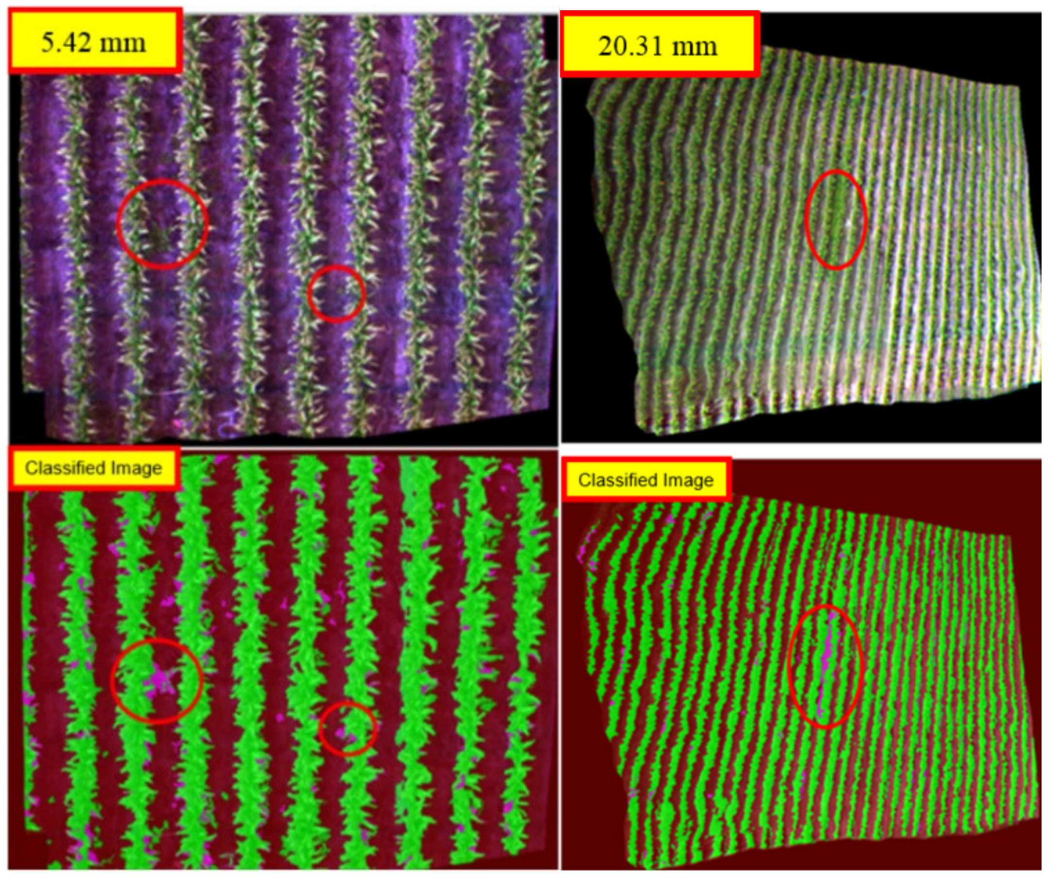
3.4. Results of Image Processing

The same six spectral bands were used for image collection in the field. The spectral, physical, and contextual characteristics of the weeds and sorghum affect the development and efficiency of the segmentation and classification rule sets in image processing procedures. The rule sets in the object-based analysis (OBIA) can be modified to identify weeds at different growth stages so that the results are more accurate. In addition, the detection of weeds will be more accurate when using a high spatial resolution.
The growth stages of the weeds from week one to week four after being planted were assessed via multispectral images. Based on the results, weeds and sorghum were accurately classified in week three (Table 6), because the sizes of both were bigger in comparison to weeks one and two; however, the size of the weeds was still small and they were easy to separate from the sorghum plants. The same was true for Cyperus rotundus (NG) and Urochoa panicoides (LG), which were successfully classified in week three after planting. The shapes of leaves such as broadleaf Portulaca oleracea (PG) and Ipomea plebeian (B) were easier to distinguish. Both were successfully classified in week three. The literature showed how grass weed seedlings were discriminated from monocotyledonous crops, with seedlings of broadleaf weeds in dicotyledonous crops proving more challenging to identify at later stages [40] because they have similar spectral reflectance and due to the spread of weeds in small patches and the effects of soil reflectance at the early stages of growth [41].
The weeds started to mix with the crop at week four; thus, the broadleaf weeds were detected at an early stage. Weed detection earlier stages of growth is consistent with weed control strategies that are designed to minimize competition with sorghum plants, as weeds become difficult to detect at the later stages of growth. Additionally, the background reflectance in images also affects weed detection in the field. For example, the background reflectance of sorghum can be used in object-based image analysis (OBIA) to identify the shapes of weed leaves more accurately as compared to the sorghum background; therefore, the background was extracted as a black shade (with a low digital number) in the image analysis. This is consistent with the study by [42], who normalized red–green–blue (RGB) data into the hue, saturation, and intensity (HSI) image space to segment plant images against background regions. The HSI transformation is a standard technique used to numerically describe color in the image domain using spherical coordinates, which are roughly analogous to the conventional attributes of hue, saturation, and lightness (I) [43], whereby images are collected under artificial light. In contrast with our study, the images were collected under field illumination conditions.
Table 6 shows the object-based image analysis (OBIA) results for week three after planting via different spatial resolutions, also known as the ground sampling distance (GSD) technique. In week three, the weeds were neither too small nor too large and they were individually identifiable. Overall, most of the weed species were successfully classified; all species were correctly classified at 10.83 mm, while at 20.31 mm, Cyperus rotundus (Q1NG) was misclassified but the rest were correctly classified.

3.5. Weed Map Analysis

The results show that the spatial resolutions of the aerial images affect the classification accuracy. The higher the spatial resolution (5.42 mm), the higher the accuracy (Figure 5). Most of the weeds were detected with a 5.42 mm resolution. Nevertheless, a spatial resolution of 20.31 mm can still be used to detect weeds in sorghum fields. It was concluded that weeds can be detected in a sorghum field at altitudes of 10 to 40 m.
The six bands used were 850, 720, 710, 680, 560, and 440 nm (10 nm width). These six bands were based on the 2013 and 2014 datasets; however, not all weeds were detected in 2014. This is because different types of weeds were detected in 2014. This is why Urochoa panicoides (LS), Cyperus rotundus (NG), Portulaca oleracea (PG), and Ipomea plebeian (B) were misclassified in some quadrants.
In this study, image processing was carried out using rule sets constructed using object-based image analysis (OBIA). The rule sets are flexible and can be modified to obtain optimal results. The rule sets have to be modified to accommodate plant growth stages and image environments [20]. In this study, similar rule sets were used, although the scale, shape, and compactness settings were modified based on the spatial resolution of the images. The second group of segmentation settings depend on how much segmentation is achieved from the first-stage segmentation settings and how many more images need to be segmented.
Multiresolution segmentation generates objects by merging several pixels together based on their homogeneity [44]; however, other algorithm techniques can be used to investigate the effectiveness of the segmentation. Since the classification process was focused on identifying weeds in the sorghum field, the soil (SO) classification was only of minor interest. In the future, the shadow objects could be separated to obtain more accurate results [45]. This also highlights the desirability of image collection when there are fewer shadows (before 12:00 p.m.).
Image analysis could be enhanced using the object-based image analysis (OBIA) automatic processing technique. The geographic object-based image analysis (GEOBIA) automatic classification technique has the potential for large-area processing and might be useful in the automatic processing of multiple images [20,46]. This could be an alternative for detecting crop rows before identifying weeds within the crops [47]. This is possible because crop rows are planted at fixed locations and weeds tend to grow randomly within the fields.
It is important to look at how objects are sampled to obtain unbiased and accurate results [48]. Since this study only focused on three main classes of objects, the use of KHAT statistics was acceptable. Kappa coefficients are frequently used to indicate classification accuracy and are more accurate than using percentages [49].
Six spectral bands were used in this analysis. It might be useful to choose fewer bands or a combination of bands in future studies. For example, six bands were used in a previous study for segmentation analysis of weed detection [50]; however, these were narrowed down to calculate the normalized difference vegetation index (NDVI) bands, so as to discriminate between vegetation and soil.
The detection accuracy can be improved by using hyperspectral imaging, as proposed by [41]. Our study used only six bands, while hyperspectral imaging involves of up to 1000 much narrower bands (depending on the sensor). Nevertheless, the cost is higher when hyperspectral imaging is used compared to using a multispectral camera; thus, for the multispectral bands, the use of three to six bands to detect weeds in fields is suitable and affordable.

3.6. Accuracy Assessment

Confusion Matrix Accuracy

Three resolutions were validated using the confusion matrix (Table 7). In fact, the higher spatial resolution (5.42 mm) gave a higher accuracy level of 92%. The weed detection was underestimated at 20.31 mm spatial resolution when the producer accuracy (PA) was lower than the user accuracy (UA). Overall, KHAT accuracies were high for all spatial resolutions, indicating accurate classification, except for the 20.31 mm resolution (KHAT <80%). A KHAT accuracy of more than 70% is adequate for classification [44].
Weed mapping was performed using the object-based image analysis (OBIA) method at different spatial resolutions. Kappa statistics in the range of 0.61–0.80 indicate good classification [44]. They are deemed comparable to 61–80% KHAT values. In this study, the classification accuracy remained higher than 80% for the overall and KHAT accuracies, except for Cyperus rotundus (NG) at 10.83 mm spatial resolution. Meanwhile, at 5.42 mm spatial resolution, the classification accuracy increased to 92% and 97% for overall and KHAT accuracies, respectively, as shown in Table 7. This shows that higher spatial resolutions will provide higher accuracy. A previous study recommended the use of very high spatial resolution for weed detection [51]. Larger crop rows can help in detecting weeds using UAV. At least four pixels should be used for 15 cm crop rows to detect small objects via aerial images [52,53]. The same approach was used in another study, where 2 cm spatial resolution was used to detect weeds in maize fields [50]. The researchers obtained 90% accuracy for weed detection using a combination of normalized difference vegetation indexes (NDVI) and OBIA. Fewer band combinations could be tested in the future. There may also be a trade-off between the number of bands and the spatial resolution of the images.

4. Conclusions

In this paper, we identified the significant spectral bands for weed discrimination using hyperspectral data, which can be used in multispectral sensors for weed mapping. We used discriminate analysis to produce six significant spectral bands for the weed classification process. We collected multispectral imagery of the study area using an MCA 6 camera and analyzed these images using object-based image analysis (OBIA). The hierarchical model of multiscale weed detection was used successfully to simplify the OBIA rule sets for weed mapping. We determined that the use of fewer bands and high spatial resolution improves weed classification. This demonstrates the importance of having optimum spectral and spatial resolutions. We also found that the growth stages during play an important role data collection for weed detection in sorghum fields. These findings will be significant in overcoming difficulties in weed detection and mapping for sorghum crops. The spectral signatures of weed species can be used as inputs in spectral libraries and as guidelines for accurate weed mapping. The findings can also be used as inputs to develop automated technology for accurate weed detection applications. This approach can be integrated with artificial intelligence (A.I) systems, tractors, unmanned aerial vehicles (UAV), or drones for weed detection and automated targeted spraying of herbicides. This approach could have a big impact on the agroecology environment and provide a cost-effective method for weed control management. Currently, the results of this study are limited to the analysis procedures used for the multispectral images of the weeds and sorghum plants collected in the study area. In future studies, we recommend using hyperspectral imaging and machine learning techniques at different growth stages, with different herbicide applications and over diverse areas.

Author Contributions

Conceptualization, N.N.C., E.D., and M.G.; methodology, N.N.C. and E.D.; software, N.N.C.; validation, N.N.C. and E.D.; formal analysis, N.N.C. and E.D.; writing—original draft preparation, N.N.C.; writing—review and editing, N.N.C., E.D., and M.G.; visualization, N.N.C. and E.D.; supervision, M.G. All authors have read and agreed to the published version of the manuscript.

Funding

This research was supported by the Ministry of Higher Education Malaysia and the University Putra Malaysia through scholarship funds provided to Nik Norasma Che’Ya.

Acknowledgments

I would like to thank the Ministry of Higher Education Malaysia and Universiti Putra Malaysia for granting me the opportunity to undertake my PhD at the University of Queensland. The utmost gratitude goes to Brett Jhanke, Ammar Abdul Aziz, Badri Basinet (University of Southern Queensland), and Allan Lisle for helping and guiding me in the statistical analysis. Additionally, I would like to thank Terry Byrne, Mitchell Byrne (USQ UAV flight team), and Steve Heinold (Tetracam Inc. Specialist) for their guidelines and assistance. The results presented here are from experiments conducted as part of a doctoral dissertation project for N.N Che’Ya (2016). The dissertation is available at https://espace.library.uq.edu.au/view/UQ:406131 (accessed on 1 July 2021).

Conflicts of Interest

The authors declare no conflict of interest.

References

  1. Mennan, H.; Jabran, K.; Zandstra, B.H.; Pala, F. Non-chemical weed management in vegetables by using cover crops: A review. Agronomy 2020, 10, 257. [Google Scholar] [CrossRef] [Green Version]
  2. Hutto, K.C.; Shaw, D.R.; Byrd, J.D.; King, R.L. Differentiation of turfgrass and common weed species using hyperspectral radiometry. Weed Sci. 2006, 54, 335–339. [Google Scholar] [CrossRef]
  3. Izquierdo, J.; Milne, A.E.; Recasens, J.; Royo-Esnal, A.; Torra, J.; Webster, R.; Baraibar, B. Spatial and Temporal Stability of Weed Patches in Cereal Fields under Direct Drilling and Harrow tillage. Agronomy 2020, 10, 452. [Google Scholar] [CrossRef] [Green Version]
  4. De Baerdemaeker, J. Future adoption of automation in weed control. In Automation: The Future of Weed Control in Cropping Systems; Springer: Berlin/Heidelberg, Germany, 2014; pp. 221–234. [Google Scholar]
  5. FAO and UNEP. Global Assessment of Soil Pollution: Report; FAO and UNEP: Rome, Italy, 2021. [Google Scholar] [CrossRef]
  6. De Castro, A.I.; Torres-Sánchez, J.; Peña, J.M.; Jiménez-Brenes, F.M.; Csillik, O.; López-Granados, F. An automatic random forest-OBIA algorithm for early weed mapping between and within crop rows using UAV imagery. Remote Sens. 2018, 10, 285. [Google Scholar] [CrossRef] [Green Version]
  7. Okamoto, H.; Suzuki, Y.; Noguchi, N. Field applications of automated weed control: Asia. In Automation: The Future of Weed Control in Cropping Systems; Springer: Berlin/Heidelberg, Germany, 2014; pp. 189–200. [Google Scholar]
  8. Kiani, S.; Jafari, A. Crop Detection and Positioning in the Field Using Discriminant Analysis and Neural Networks Based on Shape Features. J. Agric. Sci. Technol. (JAST) 2012, 14, 755–765. [Google Scholar]
  9. Gutjahr, C.; Gerhards, R. Decision rules for site-specific weed management. In Precision Crop Protection-The Challenge and Use of Heterogeneity; Springer: Berlin/Heidelberg, Germany, 2010; pp. 223–239. [Google Scholar]
  10. Torres-Sánchez, J.; López-Granados, F.; De Castro, A.I.; Peña-Barragán, J.M. Configuration and specifications of an unmanned aerial vehicle (UAV) for early site specific weed management. PLoS ONE 2013, 8, e58210. [Google Scholar] [CrossRef] [Green Version]
  11. Arafat, S.M.; Aboelghar, M.A.; Ahmed, E.F. Crop discrimination using field hyper spectral remotely sensed data. Adv. Remote Sens. 2013, 2, 63–70. [Google Scholar] [CrossRef] [Green Version]
  12. Zhang, Y.; Gao, J.; Cen, H.; Lu, Y.; Yu, X.; He, Y.; Pieters, J.G. Automated spectral feature extraction from hyperspectral images to differentiate weedy rice and barnyard grass from a rice crop. Comput. Electron. Agric. 2019, 159, 42–49. [Google Scholar] [CrossRef]
  13. Scherrer, B.; Sheppard, J.; Jha, P.; Shaw, J. Hyperspectral imaging and neural networks to classify herbicide-resistant weeds. J. Appl. Remote Sens. 2019, 13, 044516. [Google Scholar] [CrossRef]
  14. Che’Ya, N.N. Site-Specific Weed Management Using Remote Sensing. Ph.D. Thesis, The University of Queensland, Gatton, QLD, Australia, 7 October 2016. [Google Scholar] [CrossRef] [Green Version]
  15. Furlanetto, R.H.; Moriwaki, T.; Falcioni, R.; Pattaro, M.; Vollmann, A.; Junior, A.C.S.; Antunes, W.C.; Nanni, M.R. Hyperspectral reflectance imaging to classify lettuce varieties by optimum selected wavelengths and linear discriminant analysis. Remote Sens. Appl. Soc. Environ. 2020, 20, 100400. [Google Scholar] [CrossRef]
  16. Huang, H.; Lan, Y.; Yang, A.; Zhang, Y.; Wen, S.; Deng, J. Deep learning versus Object-based Image Analysis (OBIA) in weed mapping of UAV imagery. Int. J. Remote Sens. 2020, 41, 3446–3479. [Google Scholar] [CrossRef]
  17. ASD. ASD HandHeld 2: Hand-Held VNIR Spectroradiometer. 2021. Available online: https://www.malvernpanalytical.com/en/support/product-support/asd-range/fieldspec-range/handheld-2-hand-held-vnir-spectroradiometer#manuals (accessed on 15 June 2021).
  18. ASD. FieldSpec® HandHeld 2™ Spectroradiometer User Manual; ASD Inc.: Boulder, CO, USA, 2010; Volume 1, pp. 1–93. [Google Scholar]
  19. Congalton, R.G. A review of assessing the accuracy of classifications of remotely sensed data. Remote Sens. Environ. 1991, 37, 35–46. [Google Scholar] [CrossRef]
  20. Kamal, M.; Phinn, S.; Johansen, K. Object-based approach for multi-scale mangrove composition mapping using multi-resolution image datasets. Remote Sens. 2015, 7, 4753–4783. [Google Scholar] [CrossRef] [Green Version]
  21. Aziz, A.A. Integrating a REDD+ Project into the Management of a Production Mangrove Forest in Matang Forest Reserve, Malaysia. Ph.D Thesis, The University of Queensland, Brisbane, QLD, Australia, 2014. [Google Scholar] [CrossRef] [Green Version]
  22. Phinn, S.R.; Roelfsema, C.M.; Mumby, P.J. Multi-scale, object-based image analysis for mapping geomorphic and ecological zones on coral reefs. Int. J. Remote Sens. 2012, 33, 3768–3797. [Google Scholar] [CrossRef]
  23. Thenkabail, P.S. Remotely Sensed Data Characterization, Classification, and Accuracies; CRC Press: Boca Raton, FL, USA, 2015. [Google Scholar]
  24. Liu, B.; Li, R.; Li, H.; You, G.; Yan, S.; Tong, Q. Crop/Weed discrimination using a field Imaging spectrometer system. Sensors 2019, 19, 5154. [Google Scholar] [CrossRef] [PubMed] [Green Version]
  25. Pott, L.P.; Amado, T.J.; Schwalbert, R.A.; Sebem, E.; Jugulam, M.; Ciampitti, I.A. Pre-planting weed detection based on ground field spectral data. Pest Manag. Sci. 2020, 76, 1173–1182. [Google Scholar] [CrossRef]
  26. Li, Y.; Al-Sarayreh, M.; Irie, K.; Hackell, D.; Bourdot, G.; Reis, M.M.; Ghamkhar, K. Identification of weeds based on hyperspectral imaging and machine learning. Front. Plant Sci. 2021, 11, 2324. [Google Scholar] [CrossRef]
  27. Carvalho, S.; Schlerf, M.; van Der Putten, W.H.; Skidmore, A.K. Hyperspectral reflectance of leaves and flowers of an outbreak species discriminates season and successional stage of vegetation. Int. J. Appl. Earth Obs. Geoinf. 2013, 24, 32–41. [Google Scholar] [CrossRef]
  28. Kodagoda, S.; Zhang, Z. Multiple sensor-based weed segmentation. Proc. Inst. Mech. Eng. Part I J. Syst. Control Eng. 2010, 224, 799–810. [Google Scholar] [CrossRef] [Green Version]
  29. Liu, B.; Bruch, R. Weed Detection for Selective Spraying: A Review. Curr. Robot. Rep. 2020, 1, 19–26. [Google Scholar] [CrossRef] [Green Version]
  30. Buitrago, M.F.; Skidmore, A.K.; Groen, T.A.; Hecker, C.A. Connecting infrared spectra with plant traits to identify species. ISPRS J. Photogramm. Remote Sens. 2018, 139, 183–200. [Google Scholar] [CrossRef]
  31. Ahmad, S.; Pandey, A.C.; Kumar, A.; Lele, N.V. Potential of hyperspectral AVIRIS-NG data for vegetation characterization, species spectral separability, and mapping. Appl. Geomat. 2021, 1–12. [Google Scholar] [CrossRef]
  32. De Souza, M.F.; do Amaral, L.R.; de Medeiros Oliveira, S.R.; Coutinho, M.A.N.; Netto, C.F. Spectral differentiation of sugarcane from weeds. Biosyst. Eng. 2020, 190, 41–46. [Google Scholar] [CrossRef]
  33. Gray, C.J.; Shaw, D.R.; Bruce, L.M. Utility of hyperspectral reflectance for differentiating soybean (Glycine max) and six weed species. Weed Technol. 2009, 23, 108–119. [Google Scholar] [CrossRef]
  34. Zhang, N.; Ning, W.; John, K.; Floyd, D. Potential use of plant spectral characteristics in weed detection. In Proceedings of the American Society of Association Executives (ASAE) Annual International Meeting; Disney’s Coronado Springs Resorts, Orlando, FL, USA, 12–16 July 1998. Available online: https://www.ars.usda.gov/ARSUserFiles/30200525/264%20Potential_UsePlantFD.pdf (accessed on 13 March 2021).
  35. Wilson, J.H.; Zhang, C.; Kovacs, J.M. Separating crop species in northeastern Ontario using hyperspectral data. Remote Sens. 2014, 6, 925–945. [Google Scholar] [CrossRef] [Green Version]
  36. Vrindts, E.; De Baerdemaeker, J.; Ramon, H. Weed detection using canopy reflection. Precis. Agric. 2002, 3, 63–80. [Google Scholar] [CrossRef]
  37. Borregaard, T.; Nielsen, H.; Nørgaard, L.; Have, H. Crop–weed discrimination by line imaging spectroscopy. J. Agric. Eng. Res. 2000, 75, 389–400. [Google Scholar] [CrossRef]
  38. Li, X.; Lee, W.S.; Li, M.; Ehsani, R.; Mishra, A.R.; Yang, C.; Mangan, R.L. Spectral difference analysis and airborne imaging classification for citrus greening infected trees. Comput. Electron. Agric. 2012, 83, 32–46. [Google Scholar] [CrossRef]
  39. Manevski, K.; Manakos, I.; Petropoulos, G.P.; Kalaitzidis, C. Discrimination of common Mediterranean plant species using field spectroradiometry. Int. J. Appl. Earth Obs. Geoinf. 2011, 13, 922–933. [Google Scholar] [CrossRef]
  40. Thorp, K.; Tian, L. A review on remote sensing of weeds in agriculture. Precis. Agric. 2004, 5, 477–508. [Google Scholar] [CrossRef]
  41. Lopez-Granados, F. Weed detection for site-specific weed management: Mapping and real-time approaches. Weed Res. 2011, 51, 1–11. [Google Scholar] [CrossRef] [Green Version]
  42. Steward, B.; Tian, L. Machine-vision weed density estimation for real-time, outdoor lighting conditions. Trans. ASAE 1999, 42, 1897. [Google Scholar] [CrossRef] [Green Version]
  43. Gillespie, A.R.; Kahle, A.B.; Walker, R.E. Color enhancement of highly correlated images. I. Decorrelation and HSI contrast stretches. Remote Sens. Environ. 1986, 20, 209–235. [Google Scholar] [CrossRef]
  44. Lehmann, J.R.K.; Nieberding, F.; Prinz, T.; Knoth, C. Analysis of unmanned aerial system-based CIR images in forestry—A new perspective to monitor pest infestation levels. Forests 2015, 6, 594–612. [Google Scholar] [CrossRef] [Green Version]
  45. Slaughter, A.L. The Utility of Multispectral Imagery from an Unmanned Aircraft System for Determining the Spatial Distribution of Eragrostis Lehmanniana (Lehmann Lovegrass) in Rangelands. Ph.D. Thesis, New Mexico State University, Las Cruces, NM, USA, December 2014. Available online: http://www.worldcat.org/oclc/908844828 (accessed on 7 April 2021).
  46. Arroyo, L.A.; Johansen, K.; Phinn, S. Mapping land cover types from very high spatial resolution imagery: Automatic application of an object based classification scheme. In Proceedings of the GEOBIA 2010: Geographic Object-Based Image Analysis, Ghent, Belgium, 29 June–2 July 2010; Available online: https://www.isprs.org/proceedings/xxxviii/4-C7/pdf/arroyo_abstract.pdf (accessed on 10 April 2021).
  47. Peña, J.M.; Torres-Sánchez, J.; de Castro, A.I.; Kelly, M.; López-Granados, F. Weed mapping in early-season maize fields using object-based analysis of unmanned aerial vehicle (UAV) images. PLoS ONE 2013, 8, e77151. [Google Scholar] [CrossRef] [PubMed] [Green Version]
  48. Johansen, K.; Tiede, D.; Blaschke, T.; Arroyo, L.A.; Phinn, S. Automatic geographic object based mapping of streambed and riparian zone extent from LiDAR data in a temperate rural urban environment, Australia. Remote Sens. 2011, 3, 1139–1156. [Google Scholar] [CrossRef] [Green Version]
  49. Foody, G.M. Status of land cover classification accuracy assessment. Remote Sens. Environ. 2002, 80, 185–201. [Google Scholar] [CrossRef]
  50. Peña Barragán, J.M.; Kelly, M.; Castro, A.I.d.; López Granados, F. Object-Based Approach for Crop Row Characterization in UAV images for Site-Specific Weed Management. In Proceedings of the 4th GEOBIA, Rio de Janeiro, Brazil, 7–9 May 2012; pp. 426–430. [Google Scholar]
  51. Mesas-Carrascosa, F.-J.; Torres-Sánchez, J.; Clavero-Rumbao, I.; García-Ferrer, A.; Peña, J.-M.; Borra-Serrano, I.; López-Granados, F. Assessing optimal flight parameters for generating accurate multispectral orthomosaicks by UAV to support site-specific crop management. Remote Sens. 2015, 7, 12793–12814. [Google Scholar] [CrossRef] [Green Version]
  52. Torres-Sánchez, J.; Pena, J.M.; de Castro, A.I.; López-Granados, F. Multi-temporal mapping of the vegetation fraction in early-season wheat fields using images from UAV. Comput. Electron. Agric. 2014, 103, 104–113. [Google Scholar] [CrossRef]
  53. Hengl, T. Finding the right pixel size. Comput. Geosci. 2006, 32, 1283–1298. [Google Scholar]
Figure 1. The map of the study area at the University of Queensland, Gatton. Adapted from [14].
Agronomy 11 01435 g001
Figure 2. Classification procedures and accuracy evaluation of the band combinations. Adapted from [14].
Agronomy 11 01435 g002
Figure 3. Hierarchy of weed discrimination classification. Adapted from [14].
Agronomy 11 01435 g003
Figure 4. Process tree for the weeds according to eCognition Developer. Adapted from [14].
Agronomy 11 01435 g004
Figure 5. Mosaic images at 5.42 mm (altitude: 10 m) and 20.31 mm spatial resolutions (altitude: 37.5 m). Adapted from [14].
Agronomy 11 01435 g005
Table 1. The weeds species that were found in 2013 and 2014. Adapted from [14].
NoWeeds Species20132014
1Amaranthus macrocarpus (AM)
2Ipomea plebeia (B)
3Malva sp. (MW)
4Cyperus rotundus (NG)
5Urochoa panicoides (LG)
6Portulaca oleracea (PG)
Table 2. The eight bands selected from MCA 6 and LDA.
Spectral RegionBandsSources
NIR850 nmMCA 6, LDA
Red-edge750, 730, * 720 and * 710 nmMCA 6, * LDA
Red680 nmMCA 6, LDA
Green560 nmMCA 6, LDA
Blue440 nmMCA 6, LDA
* For the red-edge region, 720 and 710 nm bands were taken from LDA and MCA.
Table 3. Results for the classification of 20 significant bands in 2013. Adapted from [14].
SpeciesCalibration Data (%)Validation Data (%)
Wk 2Wk 3Wk 4Wk 2Wk 3Wk 4
Amaranthus macrocarpus (AM)1001001001008380
Urochoa panicoides (LS)100100100100100100
Malva sp. (MW)8810010075100100
Cyperus rotundus (NG)10010010010067100
Sorghum bicolur (L.) Moench (SG)9292100677571
Mean9698100888590
High accuracy (>80); Wk = Week
Table 4. Results for the classification of 20 significant bands in 2014. Adapted from [14].
SpeciesCalibration Data (%)Validation Data (%)
Wk 2Wk 3Wk 4Wk 2Wk 3Wk 4
Ipomea plebeia (B)100 100 100 100 100 100
Urochoa panicoides (LS)100 100 100 89 100 100
Cyperus rotundus (NG)100 100 100 100 100 100
Portulaca oleracea (PG)100 100 100 100 100 100
Mean100 100 100 97 100 100
High accuracy (>80), Wk = Week
Table 5. Classification results based on the band combination. Adapted from [14].
Combination NumberThe Band Combinations (nm)AM (%)LS (%)MW (%)NG (%)Mean (%)
1440, 560, 680, 710, 720, 7304310010010086
2440, 560, 680, 710, 720, 7504310010010086
3440, 560, 680, 710, 720, 8507110010010093
Table 6. Weed species at a ground sampling distances (GSDs) of 10.83 mm (altitude: 20 m) and 20.31 mm (altitude: 37.5 m) for week three. Adapted from [14].
Image Height: 1.6 m (RGB)Week 3 (GSD: 10.83 mm)Week 3 (GSD: 20.31 mm)
17th December 201417th December 2014
Agronomy 11 01435 i001 Agronomy 11 01435 i002 Agronomy 11 01435 i003
Q1NG (Cyperus rotundus)Correctly classifiedMisclassified as Sorghum
(in the circle)
Agronomy 11 01435 i004 Agronomy 11 01435 i005 Agronomy 11 01435 i006
Q1PG
(Portulaca oleracea)
Correctly classifiedCorrectly classified
Agronomy 11 01435 i007 Agronomy 11 01435 i008 Agronomy 11 01435 i009
Q1B (Ipomea plebeian)Correctly classifiedCorrectly classified
Agronomy 11 01435 i010 Agronomy 11 01435 i011 Agronomy 11 01435 i012
Q1LS
(Urochoa panicoides)
Correctly classifiedCorrectly classified
Table 7. Confusion matrix used for mosaic image resolution. Adapted from [14].
Spatial ResolutionConfusion MatrixWeed (%)Soil (%)Sorghum (%)
5.42 mmProducer Accuracy (PA)8110090
User Accuracy (UA)8110090
Overall Accuracy (OA)92
KHAT (K)97
20.31 mmProducer Accuracy (PA)569877
User Accuracy (UA)619577
Overall Accuracy (OA)84
KHAT (K)74
Publisher’s Note: MDPI stays neutral with regard to jurisdictional claims in published maps and institutional affiliations.

