Global Optimization of Cultivar Trait Parameters in the Simulation of Sugarcane Phenology Using Gaussian Process Emulation

 , ,
, , 

Abstract
1. Introduction
2. Materials and Methods
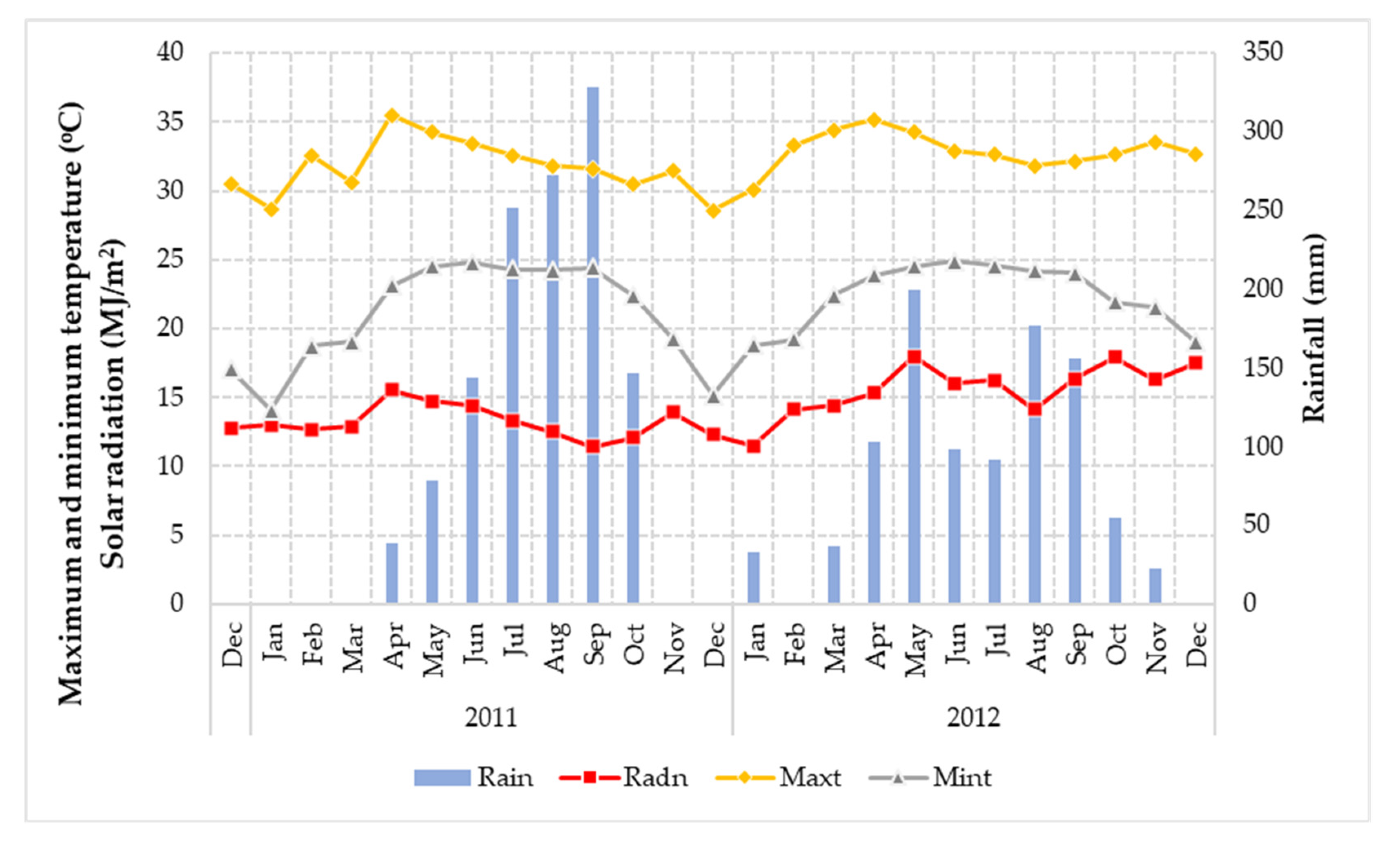
2.1. Study Field
2.2. APSIM Simulation
- sowing: from sowing to sprouting;
- sprouting: from sprouting to emergence;
- emergence: from emergence to the beginning of cane growth;
- begin cane: from the beginning of cane growth to flowering;
- flowering: from flowering to the end of the crop;
- end of the crop: crop is not currently in the simulated system.
2.3. Emulation
2.3.1. Gaussian Process-Based Emulation
2.3.2. Building Emulators
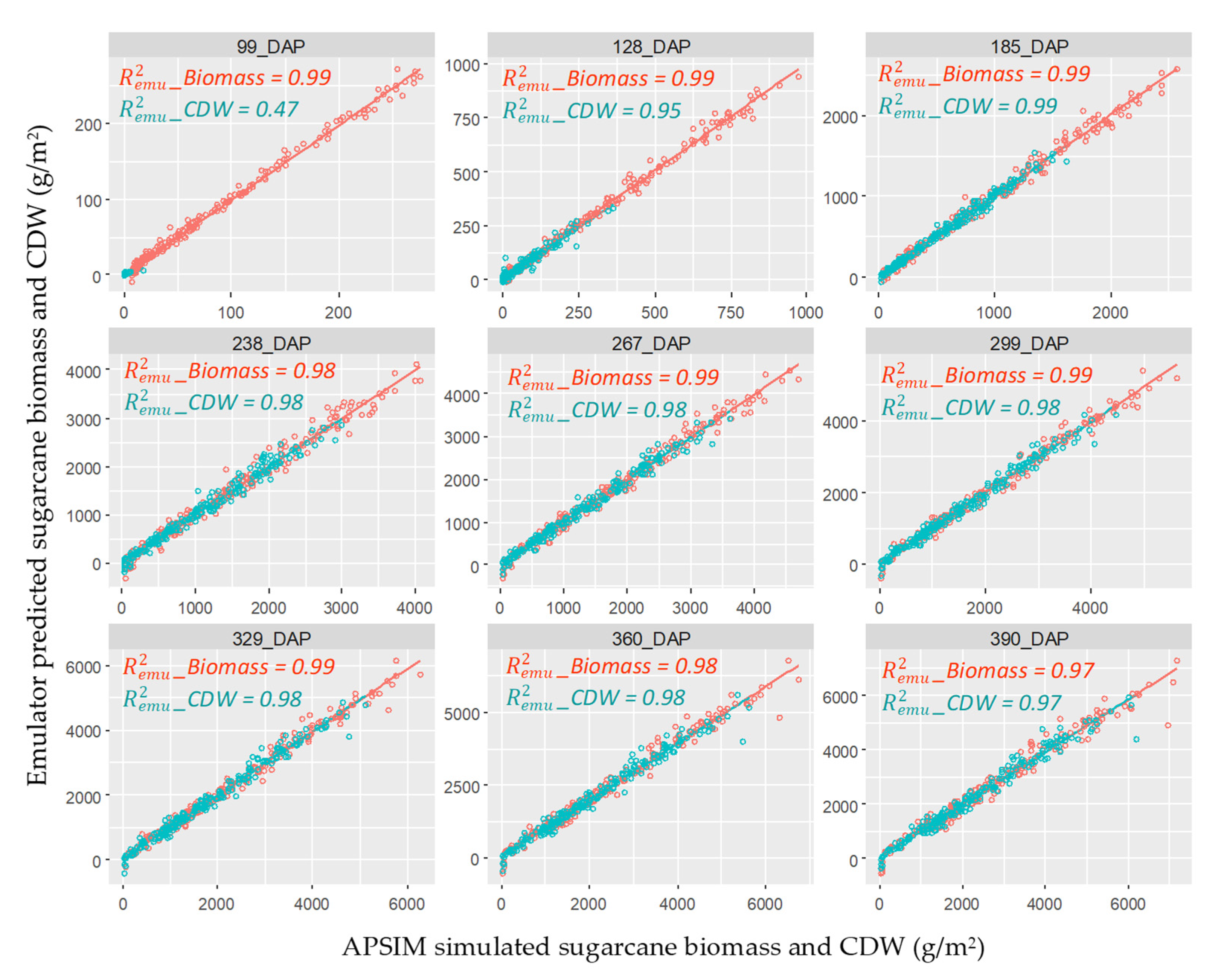
2.3.3. Emulator Accuracy Evaluation
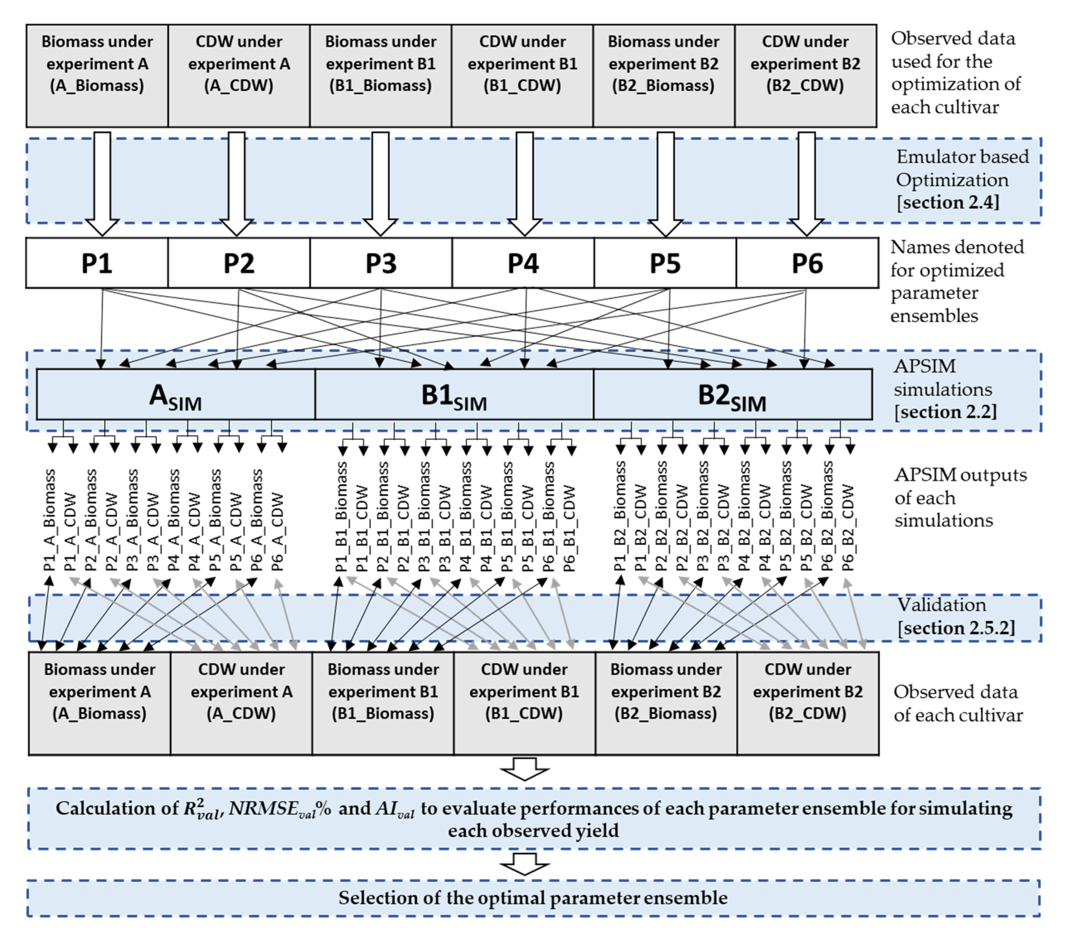
2.4. Global Optimization
2.5. Validation of Optimized Parameters
2.5.1. Validation—Step One
2.5.2. Validation—Step Two
3. Results and Discussion
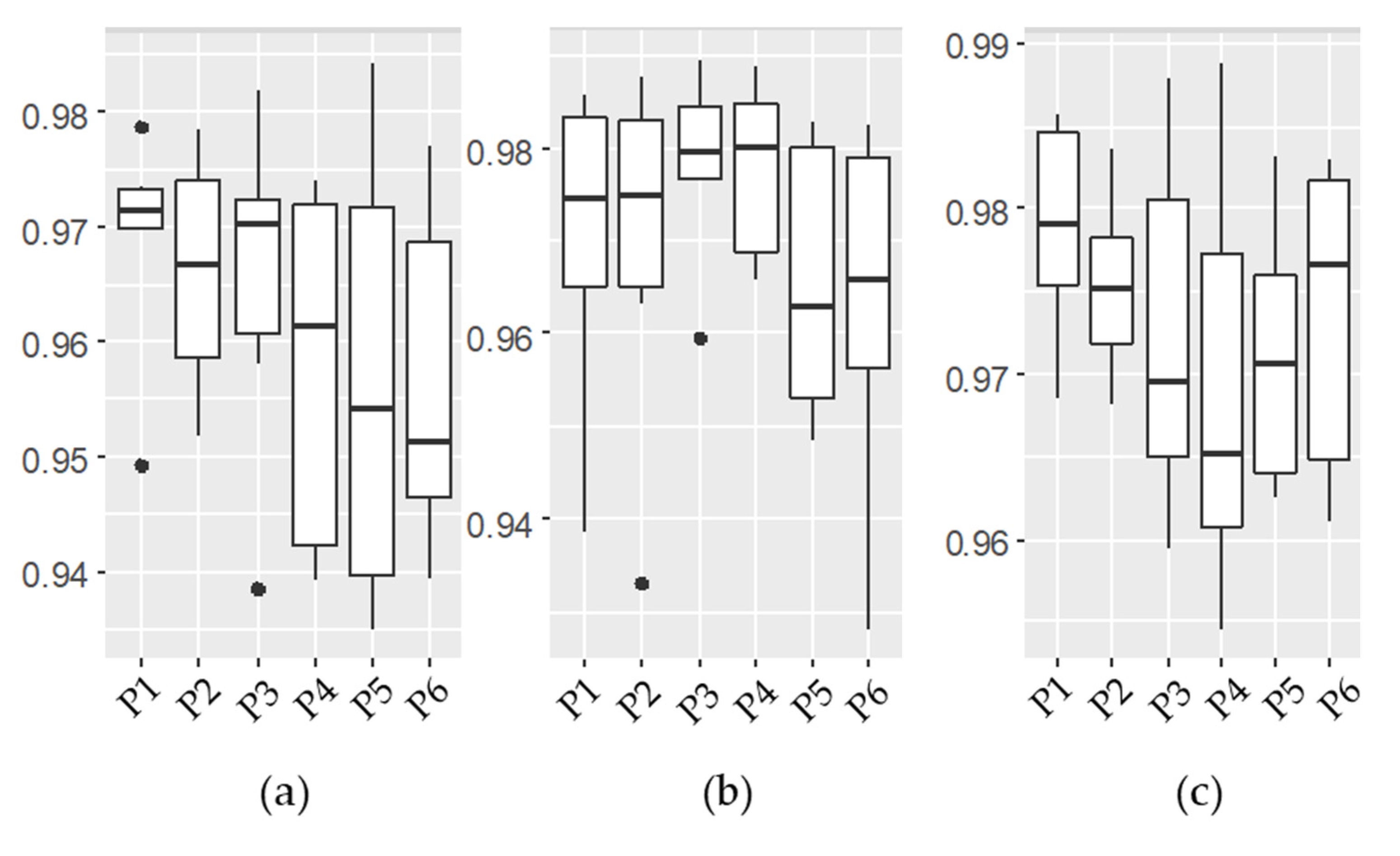
3.1. Emulator Accuracy
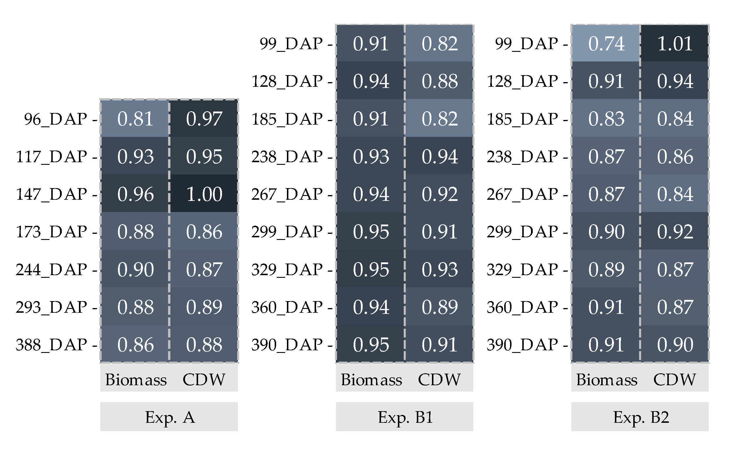
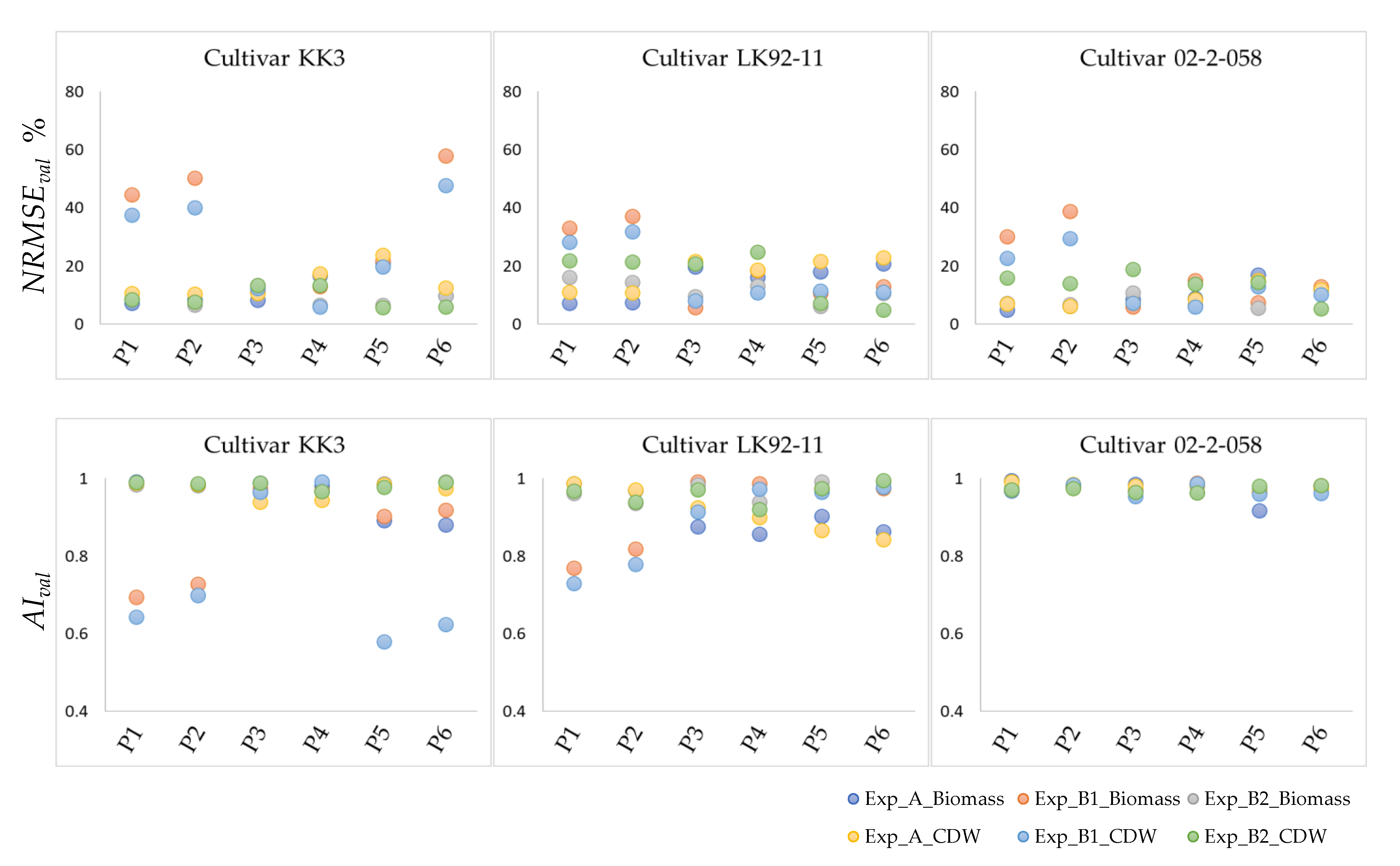
3.2. Validation of Optimized Parameters
3.2.1. Validation—Step One
3.2.2. Validation—Step Two
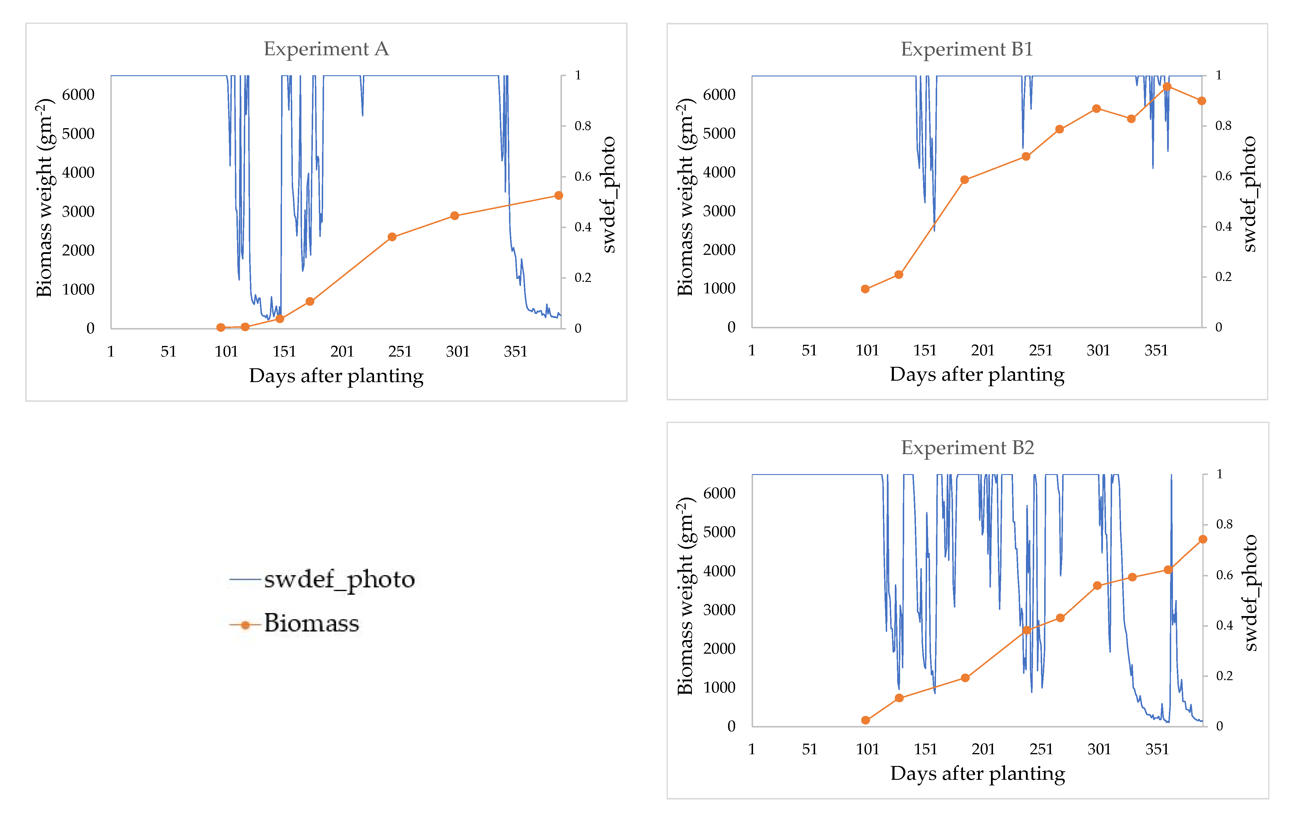
3.3. Comparison of Optimized Parameters
4. Conclusions
Supplementary Materials
Author Contributions
Funding
Data Availability Statement
Conflicts of Interest
References
- Walton, J. The 5 Countries That Produce the Most Sugar. Available online: https://www.investopedia.com/articles/investing/101615/5-countries-produce-most-sugar.asp (accessed on 2 November 2020).
- Bangkok, P. Sugar Output to Fall Short of Target Yield. Available online: https://www.bangkokpost.com/business/2136727/sugar-output-to-fall-short-of-target-yield (accessed on 27 June 2020).
- Ruan, H.; Feng, P.; Wang, B.; Xing, H.; O’Leary, G.J.; Huang, Z.; Guo, H.; Liu, D.L. Future Climate Change Projects Positive Impacts on Sugarcane Productivity in Southern China. Eur. J. Agron. 2018, 96, 108–119. [Google Scholar] [CrossRef]
- Biggs, J.S.; Thorburn, P.J.; Crimp, S.; Masters, B.; Attard, S.J. Interactions between Climate Change and Sugarcane Management Systems for Improving Water Quality Leaving Farms in the Mackay Whitsunday Region, Australia. Agric. Ecosyst. Environ. 2013, 180, 79–89. [Google Scholar] [CrossRef]
- Everingham, Y.; Inman-Bamber, G.; Sexton, J.; Stokes, C. A Dual Ensemble Agroclimate Modelling Procedure to Assess Climate Change Impacts on Sugarcane Production in Australia. Agric. Sci. 2015, 6, 870–888. [Google Scholar] [CrossRef][Green Version]
- Preecha, K.; Sakai, K.; Pisanjaroen, K.; Sansayawichai, T.; Cho, T.; Nakamura, S.; Nakandakari, T. Calibration and Validation of Two Crop Models for Estimating Sugarcane Yield in Northeast Thailand. Trop. Agric. Dev. 2016, 60, 31–39. [Google Scholar] [CrossRef]
- Sexton, J.; Inman-Bamber, N.G.; Everingham, Y.; Basnayake, J.; Lakshmanan, P.; Jackson, P. Detailed Trait Characterisation Is Needed for Simulation of Cultivar Responses to Water Stress. In Proceedings of the 36th Conference of the Australian Society of Sugar Cane Technologists, Gold Coast, Qld, Australia, 29 April–1 May 2014; pp. 82–92. [Google Scholar]
- Van Den Berg, M.; Smith, M.T. Crop Growth Models for Decision Support in the South African Sugarcane Industry. In Proceedings of the 79th Annual Congress of South African Sugar Technologists’ Association, Kwa-Shukela, Mount Edgecombe, South Africa, 19–22 July 2005; pp. 495–509. [Google Scholar]
- Keating, B.A.; Robertson, M.J.; Muchow, R.C.; Huth, N.I. Modelling Sugarcane Production Systems I. Development and Performance of the Sugarcane Module. Field Crop. Res. 1999, 61, 253–271. [Google Scholar] [CrossRef]
- Jones, M.R.; Singels, A. Refining the Canegro Model for Improved Simulation of Climate Change Impacts on Sugarcane. Eur. J. Agron. 2018, 100, 76–86. [Google Scholar] [CrossRef]
- Martiné, J.F.; Todoroff, P. Le Modèle de Croissance Mosicas et Sa Plateforme de Simulation Simulex: État Des Lieux et Perspectives. Rev. Agric. Sucrière Maurice 2002, 80, 133–147. [Google Scholar]
- Brisson, N.; Gary, C.; Justes, E.; Roche, R.; Mary, B.; Ripoche, D.; Zimmer, D.; Sierra, J.; Bertuzzi, P.; Burger, P.; et al. An Overview of the Crop Model. Stics. Eur. J. Agron. 2003, 18, 309–332. [Google Scholar] [CrossRef]
- Liu, D.L.; Bull, T.A. Simulation of Biomass and Sugar Accumulation in Sugarcane Using a Process-Based Model. Ecol. Modell. 2001, 144, 181–211. [Google Scholar] [CrossRef]
- Dias, H.B.; Inman-Bamber, G.; Everingham, Y.; Sentelhas, P.C.; Bermejo, R.; Christodoulou, D. Traits for Canopy Development and Light Interception by Twenty-Seven Brazilian Sugarcane Varieties. Field Crop. Res. 2020, 249, 107716. [Google Scholar] [CrossRef]
- Peng, T.; Fu, J.; Jiang, D.; Du, J. Simulation of the Growth Potential of Sugarcane as an Energy Crop Based on the APSIM Model. Energies 2020, 13, 2173. [Google Scholar] [CrossRef]
- Mthandi, J.; Kahimba, F.C.; Tarimo, A.K.P.R.; Salim, B.A.; Lowole, M.W. Modification, Calibration and Validation of APSIM to Suit Maize (Zea mays L.) Production System: A Case of Nkango Irrigation Scheme in Malawi. Am. J. Agric. For. 2014, 2, 1–11. [Google Scholar]
- Sun, H.; Zhang, X.; Wang, E.; Chen, S.; Shao, L.; Qin, W. Assessing the Contribution of Weather and Management to the Annual Yield Variation of Summer Maize Using APSIM in the North China Plain. Field Crop. Res. 2016, 194, 94–102. [Google Scholar] [CrossRef]
- Seidel, S.J.; Palosuo, T.; Thorburn, P.; Wallach, D. Towards Improved Calibration of Crop Models—Where Are We Now and Where Should We Go? Eur. J. Agron. 2018, 94, 25–35. [Google Scholar] [CrossRef]
- Harrison, M.T.; Roggero, P.P.; Zavattaro, L. Simple, Efficient and Robust Techniques for Automatic Multi-Objective Function Parameterisation: Case Studies of Local and Global Optimisation Using APSIM. Environ. Model. Softw. 2019, 117, 109–133. [Google Scholar] [CrossRef]
- Holzworth, D.P.; Snow, V.; Janssen, S.; Athanasiadis, I.N.; Donatelli, M.; Hoogenboom, G.; White, J.W.; Thorburn, P. Agricultural Production Systems Modelling and Software: Current Status and Future Prospects. Environ. Model. Softw. 2015, 72, 276–286. [Google Scholar] [CrossRef]
- Sheng, M.; Liu, J.; Zhu, A.X.; Rossiter, D.G.; Liu, H.; Liu, Z.; Zhu, L. Comparison of GLUE and DREAM for the Estimation of Cultivar Parameters in the APSIM-Maize Model. Agric. For. Meteorol. 2019, 278, 107659. [Google Scholar] [CrossRef]
- Sexton, J.; Everingham, Y.; Inman-Bamber, G. A Theoretical and Real-World Evaluation of Two Bayesian Techniques for the Calibration of Variety Parameters in a Sugarcane Crop Model. Environ. Model. Softw. 2016, 83, 126–142. [Google Scholar] [CrossRef]
- Georgioudakis, M.; Plevris, V. A Comparative Study of Differential Evolution Variants in Constrained Structural Optimization. Front. Built Environ. 2020, 6, 102. [Google Scholar] [CrossRef]
- Bilal; Pant, M.; Zaheer, H.; Garcia-Hernandez, L.; Abraham, A. Differential Evolution: A Review of More than Two Decades of Research. Eng. Appl. Artif. Intell. 2020, 90, 103479. [Google Scholar] [CrossRef]
- Saltelli, A.; Chan, K.; Scott, M. Sensitivity Analysis. In Probability and Statistics Series; John Wiley Sons: Chichester, UK, 2000. [Google Scholar]
- Rasmussen, C.E.; Williams, C.K.I. Gaussian Processes for Machine Learning; Dietterich, T., Bishop, C., Heckerman, D., Jordan, M., Kearns, M., Eds.; MIT Press: Cambridge, MA, USA, 2006; Volume 2, ISBN 026218253X. [Google Scholar]
- Bandara, W.B.M.A.C.; Sakai, K.; Nakandakari, T.; Kapetch, P.; Rathnappriya, R.H.K.A. Gaussian-Process-Based Global Sensitivity Analysis of Cultivar Trait Parameters in APSIM-Sugar Model: Special Reference to Environmental and Management Conditions in Thailand. Agronomy 2020, 10, 984. [Google Scholar] [CrossRef]
- Sexton, J.; Everingham, Y. Global Sensitivity Analysis of Key Parameters in A Process-Based Sugarcane Growth Model—A Bayesian Approach. In Proceedings of the 7th International Congress on Environmental Modelling and Software, San Diego, CA, USA, 15–19 June 2014. [Google Scholar]
- Sexton, J.; Everingham, Y.L.; Inman-Bamber, G. A Global Sensitivity Analysis of Cultivar Trait Parameters in a Sugarcane Growth Model for Contrasting Production Environments in Queensland, Australia. Eur. J. Agron. 2017, 88, 96–105. [Google Scholar] [CrossRef]
- Gunarathna, M.H.J.P.; Sakai, K.; Nakandakari, T.; Momii, K.; Kumari, M.K.N. Sensitivity Analysis of Plant and Cultivar-Specific Parameters of APSIM-Sugar Model: Variation between Climates and Management Conditions. Agronomy 2019, 9, 242. [Google Scholar] [CrossRef]
- Khon Kaen Climate. Available online: https://en.climate-data.org/asia/thailand/khon-kaen-province/khon-kaen-4291/ (accessed on 21 December 2020).
- USDA. Soil Texture Calculator. Available online: https://www.nrcs.usda.gov (accessed on 12 December 2020).
- Holzworth, D.; Huth, N.I.; Fainges, J.; Brown, H.; Zurcher, E.; Cichota, R.; Verrall, S.; Herrmann, N.I.; Zheng, B.; Snow, V. APSIM Next Generation: Overcoming Challenges in Modernising a Farming Systems Model. Environ. Model. Softw. 2018, 103, 43–51. [Google Scholar] [CrossRef]
- The APSIM Initiative. APSIM: The Leading Software Framework for Agricultural Systems Modelling and Simulation. Available online: https://www.apsim.info/ (accessed on 20 November 2020).
- Rohmer, J.; Foerster, E. Global Sensitivity Analysis of Large-Scale Numerical Landslide Models Based on Gaussian-Process Meta-Modeling. Comput. Geosci. 2011, 37, 917–927. [Google Scholar] [CrossRef]
- Mohammadi, H.; Challenor, P.; Goodfellow, M. Emulating Dynamic Non-Linear Simulators Using Gaussian Processes. Comput. Stat. Data Anal. 2019, 139, 178–196. [Google Scholar] [CrossRef]
- Kennedy, M.C.; O’Hagan, A. Bayesian Calibration of Computer Models. J. R. Stat. Soc. Ser. B (Stat. Methodol.) 2001, 63, 425–464. [Google Scholar] [CrossRef]
- R Core Team. R: A Language and Environment for Statistical Computing; R Foundation for Statistical Computing: Vienna, Austria, 2013; Available online: https://www.R-project.org/ (accessed on 25 November 2020).
- Ooms, J. The Jsonlite Package: A Practical and Consistent Mapping between JSON Data and R Objects. Available online: https://arxiv.org/abs/1403.2805 (accessed on 28 December 2020).
- Wickham, H.; Müller, K. Package ‘DBI.’ 2019. Available online: https://cran.r-project.org/web/packages/DBI/index.html (accessed on 24 June 2021).
- Müller, K.; Wickham, H.; James, D.A.; Falcon, S. ‘SQLite’ Interface for R. Available online: https://cran.r-project.org/web/packages/RSQLite/RSQLite.pdf (accessed on 10 December 2020).
- Kennedy, M. The GEM Software. Available online: http://www.tonyohagan.co.uk/academic/GEM/ (accessed on 23 June 2021).
- Qin, X.; Wang, H.; Li, Y.; Li, Y.; McConkey, B.; Lemke, R.; Li, C.; Brandt, K.; Gao, Q.; Wan, Y.; et al. A Long-Term Sensitivity Analysis of the Denitrification and Decomposition Model. Environ. Model. Softw. 2013, 43, 26–36. [Google Scholar] [CrossRef]
- Sexton, J. Bayesian Statistical Calibration of Variety Parameters in a Sugarcane Crop Model. Master’s Thesis, James Cook University, Townsville, Australia, April 2015. [Google Scholar]
- Kennedy, M.C.; Petropoulos, G.P. GEM-SA: The Gaussian Emulation Machine for Sensitivity Analysis. In Sensitivity Analysis in Earth Observation Modelling; George, P.P., Prashant, K.S., Eds.; Elsevier: Amsterdam, The Netherlands, 2017; pp. 341–361. ISBN 978-0-12-803011-0. [Google Scholar]
- Petropoulos, G.; Wooster, M.J.; Carlson, T.N.; Kennedy, M.C.; Scholze, M. A Global Bayesian Sensitivity Analysis of the 1d SimSphere Soil-Vegetation-Atmospheric Transfer (SVAT) Model Using Gaussian Model Emulation. Ecol. Modell. 2009, 220, 2427–2440. [Google Scholar] [CrossRef]
- Ardia, D.; Mullen, K.; Peterson, B.; Ulrich, J.; Boudt, K. Global Optimization by Differential Evolution. Available online: https://cran.r-project.org/web/packages/DEoptim/DEoptim.pdf (accessed on 28 December 2020).
- Mitchell, M. An Introduction to Genetic Algorithms, 1st ed.; MIT Press: Cambridge, UK, 1998; ISBN 0-262-13316-4. [Google Scholar]
- Oakley, J.E.; O’Hagan, A. Probabilistic Sensitivity Analysis of Complex Models: A Bayesian Approach. J. R. Stat. Soc. Ser. B Stat. Methodol. 2004, 66, 751–769. [Google Scholar] [CrossRef]
- Kennedy, M.C.; O’Hagan, A.; Higgins, N. Bayesian Analysis of Computer Code Outputs. In Quantitative Methods for Current Environmental Issues; Anderson, C.W., Barnett, V., Chatwin, P.C., El-Shaarawi, A.H., Eds.; Springer: London, UK, 2004; pp. 227–243. ISBN 978-1-4471-0657-9. [Google Scholar]
- Singels, A.; Bezuidenhout, C.N. A New Method of Simulating Dry Matter Partitioning in the CANEGRO Sugarcane Model. Field Crop. Res. 2002, 78, 151–164. [Google Scholar] [CrossRef]
- Peerasak, S. Evaluation of Elite Sugarcane Clones Suitable for Growing Areas. In Progress Report under Project Develop and Engineering No. 7; J-STAGE: Japan, 2013; p. 174. [Google Scholar]
- Cha-um, S.; Wangmoon, S.; Mongkolsiriwatana, C.; Ashraf, M.; Kirdmanee, C. Evaluating Sugarcane (Saccharum sp.) Cultivars for Water Deficit Tolerance Using Some Key Physiological Markers. Plant Biotechnol. 2012, 29, 431–439. [Google Scholar] [CrossRef]
- Khonghinta, J.; Khruengpat, J.; Songsri, P.; Gonkhamdee, S.; Jongrungkl, N. Classification of the Sugar Accumulation Patterns in Diverse Sugarcane Cultivars under Rain-Fed Conditions in a Tropical Area. J. Agron. 2020, 19, 94–105. [Google Scholar] [CrossRef][Green Version]


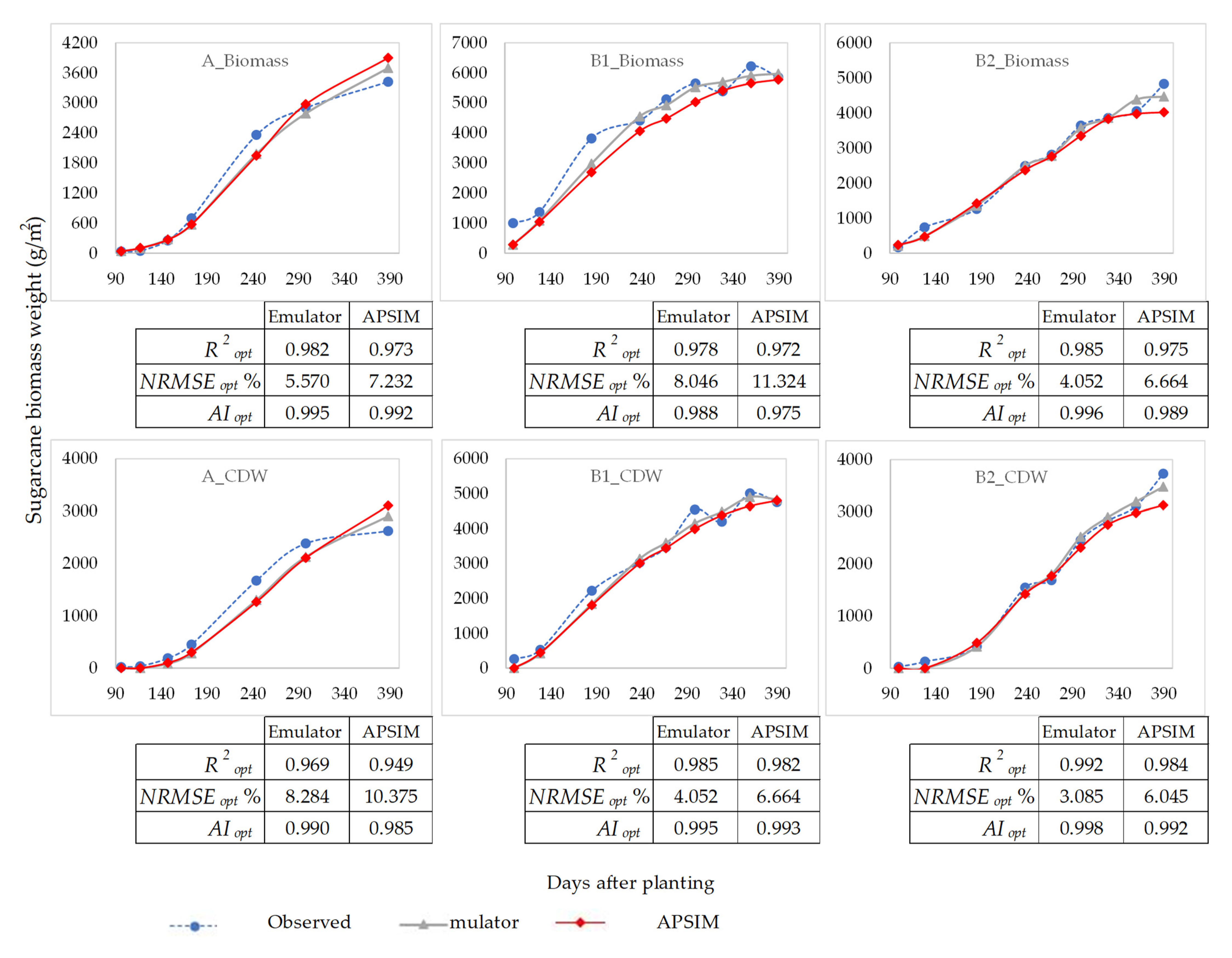
 : Biomass and
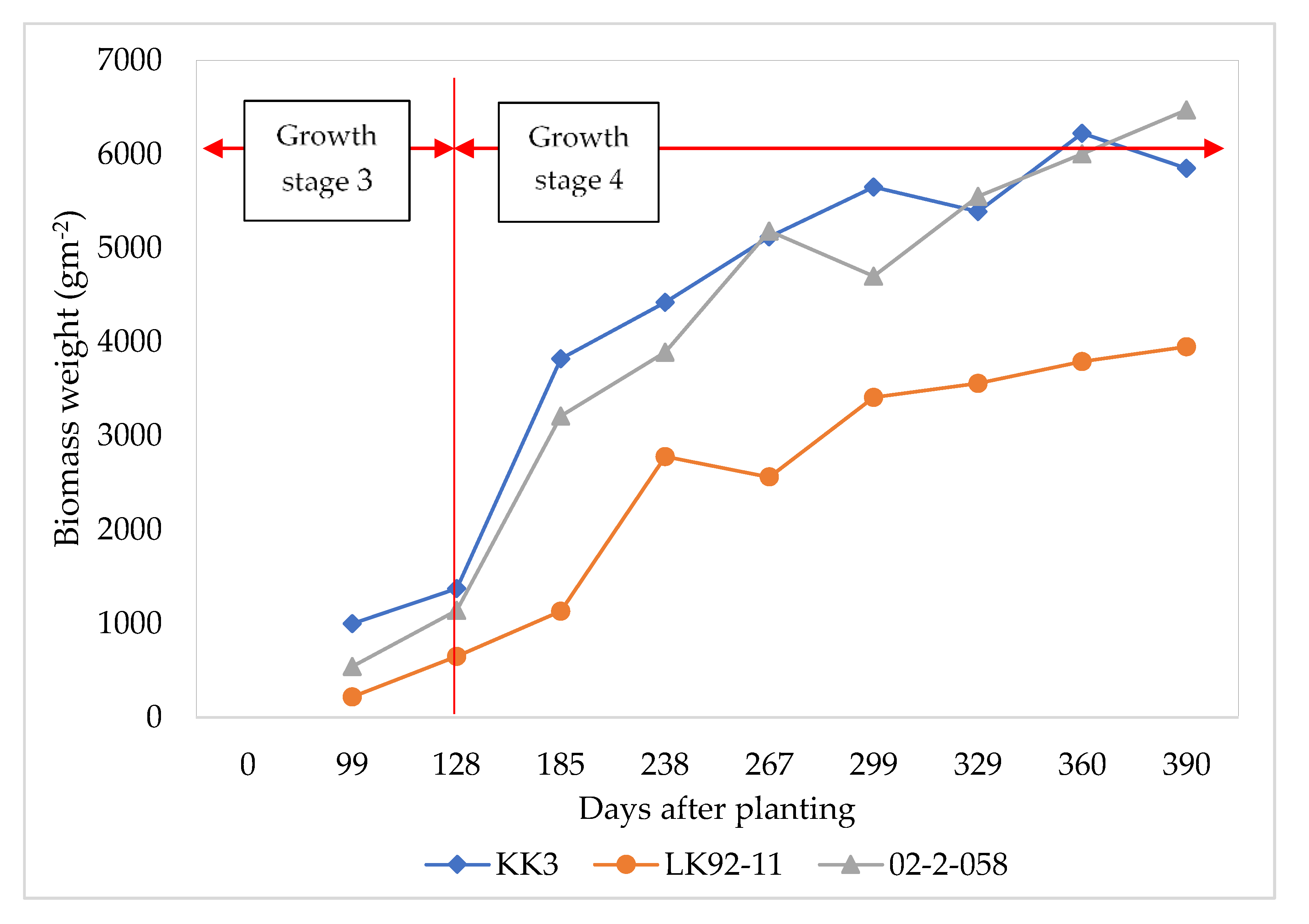
  : CDW. _Biomass and CDW were calculated by using 200 data points.
: Biomass and : CDW. _Biomass and CDW were calculated by using 200 data points.
: CDW. _Biomass and CDW were calculated by using 200 data points.
: Biomass and : CDW. _Biomass and CDW were calculated by using 200 data points.


| Experiment A | Experiments B1 and B2 | |
|---|---|---|
| Planting date | 1/12/2010 | 28/11/2011 |
| Harvesting date | 20/12/2011 | 22/12/2012 |
| Cultivars | 02-2-058, KK3, LK92-11 | |
| Water supply | Rainfed a (A) | Irrigated b (B1) and Rainfed a (B2) |
| Fertilizer | 93.5:40.80:77.62 kg of N:P:K per hectare | |
| Observed data | Biomass and CDW of experiment A were recorded at; 96, 117, 147 173, 244, 29 and 388 days after planting (DAP) and experiment B1 and B2 at; 99, 128, 185, 238, 267, 299, 329, 360 and 390 DAP | |
| Soil Depth (cm) | Texture Class * | Wilting Point (mm/mm) | Field Capacity (mm/mm) | Saturation (mm/mm) | Hydraulic Conductivity (mm/day) | Bulk Density (g/cm3) |
|---|---|---|---|---|---|---|
| 0–20 | Loamy soil | 0.075 | 0.206 | 0.357 | 3336 | 1.52 |
| 20–50 | Sandy loam | 0.116 | 0.236 | 0.395 | 2232 | 1.61 |
| 50–100 | Sandy clay loam | 0.124 | 0.238 | 0.410 | 2232 | 1.57 |
| Function of Parameters | Parameter Name | Description | Level | Code | Units | Parameter Space * |
|---|---|---|---|---|---|---|
| Canopy development | leaf_size | Area of the respective leaf | leaf_size_no = 1 | LS1 | mm2 | 500–2000 |
| leaf_size_no = 14 | LS2 | mm2 | 20,000–70,000 | |||
| leaf_size_no = 20 | LS3 | mm2 | 20,000–70,000 | |||
| green_leaf_no | Maximum number of fully expanded green leaves | GLN | No. | 9–15 | ||
| tillerf_leaf_size | Tillering factors according to the leaf numbers | Tiller_leaf_size_no = 1 | TLS1 | mm2/mm2 | 1–6 | |
| Tiller_leaf_size_no = 4 | TLS2 | mm2/mm2 | 1–6 | |||
| Tiller_leaf_size_no = 10 | TLS3 | mm2/mm2 | 1–6 | |||
| Tiller_leaf_size_no = 16 | TLS4 | mm2/mm2 | 1–6 | |||
| Tiller_leaf_size_no = 26 | TLS5 | mm2/mm2 | 1–6 | |||
| Partitioning of assimilates | cane_fraction | Fraction of accumulated biomass partitioned to cane | CF | g/g | 0.65–0.80 | |
| sucrose_fraction_stalk | Fraction of accumulated biomass partitioned to sucrose | SF1 | g/g | 0.40–0.70 | ||
| stress_factor_stalk | Stress factor for sucrose accumulation | SF2 | n/a | 0.2–1.0 | ||
| sucrose_delay | Sucrose accumulation delay | SD | g/m2 | 0–600 | ||
| min_sstem_sucrose | Minimum stem biomass before partitioning to sucrose commences | MSS | g/m2 | 400–1500 | ||
| Phenological development based on thermal time | min_sstem_sucrose_redn | Reduction to minimum stem sucrose under stress | MSSR | g/m2 | 0–20 | |
| tt_emerg_to_begcane | Accumulated thermal time from emergence to beginning of cane | EB | °C day | 1200–1900 | ||
| tt_begcane_to_flowering | Accumulated thermal time from beginning of cane to flowering | BF | °C day | 5400–6600 | ||
| tt_flowering_to_crop_end | Accumulated thermal time from flowering to end of the crop | FC | °C day | 1750–2250 | ||
| Dry matter assimilation | transp_eff_cf | Transpiration efficiency coefficient | From sowing to sprouting | TEC1 | kg kPa/kg | 0.006–0.014 |
| From sprouting to emergence | TEC2 | |||||
| From emergence to the beginning of cane growth | TEC3 | |||||
| From the beginning of cane growth to flowering | TEC4 | |||||
| From flowering to the end of the crop | TEC5 | |||||
| At the end of the crop | TEC6 | |||||
| rue | Radiation use efficiency | From emergence to the beginning of cane growth | RUE3 | g/MJ | 0.74–2.5 | |
| From the beginning of cane growth to flowering | RUE4 | |||||
| From flowering to the end of the crop | RUE5 |
| Parameter Name | Code | Unit | Cultivar | ||
|---|---|---|---|---|---|
| KK3 (P3) | LK92-11 (P5) | 02-2-058 (P3) | |||
| leaf_size | LS1 | mm2 | 1566 | 1792 | 1790 |
| LS2 | 62,686 | 56,809 | 20,252 | ||
| LS3 | 47,681 | 68,364 | 61,664 | ||
| cane_fraction | CF | g/g | 0.65 | 0.66 | 0.68 |
| sucrose_fraction_stalk | SF1 | g/g | 0.7 | 0.6 | 0.5 |
| stress_factor_stalk | SF2 | n/a | 0.9 | 0.9 | 0.9 |
| sucrose_delay | SD | g/m2 | 582 | 563 | 137 |
| min_sstem_sucrose | MSS | g/m2 | 432 | 1097 | 1420 |
| min_sstem_sucrose_redn | MSSR | g/m2 | 19 | 0.26 | 2 |
| tt_emerg_to_begcane | EB | °C day | 1537 | 1874 | 1397 |
| tt_begcane_to_flowering | BF | °C day | 5404 | 5748 | 6523 |
| tt_flowering_to_crop_end | FC | °C day | 2138 | 2153 | 1794 |
| green_leaf_no | GLN | No. | 14 | 15 | 14 |
| tillerf_leaf_size | TLS1 | mm2/mm2 | 5 | 4 | 3 |
| TLS2 | 3 | 4 | 3 | ||
| TLS3 | 1 | 1 | 1 | ||
| TLS4 | 4 | 5 | 3 | ||
| TLS5 | 3 | 3 | 5 | ||
| transp_eff_cf | TEC1 | kg kPa/kg | 0.008 | 0.014 | 0.010 |
| TEC2 | 0.007 | 0.014 | 0.011 | ||
| TEC3 | 0.013 | 0.013 | 0.012 | ||
| TEC4 | 0.014 | 0.009 | 0.014 | ||
| TEC5 | 0.014 | 0.013 | 0.013 | ||
| TEC6 | 0.011 | 0.014 | 0.010 | ||
| rue | RUE3 | g/MJ | 2.50 | 2.24 | 2.49 |
| RUE4 | 2.46 | 2.34 | 2.48 | ||
| RUE5 | 1.14 | 2.40 | 1.84 | ||
Publisher’s Note: MDPI stays neutral with regard to jurisdictional claims in published maps and institutional affiliations. |
© 2021 by the authors. Licensee MDPI, Basel, Switzerland. This article is an open access article distributed under the terms and conditions of the Creative Commons Attribution (CC BY) license (https://creativecommons.org/licenses/by/4.0/).
Share and Cite
Bandara, W.B.M.A.C.; Sakai, K.; Nakandakari, T.; Kapetch, P.; Anan, M.; Nakamura, S.; Setouchi, H.; Rathnappriya, R.H.K. Global Optimization of Cultivar Trait Parameters in the Simulation of Sugarcane Phenology Using Gaussian Process Emulation. Agronomy 2021, 11, 1379. https://doi.org/10.3390/agronomy11071379
Bandara WBMAC, Sakai K, Nakandakari T, Kapetch P, Anan M, Nakamura S, Setouchi H, Rathnappriya RHK. Global Optimization of Cultivar Trait Parameters in the Simulation of Sugarcane Phenology Using Gaussian Process Emulation. Agronomy. 2021; 11(7):1379. https://doi.org/10.3390/agronomy11071379
Chicago/Turabian StyleBandara, W. B. M. A. C., Kazuhito Sakai, Tamotsu Nakandakari, Preecha Kapetch, Mitsumasa Anan, Shinya Nakamura, Hideki Setouchi, and R. H. K. Rathnappriya. 2021. "Global Optimization of Cultivar Trait Parameters in the Simulation of Sugarcane Phenology Using Gaussian Process Emulation" Agronomy 11, no. 7: 1379. https://doi.org/10.3390/agronomy11071379
APA StyleBandara, W. B. M. A. C., Sakai, K., Nakandakari, T., Kapetch, P., Anan, M., Nakamura, S., Setouchi, H., & Rathnappriya, R. H. K. (2021). Global Optimization of Cultivar Trait Parameters in the Simulation of Sugarcane Phenology Using Gaussian Process Emulation. Agronomy, 11(7), 1379. https://doi.org/10.3390/agronomy11071379