Abstract
Climate change calls for novel approaches to include environmental effects in future breeding programs for forage crops. A set of ryegrasses (Lolium) varieties was evaluated in multiple European environments for crown rust (Puccinia coronata f. sp. lolii) and stem rust (P. graminis f. sp. graminicola) resistance. Additive Main Effect and Multiplicative Interaction (AMMI) analysis revealed significant genotype (G) and environment (E) effects as well as the interaction of both factors (G × E). Genotypes plus Genotype-by-Environment interaction (GGE) analysis grouped the tested environments in multiple mega-environments for both traits suggesting the presence of an environmental effect on the ryegrasses performances. The best performing varieties in the given mega-environments showed high resistance to crown as well as stem rust, and overall, tetraploid varieties performed better than diploid. Furthermore, we modeled G × E using a marker x environment interaction (M × E) model to predict the performance of varieties tested in some years but not in others. Our results showed that despite the limited number of varieties, the high number of observations allowed us to predict both traits’ performances with high accuracy. The results showed that genomic prediction using multi environmental trials could enhance breeding programs for the crown and stem rust in ryegrasses.
1. Introduction
Perennial ryegrass (Lolium perenne L.), as well as Italian ryegrass (Lolium multiflorum Lam.), are extensively used in temperate regions as a forage crop and as turf for recreational areas.
Foliar diseases of ryegrasses caused by fungi belonging to the genus Puccinia are the most damaging, causing a reduction in tillering, root and shoot biomass, and plant regrowth [1]. Consequently, the infection reduces the quality of pastures used for meat, milk, and wool production and damages turf used for recreation [2]. The two most common rust diseases in ryegrasses are crown rust, caused by Puccinia coronata f. sp. lolii, and stem rust, caused by P. graminis f. sp. graminicola [3,4,5].
Crown rust disease appears on ryegrasses in summer after the release of urediniospores, which can re-infect ryegrass plants and produce a more robust infection. Due to the asexual reproduction cycle of crown rust on the primary host, multiple ryegrass plants’ infections occur within one growing season. In autumn, the teliospores’ germination leads to basidiospores’ formation, which, carried by the wind, moves to the alternative host, common buckthorn (Rhamnus cathartica L.), where the sexual reproduction may occur.
Stem rust affects mainly seed production in perennial ryegrass, causing a seed yield reduction [6]. Sexual reproduction often occurs on the alternative host barberry (Berberis vulgaris L.). Considering both rust species’ destructive potential, crown and stem rust resistance are essential in variety registration and are fundamental goals in ryegrass breeding [7].
The sexual phase of crown and stem rust contributes to the increase of genetic variability in the pathogen population [8]. Indeed, the eradication of the alternative host of stem rust in the United States revealed a large impact on reducing genetic diversity [8]. Nevertheless, variability in the virulence of crown rust populations in the absence of the sexual stage exists due to other factors, such as high mutation rates or somatic hybridization and recombination [9]. Genetic variability leads to the presence of multiple pathotypes that might show diverse levels of virulence in the host population.
Phenotypic diversity can also be observed in plants subjected to various environments; variability in response derives from the environment’s effect on the expression and function of genes associated with the trait of interest. Environmental conditions such as temperature, light, and dew might influence the infection process, as previously reported for the penetration rate of crown and stem rust in oats [10] and wheat stem rust epidemics [11].
The analysis of genotype-by-environment interaction (GEI) in Multi Environmental Trials (METs) is commonly conducted in breeding programs to select superior genotypes across different locations, collecting information about the environmental effects, as well as for predicting the performance of untested genotypes. Understanding the host-by-pathogen interaction patterns can be challenging due to the genetic variability of both the host and the pathogen and the effect of the environment; therefore, the identification of stable and durable resistance varieties of ryegrasses against crown and stem rust is desired.
Several studies have been conducted to evaluate the level of genotypic stability in MET experiments confirming the role of GEI in the response variability of the tested performers [12,13,14,15,16]. Understanding the role of GEI on the pathosystem and host stability across multi environments is essential for a successful breeding program. Multi environment testing is extensively used to analyze the adaptability and stability of varieties to diseases and investigate the GEI effect on important agronomic traits [17,18,19,20]. The most frequently used approaches for characterizing GEI effects are Additive Main Effect and Multiplicative Interaction (AMMI) analysis and site regression of Genotypes (G) plus Genotype-by-Environment (GE) interaction (GGE) biplot analysis. Both AMMI [21] and GGE biplot [22] methods combine the principal component analysis (PCA) with the ANOVA method into a single analysis. The main difference between these two methods is the initial analysis where GGE models G+GE directly, while the AMMI model separates G from GE. Due to the portioning of the phenotypic variation into genotype main effect, environment main effect, and genotype-by-environment interaction, the AMMI model is considered superior to linear regression [23]. On the other hand, GGE biplot analysis is deemed useful to determine the best performer for a group of environments (mega-environment) by identifying the most tolerant and stable varieties [24]. Since a mega-environment identified with GGE analysis is defined as a group of locations that share the best set of varieties over the years [25], data from several years are required to determine whether or not the target area can be separated into different mega-environments. The detection of mega-environments is correlated with the recognition of GEI patterns across different locations, and its investigation is essential for cultivar evaluation and recommendation [26]. An advantage of these two approaches is the graphical interpretation of the statistical analysis results using a biplot, which contains information of both genotypes and environments.
The availability of dense marker sets made it possible to implement genomic selection (GS) in plant breeding [27]. Numerous studies have demonstrated the benefit of including marker information in GEI programs, leading to increased prediction accuracy [28,29,30,31]. Several GS studies have been conducted to predict varieties performances in METs by using covariance functions [28], markers, and environmental covariates [32] or by modeling marker x environment (M × E) interactions [33]. The M × E approach has been extended to whole-genome regression models by Lopez-Cruz et al. [30], where phenotypes were regressed on a large number of genome-wide markers. This approach has been extensively used in several investigations showing that modeling M × E interactions can improve the prediction accuracy [28,29,31,34,35]. In the M × E model, marker effects are decomposed into components that are stable across environments (main effect) and environment-specific deviations (interactions).
Genomic prediction has been applied to several traits in ryegrasses, such as heading date, seed yield, dry matter yield, neutral detergent fiber, fructan as well as crown rust resistance [36,37,38,39].
In this investigation, phenotypic data collected between 2001 and 2013 from 34 locations, as part of the EUCARPIA multi-site rust evaluation trial [4,40], were used to study the environment’s role in driving the plant-pathogen interaction.
The main goals of this study were (i) to evaluate the GEI using AMMI and GGE analysis for crown and stem rust resistance in multi environmental trials in ryegrasses, and (ii) to apply the M × E model of Lopez-Cruz et al. [30] for genomic prediction of crown and stem rust in a high dense MET.
2. Materials and Methods
2.1. Experimental Data and Phenotypic Analysis
Crown and stem rust resistance were tested on a set of 34 perennial (L. perenne), 16 Italian (L. multiflorum), and 4 hybrid (L. boucheanum) ryegrasses. The field trials were conducted as described by Schubiger and Boller [4,40] in 34 locations across Europe (Table S1; Figure 1). The experiments were performed every three years from 2001 to 2013 in a randomized complete block design with four replications. The varieties were sown as rows of 3 m length and with 0.5 m spacing. Rust incidence based on natural infection was scored visually on a scale from 1 to 9, with 1 meaning no rust disease and 9 more than 75% of the foliage covered by rust-affected leaf area (Table S2). The rating values reported a relative estimation of the leaf area occupied by rust pustules and chlorosis or necrosis, as described by Schubiger et al. [4]. For better visualization of the data, in this investigation, the scale was inverted so that lower values refer to a lower tolerance level (higher susceptibility) and higher scores to a higher tolerance to the rust infection. Furthermore, for the statistical analysis, the collected observations were divided into four groups: PCO-LP, PCO-LM, PGR-LP, and PGR-LM, including data from testing crown rust (PCO) and stem rust (PGR) resistance on perennial ryegrass (LP) and Italian and hybrid ryegrass (LM) varieties, respectively.
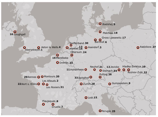
Figure 1.
Geographical position of the experimental sites. Numbers close to location names refer to the site numbers used during the analysis.
Dispersion of crown and stem rust scorings across the years of the trials were analyzed by computing the coefficient of variation (CVar). Trait repeatability [41] as estimation of genetic influence on the trait was calculated as σ2g/(σ2g + σ2e), where σ2g stands for total genetic variance and σ2e the residual variance.
2.2. AMMI and GGE Analysis of Crown and Stem Rust
Adaptability and genotype stability in the different locations were estimated by the AMMI (1) and GGE (2) models:
where is the mean response of the variety ith in the environment jth; is the overall mean of the test; is the genotypic effect; is the site effect; is the number of SVD (singular value decomposition) axes retained in the model, (λ1 ≥ λ2 ≥ … ≥ λt) are the singular values for SVD axis , = (, …, ) are the genotype singular vector values for SVD axis , = (, …, ) are the environment singular vector values for SVD axis , is the residual term.
Analysis of variance for PGR and PCO was performed separately for perennial and Italian ryegrass, where environments refer to a combination of location and year.
Interaction Principal Component Axis (IPCA) analysis was used to portion the sum of squares (SS) into different AMMI models. The F-test of Gollob [42] was used to select the model that best describes the G × E interaction by evaluating the significance of each IPCA (Factors) related to the mean square (MS) error of the axes to be retained in the model [21]. The AMMI and GGE results were graphically visualized on a biplot to identify the most resistant and stable varieties in different environments, as well as to explore the presence of multiple mega-environments with unique best performers. The GEA-R (Genotype × Environment Analysis with R) program developed by Pacheco et al. [43] was used to perform the AMMI and GGE analysis.
Pearson’s rank correlation coefficients were calculated among the ranks given by the different statistical methods. The AMMI analysis ranks were obtained by assigning the highest level to the variety with the smallest AMMI stability value (ASV), which refers to the distance from the biplot origin reporting IPCA1 scores against IPCA2 scores. The ASV was calculated with the following formula, as previously described by Purchase et al. [44]:
where is the weight derived from dividing the sum of squares by the sum of squares. AMMI stability analysis was conducted using the R function index. AMMI in the package agricolae [45].
2.3. Genotyping
For each variety, DNA was isolated from leaves of 0.5 g germinated seedlings, according to Byrne et al. [46]. Sequence data were produced by Genotyping-By-Sequencing (GBS) according to Elshire et al. [47] using the restriction enzyme ApeKI for complexity reduction. A single GBS library was prepared for the 54 varieties and sequenced on a single Illumina HiSeq4000 lane as 100 bp single-end. After basic data filtering and de-multiplexing using Sickle [48] and Sabre (github.com/najoshi/sabre), respectively, reads were aligned to a perennial ryegrass pseudo-chromosome assembly (Nagy et al., 2021;- manuscript in preparation) using BWA [49]. Variant calling was performed using GATK’s HaplotypeCaller and CombineGVCFs [50], and SelectVariants was used to filter for biallelic sites and mapping quality (MQ) of 30. Vcftools [51] was used to filter the data for max missing per site (20%) and a minor allele frequency (0.02).
2.4. Genomic Prediction of Crown and Stem Rust Resistance
Following Lopez-Cruz et al. [30], an interaction model was considered to predict the varieties genetic values in the four datasets (PCO-LP, PCO-LM, PGR-LP, and PGR-LM). Only locations tested for a minimum of three years were included for the genomic prediction analysis. In the M × E model, the kth marker effect in the jth environment (βjk) is modeled as the sum of the main effect (bok) plus an interaction term bjk representing a deviation from the main effect unique to the jth environment (βjk = bok + bjk). The model can be described as:
where is an intercept, represents the main effect with ~ N(0,Gσ²b0k), explain the interaction effect with ~ N(0,Gσ²bjk), is the vector of model residuals ~ N(0,1), where G is the relationship matrix of marker-centered and standardized genotypes.
The model was implemented using the Bayesian Generalized Linear Regression (BGLR) R package [52]. For the estimation of the variance components, the model was fitted to data from each environment separately, and for each data set, the magnitude of main and interaction effect was determined by the estimation of variance components. Settings in the model for estimating the fixed effect, markers’ main effect, and interaction terms were set as default, as shown by Lopez-Cruz et al. [30]. Following Burgueño et al. [28], the cross-validation (CV) considered during the analysis represented the scenario of having an incomplete field trial (CV2). Through that, performances of varieties were predicted in environments in which they have not been evaluated. Training and testing (TRN-TST) partitions for CV2 were generated as described by Roorkiwal et al. [53]. The phenotypes were randomly split into five subsets, with 80% of the lines assigned to the training set and 20% to the testing set. The training set was composed of four subsets, with the remaining subset serving as the validation set, which led to five possible TRN-TST sets. The cross-validation was repeated 25 times. For each TRN-TST set, the M × E model was fitted to the TRN data set, and prediction accuracy was assessed by computing the Brier score [54], which is equal to:
where is the probability of the predictive distribution, takes a value of 1 if the categorical response observed for individual falls into category , and 0 otherwise. We reported the average Brier score and standard deviation from 25 subsequent iterations.
3. Results
3.1. Phenotypic Analysis of Crown and Stem Rust Disease
The range of values in both crown and stem rust scorings showed a similar dispersion around the mean, as described by the coefficient of variation (CVar), which was on average 31.62 for PCO and 24.91% for PGR, with the year 2010, showing a lower CVar compared to the others (Table 1 and Table 2). This result indicates that the virulence of both crown and stem rust species in Europe did not change significantly during the period of the experiment. Confirmation of the absence of virulence variations was obtained by PGR and PCO’s trait repeatability within years that did not change from 2001 to 2013, except for 2010 (0.52) and 2013 (0.15), which showed the highest and lowest values for PGR, respectively. These exceptions are probably due to the significantly reduced number of observations (624) in 2010 compared to the other years (1530, on average) and the high CVar of 2013 (32.74) given the low number of records (1488). Both LP and LM showed more resistance to PGR infection, as indicated by the mean scores of 6.4 (LP) and 6.9 (LM), compared to PCO infection, 5.8 (LP) and 5.9 (LM).

Table 1.
Crown rust (PCO) phenotypic distribution per year. The number of observations (n), lowest (min), highest (max) and mean score per year; standard deviation (Sd); coefficient of variation (CVar) calculated as Sd*100/mean; trait repeatability estimates.
Table 2.
Stem rust (PGR) phenotypic distribution per year. The number of observations (n), lowest (min), highest (max) and mean score per year; standard deviation (Sd); coefficient of variation (CVar) calculated as Sd*100/mean; trait repeatability estimates.
3.2. Genotypic Analysis
A total of 2,870,878,736 reads were obtained from the sequencing, with 98.02% of nucleotides showing a quality value larger than 20 (Q20). After filtering the markers, a total of 686,960 SNPs were used for subsequent analysis. The population structure study revealed a clear stratification among the 54 varieties based on the species (principal component 1) and the ploidy (principal component 2) (Figure 2).
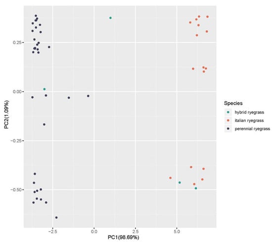
Figure 2.
Principal component analysis (PCA) showing the population structure of the 54 varieties based on the 686,960 SNP markers. The colors refer to the three species: blue for perennial ryegrass, orange for Italian ryegrass and green for hybrid ryegrass.
The narrow-sense heritability estimates for crown and brown rust resistance across all years and locations were 0.29 and 0.06, respectively.
3.3. AMMI Analysis of Crown and Stem Rust Resistance
The combined ANOVA and AMMI analysis for PCO and PGR analysis indicated highly significant differences (p ≤ 0.001) for the genotype, environment, and G × E interaction terms (Table 3). In PGR-LP, the genotype (G) and environment (E) explained 41.7% and 43.7% of the variation, respectively, and 21.8% and 58.5% for PGR-LM. For PCO, G and E explained 36.6% and 45.2% in LP and 63.1% and 24.7% in LM. GE interaction explained 14.6% and 19.6% of the variation in PGR-LP and PGR-LM, respectively, and 12.2% and 18.2% for PCO-LM and PCO-LP. Using the AMMI model to partition the GE interaction effects showed that the first two interaction principal components (IPCA1 and IPCA2) significantly and cumulatively captured 49.5% (PGR-LP), 69.6% (PGR-LM), 48.5% (PCO-LP), and 63.3% (PCO-LM) of the G × E interaction (Table 3).
Table 3.
AMMI analysis for PGR (a) and PCO (b); analysis of variance for the significant effect of genotype (variety) (G), environment (E), genotype-by-environment interaction (GEI). Degrees of freedoms (Df); sum of square (SS); percentage of variance explained (%); mean of square (MS); F test of Gollub (F); residual (Res); statistical significance code: ** p ≤ 0.01, *** p ≤ 0.001. (A) PGR and (B) PCO. Partitioning of GEI into AMMI axes PC1, PC2 and PC3.
Environmental effect on the variety’s performances can be observed in the AMMI1 biplot by showing the variation of the overall rust mean on the abscissa and IPCA1 values on the ordinates (Figure 3). The lower the IPCA1, the lower the GEI effect and the higher the variety’s stability. The genotypes that contributed most to the GE interaction in PGR-LP (Figure 3a) were Maja, Aurora, and Fennema, and those who contributed the least being the most stable, were Guru, Gladio, Aristo, Carrera, Lacerta, Orval, Aubisque, Bocage and Gwendal. Of these, the variety Bocage and Gwendal had the highest PGR scores, exceeding the overall mean. For PGR-LM (Figure 3b), varieties Crema, Barprisma, Fastyl, Tarandus, and Domino are the most stable since the coordinates on the axis were the lowest IPCA1, with the last two varieties having a mean resistance score higher than the overall mean. In PCO-LP (Figure 3c), varieties Aberdart, Roy, Orval, and Pastoral had high stability and resistance values close to the mean, while Lacerta, Bocage, and Gwendal had the highest PCO resistance scores and moderate stability. Varieties Condensa and Vincent are the ones with the highest GE effect. In the PCO-LM set (Figure 3d), varieties Meryl, Pirol (LB), Aberexcel, Caballo, and Domino had the highest stability across environments, and the last three varieties had higher values than the mean.
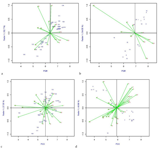
Figure 3.
AMMI 1 biplot of IPCA1 vs PGR-LP mean (a), PGR-LM mean (b), PCO-LP (c), and PCO-LM (d). The blue numbers represent ryegrass varieties, whereas the red numbers indicate the environments. The green arrows indicate the environmental vectors. The arrows’ length indicates the variability in the varieties’ response to that particular environment: the longer the arrow, the higher is the response variability.
Details about the severity of the infection at the tested location and the variability in the response of the tested varieties can be seen in Figure 3. In Radzików (Poland), Orchies (France) and Steinach (Germany), LP varieties showed high response variability and susceptibility to PGR, while LM varieties performed worst in Orchies (France), Hladke Zivotice (Czechia) and Les Rosiers (France). On the other hand, high levels of tolerance and more response stability were detected in LP varieties in Malchow (Germany), Montours (France) and Spitalhof (Germany) and by evaluating LM varieties in Lodi (Italy), Gumpenstein (Austria) and Steinach (Germany). Higher levels of variability and susceptibility to PCO were detected testing LP in Nort s. E. (France), Gross Luesewitz (Germany) and Rilland/Swifterband (Netherlands) and by evaluating LM varieties in Nort s. E. (France), Radzików (Poland), and Loughgall (UK- Northern Ireland). Whereas, LP varieties performed better in Aberystwyth (UK- Wales), Pulling (Germany) and Hladke Zivotice (Czechia) and LM varieties in Aberystwyth (UK- Wales), Pulling (Germany) and Lelystad Barenbrug (Netherlands) where they showed lower variability and susceptibility to the PCO.
Including the first two principal components in the AMMI 2 (Figure S1), stable varieties are located near the biplot origin, with values close to zero for the two factors of interaction (IPCA1 and IPCA2). Due to their low GEI, the stability of LP- Aristo, Carrera, Aubisque, Lacerta and LM- Crema, Barprisma, and Domino for PGR resistance and LP- Aberdart, Gwendal, and LM- Aberexcel for PCO resistance was considered high. On the other hand, varieties with low adaptability and low rust resistance were found in quadrants I and III of the biplot. The ASV scores (Tables S3 and S4) were used to classify varieties according to their stability level. Varieties LP- Aristo, Carrera, Aubisque, Lacerta, and LM- Crema, Barprisma, Domino, and Tarandus had low scores and, therefore, were considered stable in PGR resistance. When testing PCO resistance, varieties LP- Aberdart, Pastoral, Elgon, Gwendal, and LM- Ellire, Pirol (Lb), Aberexcel, Meryl, and Bolero showed the lowest ASV scores resulting in the most stable across environments.
3.4. GGE Mean Performances and Stability
The which-won-where pattern is presented in the GGE biplot (Figure 4), where environments groups in mega-environments (E-) based on the variety stability and tolerance to the disease, and then it identifies the best performers within locations making up the mega-environment. Varieties located in the vertex of the polygon correspond to the best performers for that mega-environment. All the other varieties within the polygon have smaller vectors indicating that they are less responsive concerning the interaction with the sector’s environments. According to the GGE approach, in both PGR and PCO analysis, environments fall into different sectors, indicating that different varieties are the best performers in various sectors, and a crossover G × E pattern exists. In PGR-LP (Figure 4a) and –LM (Figure 4b), three and four mega-environments could be detected, respectively. The mega-environment covering most locations (E-2) includes Neuhof (Germany), Montours (France), Hohenheim (Germany), Malchow (Germany), Roznov Zubri (Czechia), Jevicko (Czechia), Steinach (Germany), and Les Rosiers (France) for PGR-LP and (E-3) Perugia (Italy), Les Rosiers (France), Gumpenstein (Austria), Rennes (France), and Hladke (Czechia) for LM-PGR. Varieties Gwendal (LP) and Bornhof (LM) performed better with a PGR mean of 7.6 and 7.8, respectively. For PCO-LP (Figure 4c) and PCO-LM (Figure 4d), three and two mega-environment were detected, respectively. The largest mega-environment (E-2) in PCO-LP includes 20 locations out of 30 with three varieties located in different vertices, Carrera (score average 6.6), Gwendal (7.2), and Lacerta (6.9). While for LM-PCO, both the mega-environments cover a similar number of locations, with varieties Tarandus (7.3) and Gosia (LB) (7.2) performing the best.
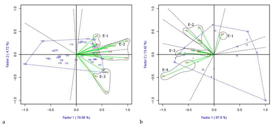
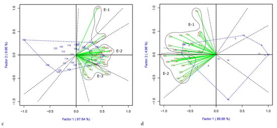
Figure 4.
GGE biplot for PGR in (a) LP and (b) in LM and for PCO (c) LP and (d) LM. The polygon (blue dotted lines) is created by connecting the varieties vector points farthest from the plot’s origin and then drawing perpendicular lines (black dotted lines) in each side of the polygon dividing it into sectors. Environments falling into one sector are grouped in the same mega-environment (E-), encircled. The blue numbers represent ryegrass varieties, whereas the red numbers and the green arrows indicate the location coordinate and the environmental vectors, respectively.
3.5. Genomic Prediction of Crown and Stem Rust Resistance
3.5.1. Variance Estimations
The estimates of variance components and phenotypic correlations for each environment are reported in Table 4. High phenotypic correlation and GEI were detected, as showed in Figure S2, where the response of few varieties is reported to demonstrate the diverse interaction responses in different environments. Indeed, all reported varieties showed a similar trend, indicating a high level of correlation, yet variability among them is detected where some were more tolerant than others.
Table 4.
Estimated variance (standard deviation) components. Location site numbers (Loc); number of tested years for a specific location (Y); phenotypic correlation among the years tested in the given location (Phen. Cor.); marker covariates (main effect) (G); average of the environments x marker interaction effect for the tested years (interaction effect “G × E”) and standard deviation (Sd); total variance (TotV) explained by the model for each location including the residual variance, which is equal to 1.
The portioning of the total genetic variance showed that the fraction of variance explained by the main effect was relatively high when the phenotypic correlation between the tested years for a given location was high. On the other hand, when the years analyzed for a particular location had low phenotypic correlation, the estimated interaction variance reported higher values (Table 4).
Overall, in the PCO dataset, the variance explained by the main effect was more significant in LM (69%) than LP (35%), reflecting the phenotypic correlation observed among the tested environments, which was on average higher in LM (0.85) than LP (0.68). Specifically, in PCO-LP, among the 16 tested locations, phenotypic correlation ranged between 0.48 of location Steinach (Germany) tested for four years and 0.85 of location Gross Luesewitz (Germany) tested for three years. The markers’ main effect explained more than 35% of the total genomic variance for locations having a weighted phenotypic correlation higher than 0.66, resulting in an interaction effect between 2% and 9% of the total genomic variance. An exception to this trend is represented by location Ottersum (Netherlands), tested for all five years, where despite the variance explained by the main effect (50%), the interaction component explained 23% of the total genetic variance due to the impact of years 2007 and 2013.
The phenotypic correlations between the 18 locations tested for PCO-LM were positively high, ranging between 0.75 in Les Rosiers (France) evaluated over four years, and 0.95 in Zurich (Switzerland) tested for all five years of the experiment. A considerable portion of the total genomic variance was explained by the main effect, ranging from 38% (Aston le Walls -UK) to 91% (Orchies -France). The interaction effect in the tested environments was slightly low and accounted for between 1% and 14%. Among the tested environments, the location Aston le Walls (UK) showed a phenotypic correlation of 0.46, and the main effect, as well as the interaction factor, explained only 10% of the total genetic variance.
In PGR-LP, the phenotypic correlation ranged from 0.41 in Lodi (Italy) to 0.85 in Zurich (Switzerland); both tested for three years. The estimations of the variance components for the eight tested locations were relatively low. For those locations with a phenotypic correlation higher than 0.64, the main effect ranged from 34% to 43% of the total genetic variance. The overall interaction effect showed a variance ranging between 3% and 13%. In the PGR-LM dataset, only one location, Hladke Zivotice (Czechia), included records for a minimum of three years. The main effect explained 63%, and the interaction effect 4% of the total genetic variance.
3.5.2. Assessment of Prediction Accuracy
The accuracy of the genomic predictions was evaluated by calculating the Brier score for each location (Table 5). Brier scores are values between 0 and 1, where values closer to 0 imply better prediction ability. Overall, the prediction accuracy was higher in locations where the phenotypic variation of the tested varieties was low within a year and across years, as reported by the coefficient of variation in Table S5.
Table 5.
Brier scores. For each location number of tested years (Y), Brier score and standard deviation (Sd) are reported. Dash refers to locations tested for less than three years for which the prediction was not computed.
For PCO, the prediction accuracies were higher in LM than LP, on average 0.39 and 0.45, respectively. In the LP population, the best prediction accuracy (0.34) was given by applying the model to Aston le Walls (UK) tested over three years. The highest Brier score, meaning the lowest prediction accuracy, was obtained for Bornhof (Germany) and Steinach (Germany) tested for four and five years, respectively. The accuracy in the PCO-LM dataset ranged between 0.42 in Aston le Walles (UK) and Pulling (Germany) tested over three and four years, respectively, and 0.48 in Les Rosiers (France) tested for four years.
In the PGR-LP data set, Brier scores ranged between 0.43 in Perugia (Italy) and 0.47 in Montours (France) tested for three and five years, whereas Hladke (Czechia) was the only one tested for three years for PGR-LM, which showed a good Brier score (0.42) compared to those given in the other data sets (Table 5).
4. Discussion
Breeding for improved rust resistance is the best way for variety improvement. One of the biggest challenges that breeders face in rust resistance breeding is the weather condition’s effect on the spreading of rust infections. Indeed, the relationship between rust disease and weather conditions has been extensively reported [55,56]. Multi environmental trials might solve this problem by testing the same varieties in different locations over multiple years and identifying ideal testing locations and mega environments where varieties perform better than others. From 2001 to 2013, as part of the EUCARPIA multi-site rust evaluation trial, a set of 54 Italian, hybrid, and perennial ryegrass varieties were tested for crown and stem rust resistance at 34 sites in 11 European countries.
4.1. AMMI and GGE Analysis of Crown and Stem Rust Disease
An essential aspect of developing new varieties in breeding programs is understanding the effect of G, E, and GEI on the variety performance. GEI represents an ideal approach for identifying and characterizing disease responses in different environmental conditions [18,20,57].
In our study, GGE analysis and AMMI were applied to evaluate the adaptability, stability, and G × E interaction effect on the crown and stem rust resistance of the 54 tested varieties. In the AMMI approach, genotype (variety) and environments explained the most significant part of the total phenotypic variance. This observation is in agreement with studies assessing GEI in fungal disease resistance responses in rice [57] and potato [19,20]. Nevertheless, variety performances were affected by the interaction with the environment; indeed, the G × E component had a consistent effect on the observed response, indicating that the best performer in one environment was not necessarily the best in another. This was confirmed by the large sum of squares of the environments, which meant that the environmental effect strongly influenced the variety’s performances. This variation could be attributed to different weather conditions in different environments when temperature, rainfall, humidity, and altitude were considered [58]. Therefore, to identify well-performing varieties in terms of high tolerance to rust diseases across multiple environments, it is crucial to consider the stability and adaptability of the tested varieties across a given geographic area. Environments where the most and least susceptible performing varieties to stem and crown rust were identified might provide useful information for local breeders in terms of sources of resistance. In two locations, Aberystwyth (UK- Wales) and Pulling (Germany), both perennial and Italian ryegrass showed higher levels of tolerance to the crown rust disease, as well as stability in the response across years. In contrast, Malchow (Germany) and Steinach (Germany) were locations where perennial and Italian ryegrass showed a high level of resistance and low variability to stem rust across years. The GEI pattern is better represented when varieties and environments are plotted considering the two first principal components of the analysis, as previously reported in sugarcane [16] and rice [59] studies. In this regard, the AMMI2 analysis might be more accurate to detect GEI variation due to information from two IPCAs. However, varieties for stable rust resistance would present a high mean resistance level and a low sensibility to environmental changes as reflected by the low slope (bi) values and IPCA scores close to zero, indicating high stability across tested environments [14].
GGE analysis assists in identifying mega-environments based on the tested variety performances and selecting the best varieties for stability and level of tolerance to the disease for a given mega-environment [22,60]. This information can be used to select discriminating and representative environments in breeding programs to identify generally adapted varieties. There was no clear indication that environments were being grouped based on their geographical location, suggesting that a more intricate combination of environmental factors, such as rainfall, temperature, and relative humidity, as well as the presence or absence of the alternative host which might increase the virulence of crown rust, may have played a key role in the phenotypic variability of the varieties and grouping of the environments.
Among the tested perennial ryegrass varieties, the one that performed best in both AMMI and GGE analysis was the Gwendal variety, showing high resistance scores to the infection and stability across environments under crown as well as stem rust. Regarding PGR, the Domino variety was the best performer among the Italian ryegrass varieties in both analyses. In contrast, Aberexcel and Tarandus were among the most tolerant varieties to PCO, being the most stable in the majority of environments under AMMI and GGE analysis, respectively. All the best performers were tetraploid; indeed, on average, tetraploid varieties showed a one unit increase in rust resistance compared to the diploids. A stronger rust tolerance is one of the features that make tetraploids better than diploids, together with a higher yield, better palatability and digestibility [61], greater grazing efficiency performances [62], and higher competitive ability [63]. Based on the results, it appears possible to breed stable varieties with high tolerance to rust disease.
This investigation represents the first study evaluating crown and stem rust resistance on different ryegrass varieties across several environments using AMMI and GGE. The results suggest that both approaches are efficient ways of assessing ryegrass varieties in a MET study to identify more stable rust resistance candidates.
4.2. Variance Components and Genomic Prediction Accuracy
Multi environmental trials result in a large amount of phenotypic data, which can be used to develop predictive models for relevant traits in ryegrasses. Several studies have shown the benefit of including marker information in G × E analysis with an extensive increase in prediction accuracy [28,29,30,31]. The M × E model described by Lopez-Cruz et al. [30] showed considerable gains in prediction accuracy compared to the single-environment analysis and a standard across-environments model. The M × E model relies on the decomposition of the genomic values into components that are stable across environments (main effect) and others that are environment-specific (interactions).
In agreement with Lopez-Cruz et al. [30], the portion of genomic variance explained by the markers’ main effect is directly related to the phenotypic correlation between years for each location. The high phenotypic correlation between years and locations confirmed the low variability of disease incidence in the tested environments, as previously described by Schubiger et al. [40]. These results can be explained by the tested sites’ geographical locations, representing central and northwest Europe. Among the tested environments, years with a lower phenotypic correlation had a more robust interaction effect than those with a high phenotypic correlation reducing the prediction accuracy. As reported previously [28,30,32,64,65], for traits with a high phenotypic correlation between environments, the M × E model captures a high total genomic variance due to the inclusion of the M × E interaction information. The presence of a significant G × E interaction in crown rust resistance was in agreement with previous studies on perennial ryegrass [37].
For each location, varieties tested in some years but not in others were predicted (CV2). The cross-validation is based on the decomposition of the marker variance in the main effects and the environment-specific marker effect, and it performed exceptionally well for all environments.
Prediction accuracy is usually evaluated by computing Pearson’s correlation between predictions and phenotypes in the testing data set [66]. However, when the phenotypic data are described using a categorical system, this assessment is not appropriate [67]; therefore, a Brier score was preferred. In this matrix system, lower values indicate a more accurate prediction. We found that in environments with a high phenotypic correlation, the interaction model explained a significantly high total variance and, therefore, genomic predictions were more accurate overall. In general, there was a good correlation between predictive ability and phenotypic variance, and this relationship has been observed previously [36,68,69].
As Lopez-Cruz et al. [30] reported, the advantage of using the M × E model in the CV2 is attributed to the possibility of borrowing information within varieties across environments. In other terms, the M × E model benefits from records of the predicted varieties collected in correlated environments.
This represents an important result for ryegrass breeding programs that aim to evaluate varieties across Europe for crown and stem rust resistance. A dense historical data set, such as the one used in our study, made it possible to have a more accurate picture of the rust disease development across years and locations, confirming the ability to use data from one environment to predict the other. Despite the limitations of this study, represented mainly by the limited number of tested varieties, this experiment has the advantage of having a high number of markers and sizeable historical data collected over multiple years and locations. To our knowledge, our study is the first one to perform genomic prediction on ryegrass using a multi-site rust evaluation trial.
5. Conclusions
This study aimed to explore the effect of the environments on the crown and stem rust resistance in different varieties of ryegrasses. The large sum of squares, as well as the significant impact of the G × E interaction, confirmed the environment’s role in the varieties’ response to the infection. The AMMI and GGE analysis gave similar results identifying the best performing varieties in terms of stability and tolerance to the pathogens across the tested environments. Our results clearly illustrate the benefit of using observations across multi environments to evaluate varieties as well as location performances.
Furthermore, our results showed that despite the limited number of genotyped individuals, the substantial number of observations across multi environments allowed us to predict crown as well as stem rust performances with moderate to high accuracy. We showed that genomic prediction using METs data could help to enhance breeding programs for the crown and stem rust in ryegrass.
Supplementary Materials
The following are available online at https://www.mdpi.com/article/10.3390/agronomy11061119/s1, Figure S1: AMMI 2 biplot, Figure S2: Response variability across environments, Table S1: List of locations tested in Europe from 2001 to 2013, Tabe S2: The adopted scoring scale reported by Schubiger et al., Table S3: Summary of perennial ryegrass varieties information, Table S4: Summary of Italian and hybrid ryegrass varieties information, Table S5: Summary of the phenotypic variation per location across years.
Author Contributions
Conceptualization, M.F., M.M. and T.A.; methodology, M.F., M.M. and T.A.; formal analysis, M.F. and M.M.; resources, T.A. and F.X.S.; writing—original draft preparation, M.F.; writing—review and editing, M.F., M.M., T.A. and F.X.S. All authors have read and agreed to the published version of the manuscript.
Funding
This research received no external funding.
Acknowledgments
We thank Stephan Hentrup for preparing the GBS libraries and members of the EUCARPIA multi-site rust evaluation consortium who took part in the phenotypic data collection.
Conflicts of Interest
The authors declare no conflict of interest.
References
- Dracatos, P.M.; Cogan, N.O.I.; Keane, P.J.; Smith, K.F.; Forster, J.W. Biology and Genetics of Crown Rust Disease in Ryegrasses. Crop Sci. 2010, 50, 1605–1624. [Google Scholar] [CrossRef]
- Potter, L.R.; Cagaś, B.; Paul, V.H.; Birckenstaedt, E. Pathogenicity of Some European Collections of Crown Rust (Puccinia coronata Corda) on Cultivars of Perennial Ryegrass. J. Phytopathol. 2008, 130, 119–126. [Google Scholar] [CrossRef]
- Kimbeng, C. Genetic basis of crown rust resistance in perennial ryegrass, breeding strategies, and genetic variation among pathogen populations: A review. Anim. Prod. Sci. 1999, 39, 361–378. [Google Scholar] [CrossRef]
- Schubiger, F.X.; Baert, J.; Bayle, B.; Bourdon, P.; Cagas, B.; Cernoch, V.; Czembor, E.; Eickmeyer, F.; Feuerstein, U.; Hartmann, S.; et al. Susceptibility of European cultivars of Italian and perennial ryegrass to crown and stem rust. Euphytica 2010, 176, 167–181. [Google Scholar] [CrossRef]
- Roderick, H.W.; Thomas, B.J. Infection of ryegrass by three rust fungi (Puccinia coronata, P. graminis and P. loliina) and some effects of temperature on the establishment of the disease and sporulation. Plant Pathol. 1997, 46, 751–761. [Google Scholar] [CrossRef]
- Pfender, W.F. Interaction of fungicide physical modes of action and plant phenology in control of stem rust of perennial ryegrass grown for seed. Plant Dis. 2006, 90, 1225–1232. [Google Scholar] [CrossRef]
- Humphreys, M.O.; Feuerstein, U.; Vandewalle, M.J.B. Ryegrasses. In Fodder Crops and Amenity Grasses. Handbook of Plant Breeding; Boller, B., Posselt, U.K., Veronesi, F., Eds.; Springer: New York, NY, USA, 2010; Volume 5, pp. 211–260. [Google Scholar]
- Peterson, P.D.; Leonard, K.J.; Roelfs, A.P.; Sutton, T.B. Effect of Barberry Eradication on Changes in Populations of Puccinia graminis in Minnesota. Plant Dis. 2005, 89, 935–940. [Google Scholar] [CrossRef]
- Park, R.F.; Wellings, C.R. Somatic Hybridization in the Uredinales. In Annual Review of Phytopathology; Van Alfen, N.K., Leach, J.E., Lindow, S., Eds.; Annual Reviews: Palo Alto, CA, USA, 2012; Volume 50, pp. 219–239. [Google Scholar]
- Kochman, J.K.; Brown, J.F. Host and environmental effects on the penetration of oats by Puccinia graminis avenae and Puccinia coronata avenae. Ann. Appl. Biol. 1976, 82, 251–258. [Google Scholar] [CrossRef]
- Naseri, B.; Sabeti, P. Analysis of the effects of climate, host resistance, maturity and sowing date on wheat stem rust epidemics. J. Plant Pathol. 2021, 103, 197–205. [Google Scholar] [CrossRef]
- Castillo, D.; Matus, I.; Del Pozo, A.; Madariaga, R.; Mellado, M. Adaptability and genotype × environment interaction of spring wheat cultivars in Chile using regression analysis, AMMI, and SREG. Chil. J. Agric. Res. 2012, 72, 167–174. [Google Scholar] [CrossRef][Green Version]
- Dia, M.; Wehner, T.C.; Perkins-Veazie, P.; Hassell, R.; Price, D.S.; Boyhan, G.E.; Olson, S.M.; King, S.R.; Davis, A.R.; Tolla, G.E.; et al. Stability of fruit quality traits in diverse watermelon cultivars tested in multiple environments. Hortic. Res. 2016, 3, 16066. [Google Scholar] [CrossRef] [PubMed]
- Guerra, E.; De Oliveira, R.; Daros, E.; Zambon, J.L.C.; Ido, O.; Bespalhok, J. Stability and adaptability of early maturing sugarcane clones by AMMI analysis. Crop Breed. Appl. Biotechnol. 2009, 9, 260–267. [Google Scholar] [CrossRef]
- Oliveira, E.J.d.; Freitas, J.P.X.d.; Jesus, O.N.d. AMMI analysis of the adaptability and yield stability of yellow passion fruit varieties. Sci. Agric. 2014, 71, 139–145. [Google Scholar] [CrossRef]
- Tena, E.; Goshu, F.; Mohamad, H.; Tesfa, M.; Tesfaye, D.; Seife, A. Genotype × environment interaction by AMMI and GGE-biplot analysis for sugar yield in three crop cycles of sugarcane (Saccharum officinirum L.) clones in Ethiopia. Cogent Food Agric. 2019, 5, 1651925. [Google Scholar] [CrossRef]
- Beyene, A.; Sibiya, J.; Derera, J.; Fikre, A. Analysis of genotype × environment interaction and stability for grain yield and chocolate spot (Botrytis fabae) disease resistance in faba bean (Vicia faba). Aust. J. Crop Sci. 2017, 11, 1228–1235. [Google Scholar]
- Das, A.; Parihar, A.K.; Saxena, D.; Singh, D.; Singha, K.D.; Kushwaha, K.P.S.; Chand, R.; Bal, R.S.; Chandra, S.; Gupta, S. Deciphering Genotype-by- Environment Interaction for Targeting Test Environments and Rust Resistant Genotypes in Field Pea (Pisum sativum L.). Front. Plant Sci. 2019, 10, 825. [Google Scholar] [CrossRef] [PubMed]
- Forbes, G.A.; Chacón, M.G.; Kirk, H.G.; Huarte, M.A.; Van Damme, M.; Distel, S.; Mackay, G.R.; Stewart, H.E.; Lowe, R.; Duncan, J.M.; et al. Stability of resistance to Phytophthora infestans in potato: An international evaluation. Plant Pathol. 2005, 54, 364–372. [Google Scholar] [CrossRef]
- Ngailo, S.; Shimelis, H.; Sibiya, J.; Mtunda, K.; Mashilo, J. Genotype-by-environment interaction of newly-developed sweet potato genotypes for storage root yield, yield-related traits and resistance to sweet potato virus disease. Heliyon 2019, 5, e01448. [Google Scholar] [CrossRef]
- Gauch, H.G. Statistical Analysis of Regional Yield Trials: AMMI Analysis of Factorial Designs; Elsevier: Amsterdam, The Netherlands, 1992; p. 278. [Google Scholar]
- Yan, W.; Kang, M.S. GGE Biplot Analysis: A Graphical Tool for Breeders, Geneticists, and Agronomist; CRC Press: Boca Raton, FL, USA, 2003. [Google Scholar]
- Gauch, H. Statistical analysis of yield trials by AMMI and GGE. Crop Sci. 2006, 46, 1488–1500. [Google Scholar] [CrossRef]
- Yan, W. GGEbiplot—A Windows Application for Graphical Analysis of Multienvironment Trial Data and Other Types of Two-Way Data. Agron. J. 2001, 93, 1111–1118. [Google Scholar] [CrossRef]
- Yan, W.; Rajcan, I. Biplot Analysis of Test Sites and Trait Relations of Soybean in Ontario. Crop Sci. 2002, 42, 11–20. [Google Scholar] [CrossRef] [PubMed]
- Yan, W.; Hunt, L.; Sheng, Q.; Szlavnics, Z. Cultivar Evaluation and Mega-Environment Investigation Based on the GGE Biplot. Crop Sci. 2000, 40, 597–605. [Google Scholar] [CrossRef]
- Meuwissen, T.H.E.; Hayes, B.J.; Goddard, M.E. Prediction of Total Genetic Value Using Genome-Wide Dense Marker Maps. Genetics 2001, 157, 1819. [Google Scholar] [CrossRef] [PubMed]
- Burgueño, J.; de los Campos, G.; Weigel, K.; Crossa, J. Genomic Prediction of Breeding Values when Modeling Genotype × Environment Interaction using Pedigree and Dense Molecular Markers. Crop Sci. 2012, 52, 707–719. [Google Scholar] [CrossRef]
- Gapare, W.; Liu, S.; Conaty, W.; Zhu, Q.-H.; Gillespie, V.; Llewellyn, D. Historical Datasets Support Genomic Selection Models for the Prediction of Cotton Fiber Quality Phenotypes Across Multiple Environments. G3 Genes Genomes Genet. 2018, 8, 1721–1732. [Google Scholar] [CrossRef]
- Lopez-Cruz, M.; Crossa, J.; Bonnett, D.; Dreisigacker, S.; Poland, J.; Jannink, J.-L. Increased Prediction Accuracy in Wheat Breeding Trials Using a Marker × Environment Interaction Genomic Selection Model. G3 Genes Genomes Genet. 2015, 5, 569. [Google Scholar] [CrossRef] [PubMed]
- Sukumaran, S.; Crossa, J.; Jarquin, D.; Lopes, M.; Reynolds, M.P. Genomic Prediction with Pedigree and Genotype × Environment Interaction in Spring Wheat Grown in South and West Asia, North Africa, and Mexico. G3 Genes Genomes Genet. 2017, 7, 481–495. [Google Scholar] [CrossRef]
- Jarquín, D.; Crossa, J.; Lacaze, X.; Du Cheyron, P.; Daucourt, J.; Lorgeou, J.; Piraux, F.; Guerreiro, L.; Pérez, P.; Calus, M.; et al. A reaction norm model for genomic selection using high-dimensional genomic and environmental data. Theor. Appl. Genet. 2014, 127, 595–607. [Google Scholar] [CrossRef]
- Moreau, L.; Charcosset, A.; Gallais, A. Use of trial clustering to study QTL x environment effects for grain yield and related traits in maize. Theor. Appl. Genet. 2004, 100, 92–105. [Google Scholar] [CrossRef]
- Crossa, J.; de los Campos, G.; Maccaferri, M.; Tuberosa, R.; Burgueño, J.; Pérez-Rodríguez, P. Extending the Marker × Environment Interaction Model for Genomic-Enabled Prediction and Genome-Wide Association Analysis in Durum Wheat. Crop Sci. 2016, 56, 2193–2209. [Google Scholar] [CrossRef]
- Cuevas, J.; Crossa, J.; Soberanis, V.; Pérez-Elizalde, S.; Pérez-Rodríguez, P.; Campos, G.d.l. Genomic Prediction of Genotype × Environment Interaction Kernel Regression Models. Plant Genome 2016, 9. [Google Scholar] [CrossRef]
- Arojju, S.K.; Conaghan, P.; Barth, S.; Milbourne, D.; Casler, M.D.; Hodkinson, T.R. Genomic prediction of crown rust resistance in Lolium perenne. BMC Genet. 2018, 19, 35. [Google Scholar] [CrossRef]
- Fè, D.; Ashraf, B.H.; Pedersen, M.G.; Janss, L.; Byrne, S.; Roulund, N.; Lenk, I.; Didion, T.; Asp, T.; Jensen, C.S.; et al. Accuracy of Genomic Prediction in a Commercial Perennial Ryegrass Breeding Program. Plant Genome 2016. [Google Scholar] [CrossRef]
- Fè, D.; Cericola, F.; Byrne, S.; Lenk, I.; Ashraf, B.H.; Pedersen, M.G.; Roulund, N.; Asp, T.; Janss, L.; Jensen, C.S.; et al. Genomic dissection and prediction of heading date in perennial ryegrass. BMC Genom. 2015, 16, 921. [Google Scholar] [CrossRef] [PubMed]
- Guo, X.Y.; Cericola, F.; Fe, D.; Pedersen, M.G.; Lenk, I.; Jensen, C.S.; Jensen, J.; Janss, L.L. Genomic Prediction in Tetraploid Ryegrass Using Allele Frequencies Based on Genotyping by Sequencing. Front. Plant Sci. 2018, 9, 14. [Google Scholar] [CrossRef] [PubMed]
- Schubiger, F.X.; Baert, J.; Ball, T.; Both, Z.; Czembor, E.; Feuerstein, U.; Hartmann, S.; Krautzer, B.; Leenheer, H.; Persson, C.; et al. (Eds.) The EUCARPIA Multi-site Rust Evaluation—2013 Results. Breeding in a World of Scarcity; Springer International Publishing: Cham, Switzerland, 2016. [Google Scholar]
- Stoffel, M.A.; Nakagawa, S.; Schielzeth, H. rptR: Repeatability estimation and variance decomposition by generalized linear mixed-effects models. Methods Ecol. Evol. 2017, 8, 1639–1644. [Google Scholar] [CrossRef]
- Gollob, H.F. A statistical model which combines features of factor analytic and analysis of variance techniques. Psychometrika 1968, 33, 73–115. [Google Scholar] [CrossRef] [PubMed]
- Pacheco, A.; Vargas, M.; Alvarado, G.; Rodríguez, F.; López, M.; Crossa, J. EA-R (Genotype x Environment Analysis whit R for Windows). Version 4.1; International Maize and Wheat Improvement Center: Mexico City, Mexico, 2016. [Google Scholar]
- Purchase, J.L.; Hatting, H.; van Deventer, C.S. Genotype × environment interaction of winter wheat (Triticum aestivum L.) in South Africa: II. Stability analysis of yield performance. South Afr. J. Plant Soil 2000, 17, 101–107. [Google Scholar] [CrossRef]
- Mendiburu, F.d. Agricolae: Statistical Procedures for Agricultural Research. R Package Version 1.3-1 2019. Available online: https://CRAN.R-project.org/package=agricolae (accessed on 20 July 2020).
- Byrne, S.; Czaban, A.; Studer, B.; Panitz, F.; Bendixen, C.; Asp, T. Genome Wide Allele Frequency Fingerprints (GWAFFs) of Populations via Genotyping by Sequencing. PLoS ONE 2013, 8, e57438. [Google Scholar] [CrossRef]
- Elshire, R.J.; Glaubitz, J.C.; Sun, Q.; Poland, J.A.; Kawamoto, K.; Buckler, E.S.; Mitchell, S.E. A Robust, Simple Genotyping-by-Sequencing (GBS) Approach for High Diversity Species. PLoS ONE 2011, 6, e19379. [Google Scholar] [CrossRef]
- Joshi, N.A.; Fass, J.N. Sickle: A Sliding-Window, Adaptive, Quality-Based Trimming Tool for FastQ files (Version 1.33). 2011. Available online: https://github.com/najoshi/sickle (accessed on 30 May 2021).
- Li, H.; Durbin, R. Fast and accurate short read alignment with Burrows-Wheeler transform. Bioinformatics 2009, 25, 1754–1760. [Google Scholar] [CrossRef] [PubMed]
- Poplin, R.; Ruano-Rubio, V.; DePristo, M.A.; Fennell, T.J.; Carneiro, M.O.; Van der Auwera, G.A.; Kling, D.E.; Gauthier, L.D.; Levy-Moonshine, A.; Roazen, D.; et al. Scaling accurate genetic variant discovery to tens of thousands of samples. bioRxiv 2018. [Google Scholar] [CrossRef]
- Danecek, P.; Auton, A.; Abecasis, G.; Albers, C.A.; Banks, E.; DePristo, M.A.; Handsaker, R.E.; Lunter, G.; Marth, G.T.; Sherry, S.T.; et al. The variant call format and VCFtools. Bioinformatics 2011, 27, 2156–2158. [Google Scholar] [CrossRef] [PubMed]
- Pérez, P.; de los Campos, G. Genome-wide regression and prediction with the BGLR statistical package. Genetics 2014, 198, 483–495. [Google Scholar] [CrossRef] [PubMed]
- Roorkiwal, M.; Jarquin, D.; Singh, M.K.; Gaur, P.M.; Bharadwaj, C.; Rathore, A.; Howard, R.; Srinivasan, S.; Jain, A.; Garg, V.; et al. Genomic-enabled prediction models using multi-environment trials to estimate the effect of genotype × environment interaction on prediction accuracy in chickpea. Sci. Rep. 2018, 8, 1–11. [Google Scholar] [CrossRef] [PubMed]
- Brier, G.W. Verification of forecast expressed in terms of probability. Mon. Weather Rev. 1950, 78, 1–3. [Google Scholar] [CrossRef]
- Caubel, J.; Launay, M.; Ripoche, D.; Gouache, D.; Buis, S.; Huard, F. Climate change effects on leaf rust of wheat: Implementing a coupled crop-disease model in a French regional application. Eur. J. Agron. 2017, 90, 53–66. [Google Scholar] [CrossRef]
- Junk, J.; Kouadio, L.; Delfosse, P.; El Jarroudi, M. Effects of regional climate change on brown rust disease in winter wheat. Clim. Chang. 2016, 135, 439–451. [Google Scholar] [CrossRef]
- Mukherjee, A.; Nk, M.; Bose, L.; Jambhulkar, N.; Nayak, P. Additive main effects and multiplicative interaction (AMMI) analysis of GxE interactions in rice-blast pathosystem to identify stable resistant genotypes. Afr. J. Agric. Res. 2013, 8, 5492–5507. [Google Scholar]
- Balfourier, F.; Charmet, G. Relationships between agronomic characters and ecogeographical factors in a collection of French perennial ryegrass populations. Agronomie 1991, 11, 645–657. [Google Scholar] [CrossRef]
- Samonte, S.O.; Wilson, L.; McClung, A.; Medley, J. Targeting cultivars onto rice growing environments using AMMI and SREG GGE biplot analyses. Crop Sci. 2005, 45, 2414–2424. [Google Scholar] [CrossRef]
- Mattos, P.; De Oliveira, R.; Bespalhok, J.; Daros, E.; Verissimo, M. Evaluation of sugarcane genotypes and production environments in Paraná by GGE biplot and AMMI analysis. Crop Breed. Appl. Biotechnol. 2013, 13, 83–90. [Google Scholar] [CrossRef]
- Wilkins, P.W. Breeding perennial ryegrass for agriculture. Euphytica 1991, 52, 201–214. [Google Scholar] [CrossRef]
- Tubritt, T.; Delaby, L.; Gilliland, T.; O’Donovan, M. An investigation into the grazing efficiency of perennial ryegrass varieties. Grass Forage Sci. 2020, 75, 253–265. [Google Scholar] [CrossRef]
- Sugiyama, S. Differentiation in competitive ability and cold tolerance between diploid and tetraploid cultivars in Lolium perenne. Euphytica 1998, 103, 55–59. [Google Scholar] [CrossRef]
- Cuevas, J.; Crossa, J.A.-O.; Montesinos-López, O.A.; Burgueño, J.; Pérez-Rodríguez, P.; de Los Campos, G. Bayesian Genomic Prediction with Genotype × Environment Interaction Kernel Models. G3 Genes Genomes Genet. 2017, 7, 41–53. [Google Scholar] [CrossRef] [PubMed]
- Richards, C.L.; Alonso, C.; Becker, C.; Bossdorf, O.; Bucher, E.; Colome-Tatche, M.; Durka, W.; Engelhardt, J.; Gaspar, B.; Gogol-Doring, A.; et al. Ecological plant epigenetics: Evidence from model and non-model species, and the way forward. Ecol. Lett. 2017, 20, 1576–1590. [Google Scholar] [CrossRef]
- González-Recio, O.; Rosa, G.J.M.; Gianola, D. Machine learning methods and predictive ability metrics for genome-wide prediction of complex traits. Livest. Sci. 2014, 166, 217–231. [Google Scholar] [CrossRef]
- Montesinos-López, O.A.; Montesinos-López, A.; Pérez-Rodríguez, P.; de Los Campos, G.; Eskridge, K.; Crossa, J. Threshold models for genome-enabled prediction of ordinal categorical traits in plant breeding. G3 Genes Genomes Genet. 2015, 5, 291–300. Available online: http://europepmc.org/abstract/MED/25538102 (accessed on 31 January 2020). [CrossRef]
- Isidro, J.; Jannink, J.-L.; Akdemir, D.; Poland, J.; Heslot, N.; Sorrells, M.E. Training set optimization under population structure in genomic selection. Theor. Appl. Genet. 2015, 128, 145–158. [Google Scholar] [CrossRef] [PubMed]
- Muranty, H.; Troggio, M.; Sadok, I.B.; Rifaï, M.A.; Auwerkerken, A.; Banchi, E.; Velasco, R.; Stevanato, P.; van de Weg, W.E.; Di Guardo, M.; et al. Accuracy and responses of genomic selection on key traits in apple breeding. Hortic. Res. 2015, 2, 15060. Available online: http://europepmc.org/abstract/MED/26744627 (accessed on 7 March 2021). [CrossRef] [PubMed]
Publisher’s Note: MDPI stays neutral with regard to jurisdictional claims in published maps and institutional affiliations. |
© 2021 by the authors. Licensee MDPI, Basel, Switzerland. This article is an open access article distributed under the terms and conditions of the Creative Commons Attribution (CC BY) license (https://creativecommons.org/licenses/by/4.0/).