
Detecting the Early Flowering Stage of Tea Chrysanthemum Using the F-YOLO Model


Abstract
:1. Introduction
- A fusion detection model was designed that alternates between cross-stage partial DenseNet (CSPDenseNet) and cross-stage partial ResNeXt (CSPResNeXt) as the main network, and is equipped with several combination modules. The model can achieve abundant gradient combinations and effectively truncate the redundant gradient flow;
- We studied the impact of different data enhancement methods, feature fusion components, dataset sizes, and complex unstructured scenarios on the performance of the F-YOLO model, and proved the superiority of the F-YOLO model by comparing it with a number of state-of-the-art detection models;
- A lightweight detection model was designed for detecting chrysanthemum at the early flowering stage, which can adapt to complex unstructured environments (illumination variation, occlusion, overlapping, etc.). Anyone can train an accurate and super-fast object detector using a common mobile GPU, such as the 1080 Ti.
2. Materials and Methods
2.1. Experimental Setup
2.2. Dataset
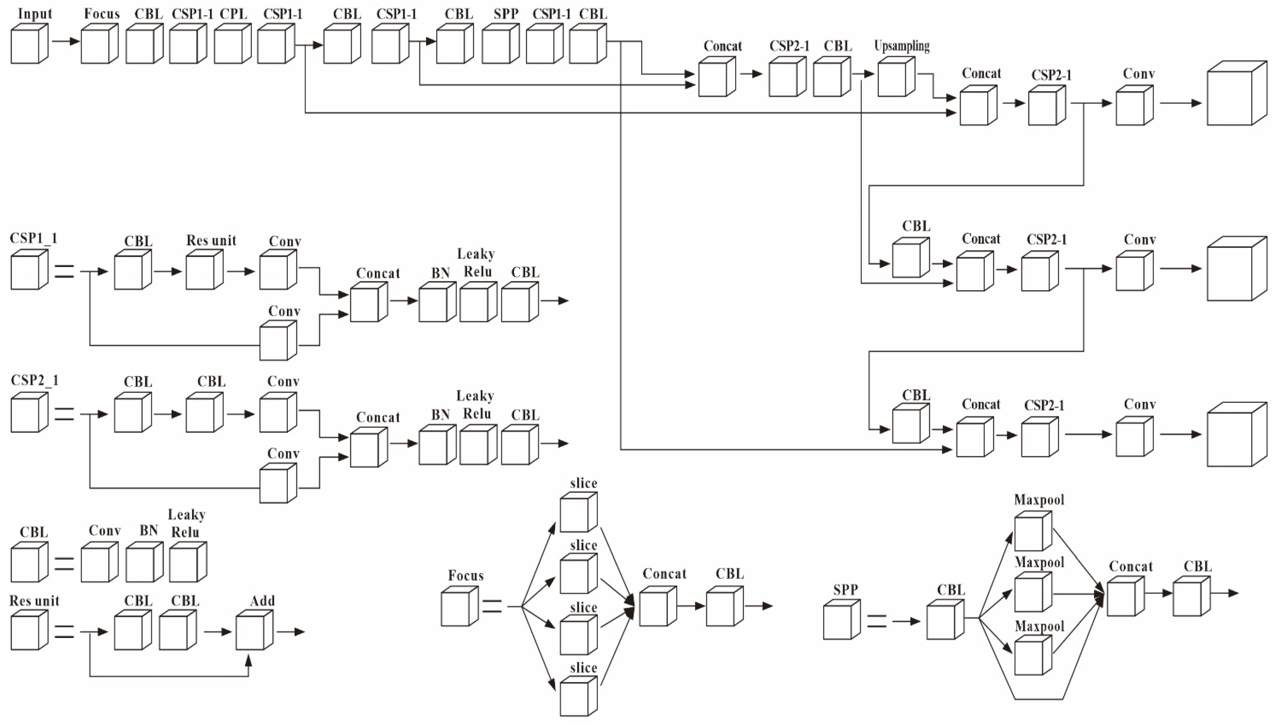
2.3. Backbone
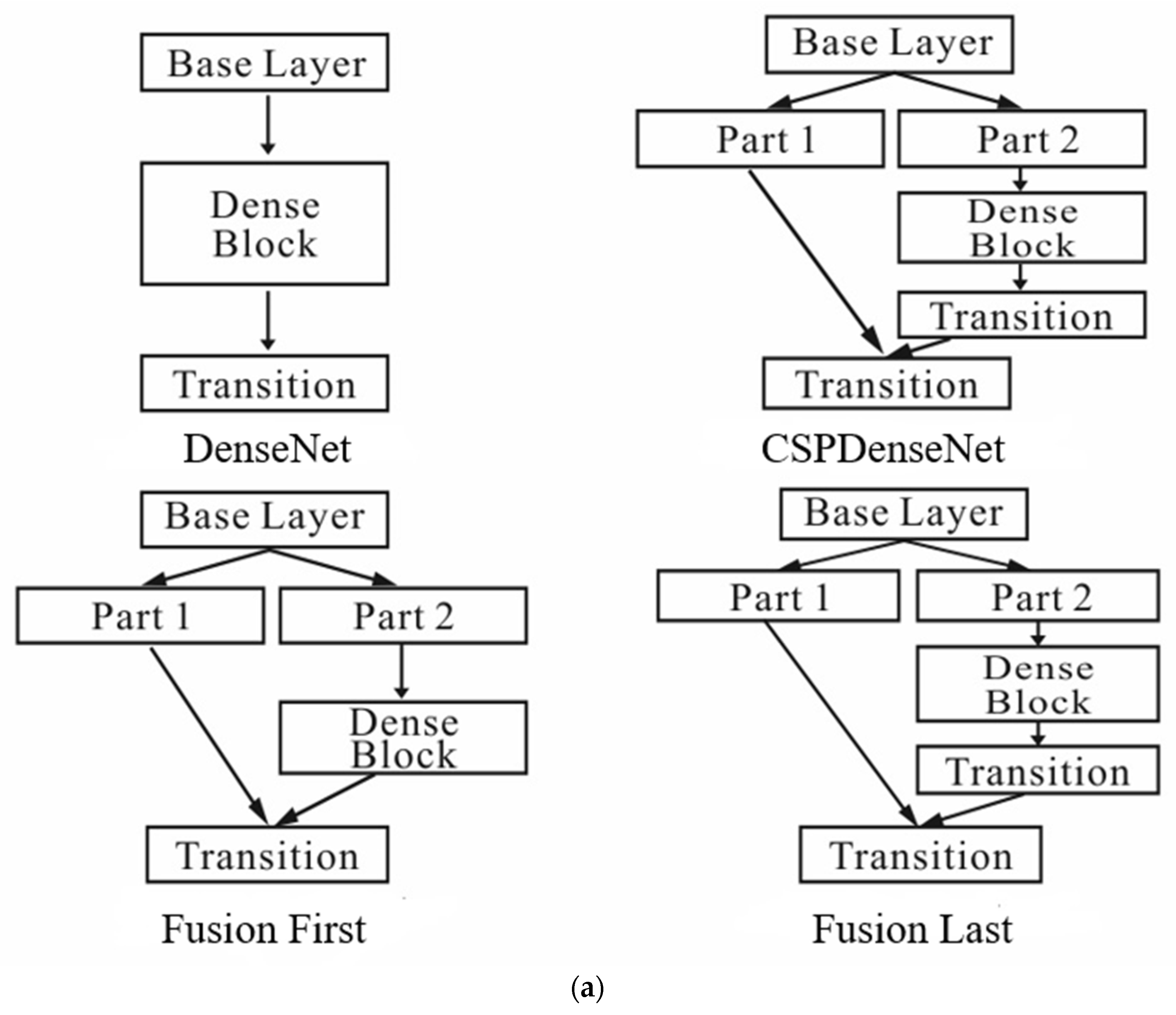
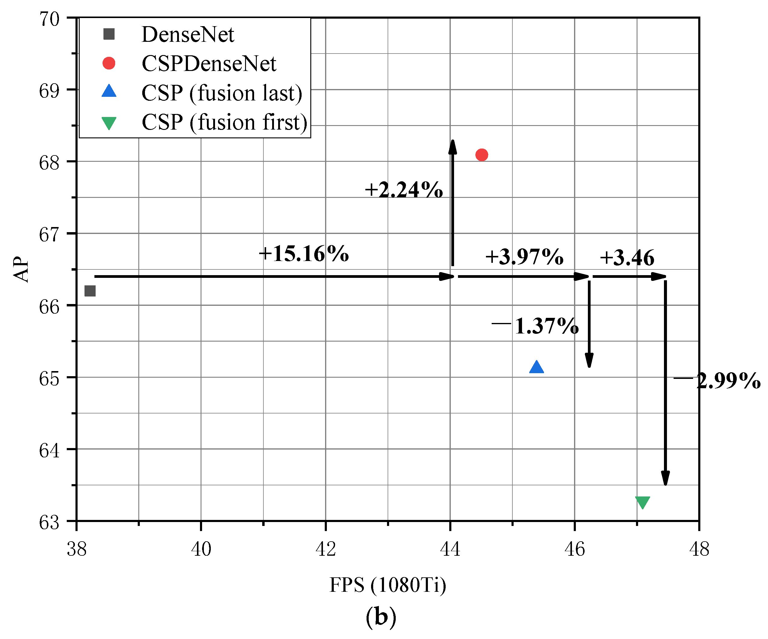
2.3.1. CSPDenseNet
2.3.2. Partial Dense Block
2.3.3. Partial Transition Layer
2.3.4. CBL + SPP
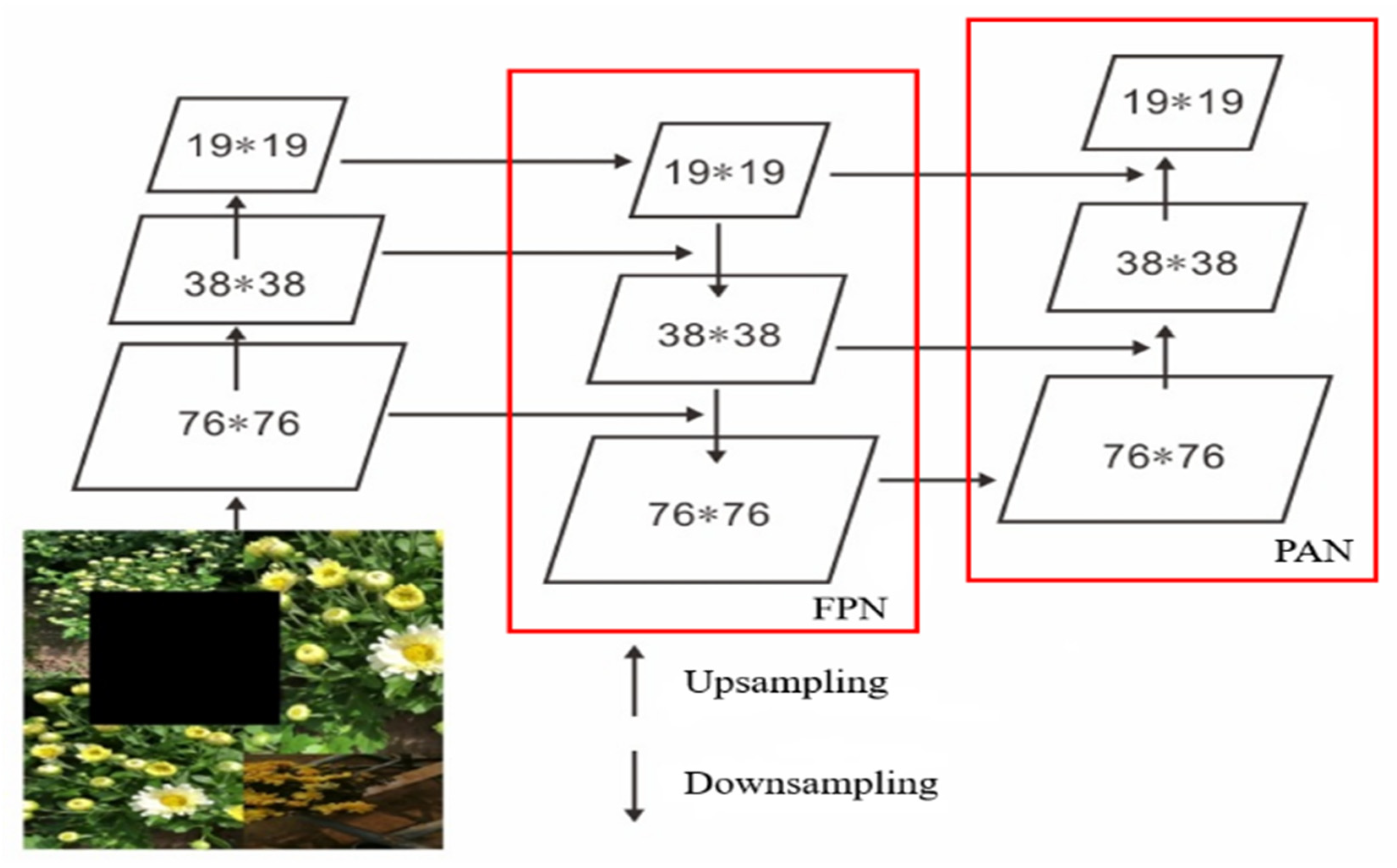
2.4. Neck
2.5. Head
3. Results
3.1. Ablation Experiments
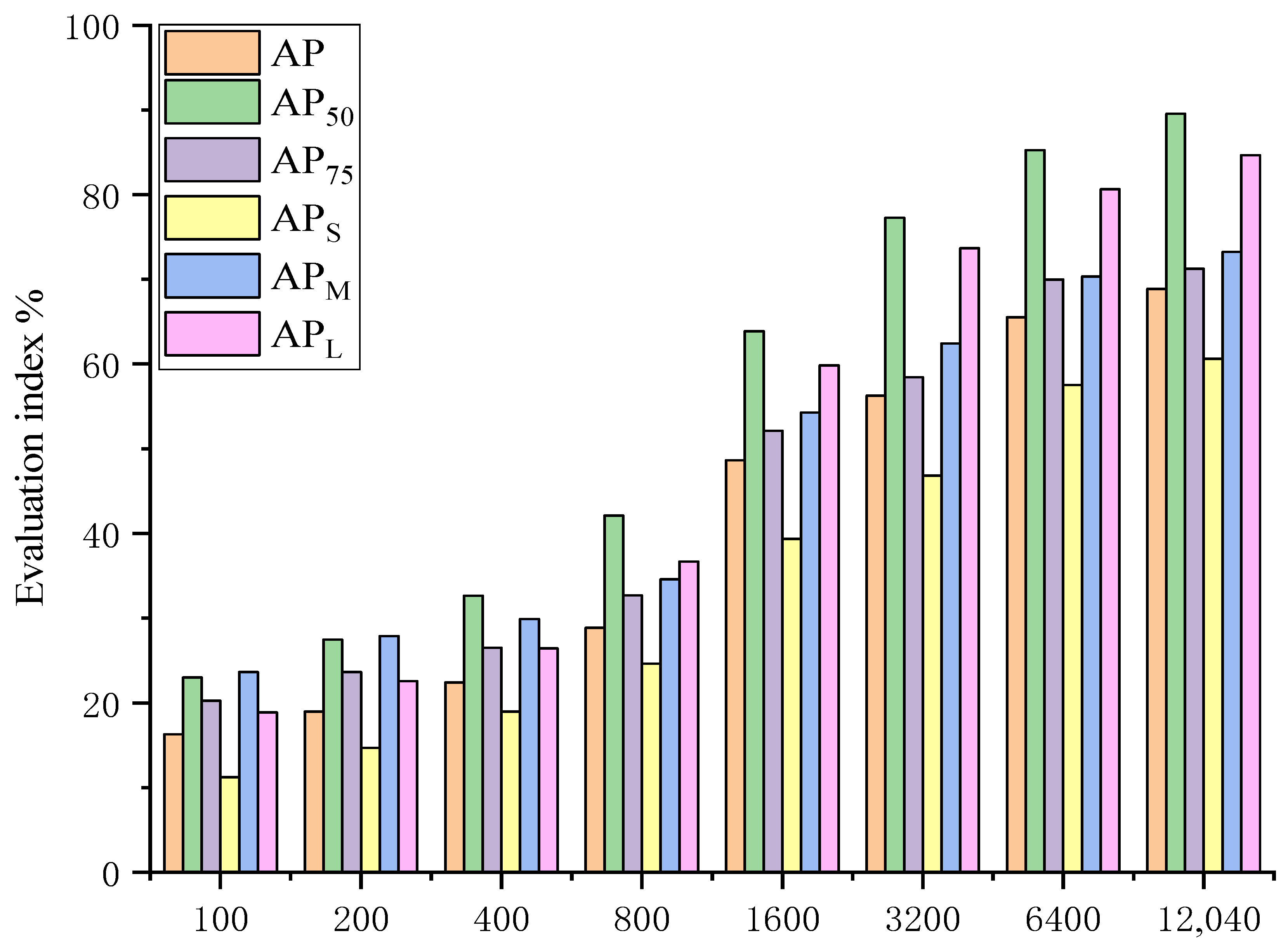
3.2. Impact of Dataset Size on the Detection Task
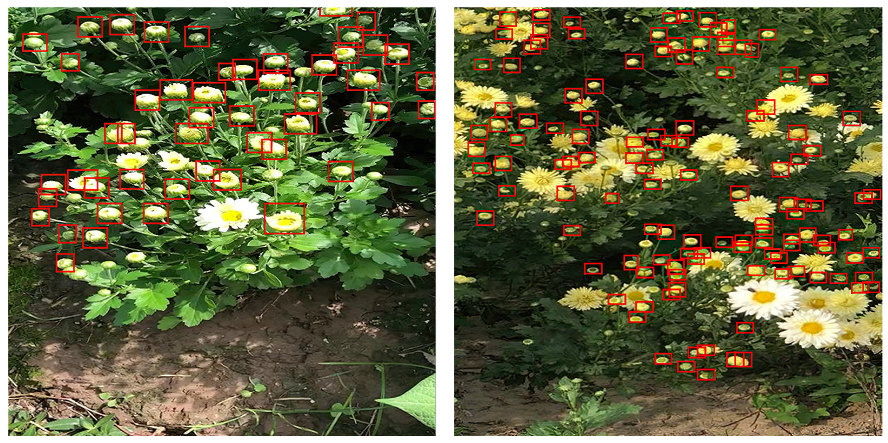
3.3. Impact of Different Unstructured Scenarios on the Detection Task
3.4. Comparisons with State-of-the-Art Detection Methods
4. Conclusions
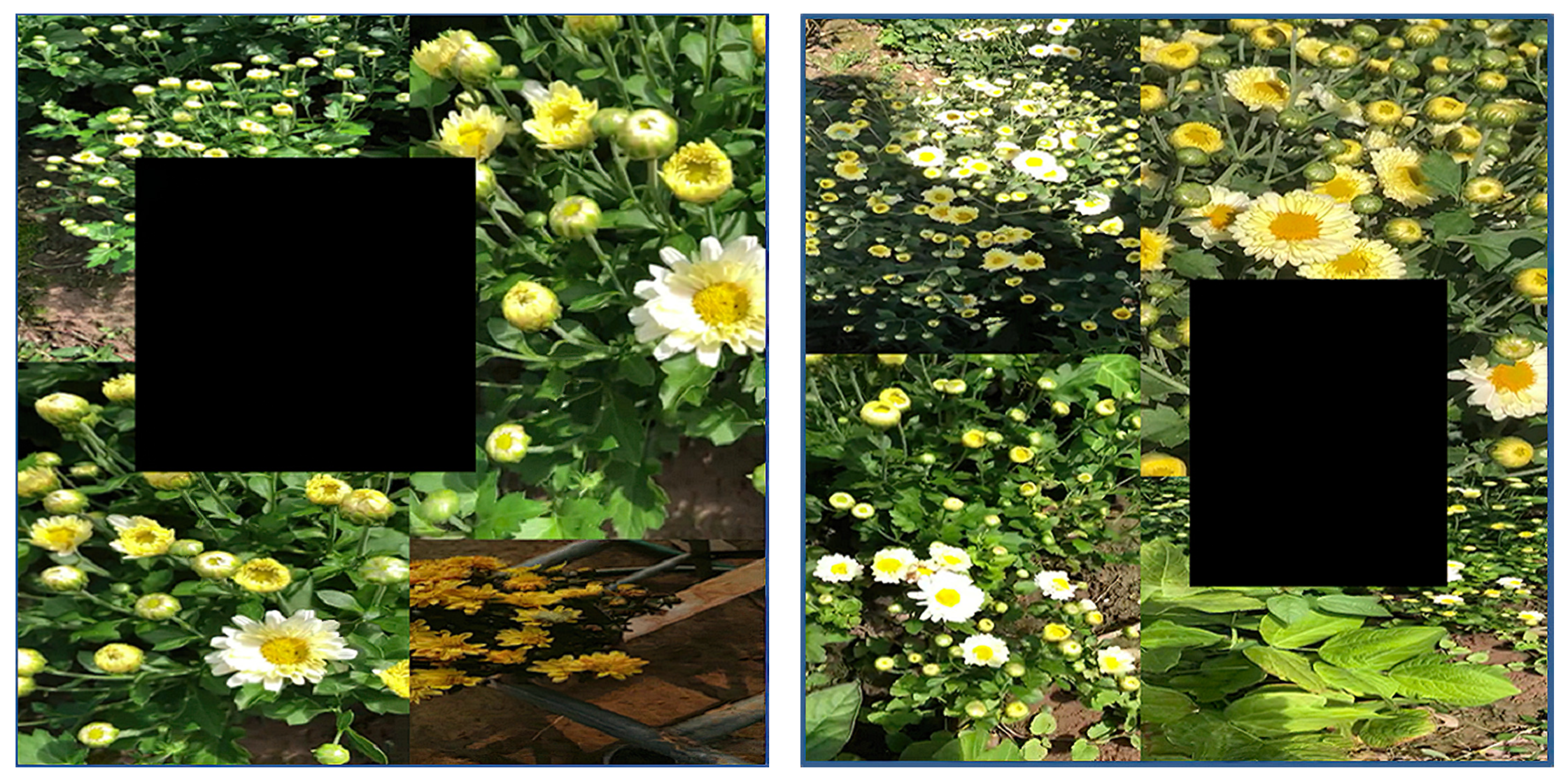
- We verified the impact of data enhancement; feature fusion; dataset size; and complex, unstructured scenarios (illumination variation, overlap, and occlusion) on the proposed F-YOLO model. The data enhancement input component equipped with cutout and mosaic achieved the best AP performance of 68.87%. The feature fusion component equipped with CSPResNeXt, SPP, and PAN achieved the best AP performance of 68.87%. The dataset size has a significant effect on the performance of the F-YOLO model, especially for large-sized objects, where the AP increased by 348.73%. In complex, unstructured environments, illumination has the least influence on the detection of chrysanthemums at the early flowering stage. Under strong light, the accuracy, error rate, and miss rate were 88.52%, 5.26%, and 6.22%, respectively. Overlapping has the biggest effect on the detection of chrysanthemums at the early flowering stage. With overlapping, the accuracy, error rate, and miss rate were 86.36%, 2.96%, and 10.68%, respectively;
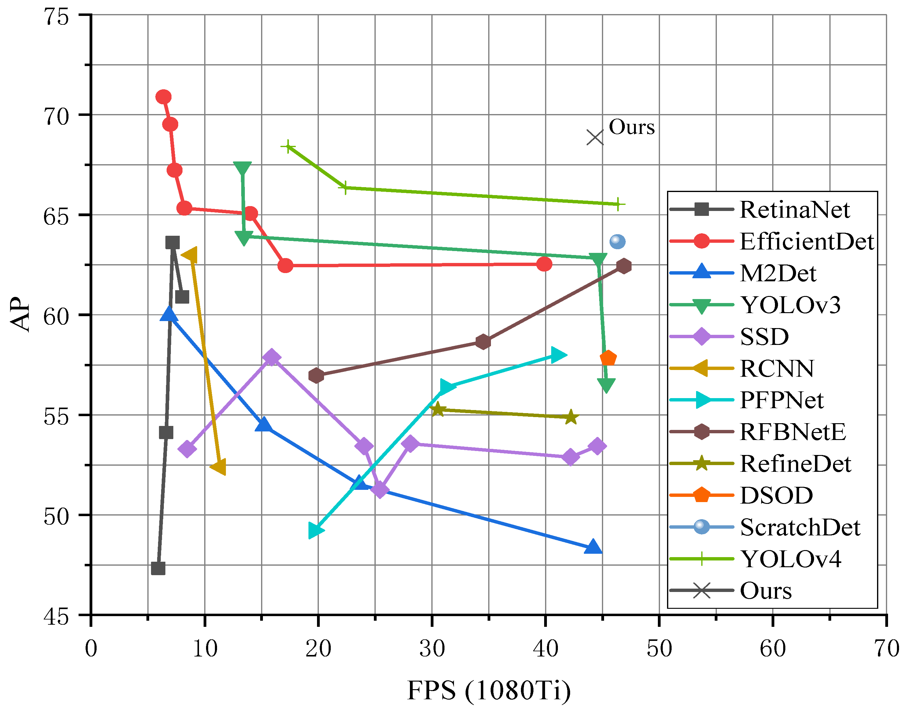
- We compared the performances of the 41 latest object detection technologies, including 12 series model frameworks and the F-YOLO model proposed in this paper. The detection rate FPS of the proposed model was not significantly improved compared with the other latest object detection technologies, but six performance indexes—namely AP, AP50, AP75, APS, APM, and APL—were significantly improved, and were 0.46%, 1.19%, 1.02%, 0.36%, 5.6%, and 4.41% higher, respectively, than those of the top-performing regional detection model YOLOv4, based on feature fusion in the experiments. In particular, for medium-sized objects, the detection performance APM reached 73.22%;
- The proposed lightweight model F-YOLO can realize automatic harvesting of chrysanthemums for tea at the early flowering stage, in order to replace manual harvesting. This method can solve the current global situation of relying on manual harvesting of chrysanthemums for tea. Based on the speed and accuracy results from our method, we believe that the advancement of new deep learning architecture and mobile computing devices, together with a large amount of field data, will significantly contribute the development of precision agriculture like chrysanthemum-picking robots in the coming years.
Author Contributions
Funding
Institutional Review Board Statement
Informed Consent Statement
Data Availability Statement
Acknowledgments
Conflicts of Interest
Abbreviations
| Full Name | Acronym |
| Fusion-YOLO | F-YOLO |
| Convolutional neural network | CNN |
| Spatial pyramid pooling | SPP |
| Pyramid pooling module | PPM |
| Atrous spatial pyramid pooling | ASPP |
| Detection with Enriched Semantics | DES |
| Feature pyramid networks | FPN |
| Single Shot multi-box detector | SSD |
| Neural architecture search | NAS |
| Cross-stage partial Densenet | CSPDenseNet |
| Cross-stage partial Resnext | CSPResNeXt |
| Non-maximum suppression | NMS |
| Distance intersection over union | DIOU |
| Stochastic gradient descent | SGD |
| Application-specified integrated circuits | ASICs |
| Perceptual adversarial network | PAN |
| Average precision | AP |
| Parallel feature pyramid network | PFPNet |
| Intersection over union | IOU |
| Multi-level feature pyramid network | MLFPN |
| Modified sine cosine algorithm | MSCA |
| Object detection module | ODM |
References
- Zhang, B.; Xie, Y.; Zhou, J.; Wang, K.; Zhang, Z. State-of-the-art robotic grippers, grasping and control strategies, as well as their applications in agricultural robots: A review. Comput. Electron. Agric. 2020, 177, 105694. [Google Scholar] [CrossRef]
- Ravankar, A.; Ravankar, A.A.; Watanabe, M.; Hoshino, Y.; Rawankar, A. Development of a Low-Cost Semantic Monitoring System for Vineyards Using Autonomous Robots. Agriculture 2020, 10, 182. [Google Scholar] [CrossRef]
- Reiser, D.; Sehsah, E.; Bumann, O.; Morhard, J.; Griepentrog, H.W. Development of an Autonomous Electric Robot Implement for Intra-Row Weeding in Vineyards. Agriculture 2019, 9, 18. [Google Scholar] [CrossRef] [Green Version]
- Ngugi, L.C.; Abdelwahab, M.; Abo-Zahhad, M. Tomato leaf segmentation algorithms for mobile phone applications using deep learning. Comput. Electron. Agric. 2020, 178, 105788. [Google Scholar] [CrossRef]
- Adhitya, Y.; Prakosa, S.W.; Koppen, M.; Leu, J.S. Feature Extraction for Cocoa Bean Digital Image Classification Prediction for Smart Farming Application. Agronomy 2020, 10, 1642. [Google Scholar] [CrossRef]
- Yang, K.L.; Zhong, W.Z.; Li, F.G. Leaf Segmentation and Classification with a Complicated Background Using Deep Learning. Agronomy 2020, 10, 1721. [Google Scholar] [CrossRef]
- Zhao, B.Q.; Li, J.T.; Baenziger, P.S.; Belamkar, V.; Ge, Y.F.; Zhang, J.; Shi, Y.Y. Automatic Wheat Lodging Detection and Mapping in Aerial Imagery to Support High-Throughput Phenotyping and In-Season Crop Management. Agronomy 2020, 10, 1762. [Google Scholar] [CrossRef]
- Villacres, J.F.; Cheein, F.A. Detection and Characterization of Cherries: A Deep Learning Usability Case Study in Chile. Agronomy 2020, 10, 835. [Google Scholar] [CrossRef]
- Wu, Y.; Xu, L.H. Crop Organ Segmentation and Disease Identification Based on Weakly Supervised Deep Neural Network. Agronomy 2019, 9, 21. [Google Scholar] [CrossRef] [Green Version]
- Song, C.M.; Kim, J.S. Applicability Evaluation of the Hydrological Image and Convolution Neural Network for Prediction of the Biochemical Oxygen Demand and Total Phosphorus Loads in Agricultural Areas. Agriculture 2020, 10, 529. [Google Scholar] [CrossRef]
- Guo, P.F.; Zeng, D.L.; Tian, Y.B.; Liu, S.Y.; Liu, H.T.; Li, D.L. Multi-scale enhancement fusion for underwater sea cucumber images based on human visual system modelling. Comput. Electron. Agric. 2020, 175, 105608. [Google Scholar] [CrossRef]
- Yin, H.; Gu, Y.H.; Park, C.J.; Park, J.H.; Yoo, S.J. Transfer Learning-Based Search Model for Hot Pepper Diseases and Pests. Agriculture 2020, 10, 439. [Google Scholar] [CrossRef]
- Hong, S.J.; Kim, S.Y.; Kim, E.; Lee, C.H.; Lee, J.S.; Lee, D.S.; Bang, J.; Kim, G. Moth Detection from Pheromone Trap Images Using Deep Learning Object Detectors. Agriculture 2020, 10, 12. [Google Scholar] [CrossRef]
- Liu, M.; Guan, H.; Ma, X.; Yu, S.; Liu, G. Recognition method of thermal infrared images of plant canopies based on the characteristic registration of heterogeneous images. Comput. Electron. Agric. 2020, 177, 105678. [Google Scholar] [CrossRef]
- Li, Y.; Chao, X.W. ANN-Based Continual Classification in Agriculture. Agriculture 2020, 10, 178. [Google Scholar] [CrossRef]
- Dai, J.; Guo, L.; Wang, Z.; Liu, S. An Orientation-correction Detection Method for Scene Text Based on SPP-CNN. In Proceedings of the 2019 IEEE 4th International Conference on Cloud Computing and Big Data Analysis (ICCCBDA), Chengdu, China, 12–15 April 2019; pp. 671–675. [Google Scholar]
- Ke, Z.; Le, C.; Yao, Y. A multivariate grey incidence model for different scale data based on spatial pyramid pooling. J. Syst. Eng. Electron. 2020, 31, 770–779. [Google Scholar] [CrossRef]
- Tian, Y.; Chen, F.; Wang, H.; Zhang, S. Real-Time Semantic Segmentation Network Based on Lite Reduced Atrous Spatial Pyramid Pooling Module Group. In Proceedings of the 2020 5th International Conference on Control, Robotics and Cybernetics (CRC), Wuhan, China, 16–18 October 2020; pp. 139–143. [Google Scholar]
- Won, J.; Lee, D.; Lee, K.; Lin, C. An Improved YOLOv3-based Neural Network for De-identification Technology. In Proceedings of the 2019 34th International Technical Conference on Circuits/Systems, Computers and Communications (ITC-CSCC), JeJu, Korea, 23–26 June 2019; pp. 1–2. [Google Scholar]
- Zhang, Z.; Qiao, S.; Xie, C.; Shen, W.; Wang, B.; Yuille, A.L. Single-Shot Object Detection with Enriched Semantics. In Proceedings of the 2018 IEEE/CVF Conference on Computer Vision and Pattern Recognition, Salt Lake City, UT, USA, 18–23 June 2018; pp. 5813–5821. [Google Scholar]
- Kang, M.; Kim, H.; Kang, D. Finding a High Accuracy Neural Network for the Welding Defects Classification Using Efficient Neural Architecture Search via Parameter Sharing. In Proceedings of the 2018 18th International Conference on Control, Automation and Systems (ICCAS), PyeongChang, Korea, 17–20 October 2018; pp. 402–405. [Google Scholar]
- Wang, C.; Liao, H.M.; Wu, Y.; Chen, P.; Hsieh, J.; Yeh, I. CSPNet: A New Backbone that can Enhance Learning Capability of CNN. In Proceedings of the 2020 IEEE/CVF Conference on Computer Vision and Pattern Recognition Workshops (CVPRW), Seattle, WA, USA, 14–19 June 2020; pp. 1571–1580. [Google Scholar]
- Chen, C.; Zhu, W.; Steibel, J.; Siegford, J.; Han, J.; Norton, T. Recognition of feeding behaviour of pigs and determination of feeding time of each pig by a video-based deep learning method. Comput. Electron. Agric. 2020, 176, 105642. [Google Scholar] [CrossRef]
- Kuznetsova, A.; Maleva, T.; Soloviev, V. Using YOLOv3 Algorithm with Pre- and Post-Processing for Apple Detection in Fruit-Harvesting Robot. Agronomy 2020, 10, 1016. [Google Scholar] [CrossRef]
- Zhang, C.L.; Zou, K.L.; Pan, Y. A Method of Apple Image Segmentation Based on Color-Texture Fusion Feature and Machine Learning. Agronomy 2020, 10, 972. [Google Scholar] [CrossRef]
- Koirala, A.; Walsh, K.B.; Wang, Z.L.; Anderson, N. Deep Learning for Mango (Mangifera indica) Panicle Stage Classification. Agronomy 2020, 10, 143. [Google Scholar] [CrossRef] [Green Version]
- Mao, S.H.; Li, Y.H.; Ma, Y.; Zhang, B.H.; Zhou, J.; Wang, K. Automatic cucumber recognition algorithm for harvesting robots in the natural environment using deep learning and multi-feature fusion. Comput. Electron. Agric. 2020, 170, 105254. [Google Scholar] [CrossRef]
- Yaramasu, R.; Bandaru, V.; Pnvr, K. Pre-season crop type mapping using deep neural networks. Comput. Electron. Agric. 2020, 176, 105664. [Google Scholar] [CrossRef]
- Jang, W.S.; Lee, Y.; Neff, J.C.; Im, Y.; Ha, S.; Doro, L. Development of an EPIC parallel computing framework to facilitate regional/global gridded crop modeling with multiple scenarios: A case study of the United States. Comput. Electron. Agric. 2019, 158, 189–200. [Google Scholar] [CrossRef]
- Cruz Ulloa, C.; Krus, A.; Barrientos, A.; Del Cerro, J.; Valero, C. Robotic Fertilisation Using Localisation Systems Based on Point Clouds in Strip-Cropping Fields. Agronomy 2021, 11, 11. [Google Scholar] [CrossRef]
- Kim, W.S.; Lee, D.H.; Kim, Y.J.; Kim, Y.S.; Kim, T.; Park, S.U.; Kim, S.S.; Hong, D.-H. Crop Height Measurement System Based on 3D Image and Tilt Sensor Fusion. Agronomy 2020, 10, 1670. [Google Scholar] [CrossRef]
- Wang, Y.; Wang, L.; Jiang, Y.; Li, T. Detection of Self-Build Data Set Based on YOLOv4 Network. In Proceedings of the 2020 IEEE 3rd International Conference on Information Systems and Computer Aided Education (ICISCAE), Dalian, China, 27–29 September 2020; pp. 640–642. [Google Scholar]
- Kumar, C.; Punitha, R. YOLOv3 and YOLOv4: Multiple Object Detection for Surveillance Applications. In Proceedings of the 2020 Third International Conference on Smart Systems and Inventive Technology (ICSSIT), Tirunelveli, India, 20–22 August 2020; pp. 1316–1321. [Google Scholar]
- Sung, J.Y.; Yu, S.B.; Korea, S.h.P. Real-time Automatic License Plate Recognition System using YOLOv4. In Proceedings of the 2020 IEEE International Conference on Consumer Electronics—Asia (ICCE-Asia), Seoul, Korea, 1–3 November 2020; pp. 1–3. [Google Scholar]
- Yang, C.; Yang, Z.; Liao, S.; Hong, Z.; Nai, W. Triple-GAN with Variable Fractional Order Gradient Descent Method and Mish Activation Function. In Proceedings of the 2020 12th International Conference on Intelligent Human-Machine Systems and Cybernetics (IHMSC), Hangzhou, China, 22–23 August 2020; pp. 244–247. [Google Scholar]
- Lu, J.; Nguyen, M.; Yan, W.Q. Deep Learning Methods for Human Behavior Recognition. In Proceedings of the 2020 35th International Conference on Image and Vision Computing New Zealand (IVCNZ), Wellington, New Zealand, 25–27 November 2020; pp. 1–6. [Google Scholar]
- Zaccaria, M.; Monica, R.; Aleotti, J. A Comparison of Deep Learning Models for Pallet Detection in Industrial Warehouses. In Proceedings of the 2020 IEEE 16th International Conference on Intelligent Computer Communication and Processing (ICCP), Cluj-Napoca, Romania, 3–5 September 2020; pp. 417–422. [Google Scholar]
- Guo, D.; Zhu, L.; Lu, Y.; Yu, H.; Wang, S. Small Object Sensitive Segmentation of Urban Street Scene With Spatial Adjacency Between Object Classes. IEEE Trans. Image Process. 2019, 28, 2643–2653. [Google Scholar] [CrossRef]
- Zhang, T.; Ma, F.; Yue, D.; Peng, C.; Hare, G.M.P.O. Interval Type-2 Fuzzy Local Enhancement Based Rough K-Means Clustering Considering Imbalanced Clusters. IEEE Trans. Fuzzy Syst. 2020, 28, 1925–1939. [Google Scholar] [CrossRef]
- Cao, L.; Zhang, X.; Pu, J.; Xu, S.; Cai, X.; Li, Z. The Field Wheat Count Based on the Efficientdet Algorithm. In Proceedings of the 2020 IEEE 3rd International Conference on Information Systems and Computer Aided Education (ICISCAE), Dalian, China, 27–29 September 2020; pp. 557–561. [Google Scholar]
- Zhang, T.; Li, L. An Improved Object Detection Algorithm Based on M2Det. In Proceedings of the 2020 IEEE International Conference on Artificial Intelligence and Computer Applications (ICAICA), Dalian, China, 27–29 June 2020; pp. 582–585. [Google Scholar]
- Kim, S.-W.; Kook, H.-K.; Sun, J.-Y.; Kang, M.-C.; Ko, S.-J. Parallel Feature Pyramid Network for Object Detection. In Proceedings of the 2018 Computer Vision—Eccv, Munich, Germany, 8–14 September 2018; pp. 234–250. [Google Scholar]
- Tu, Y.; Ling, Z.; Guo, S.; Wen, H. An Accurate and Real-Time Surface Defects Detection Method for Sawn Lumber. IEEE Trans. Instrum. Meas. 2021, 70, 1–11. [Google Scholar] [CrossRef]

| Label | Original | Augmented | ||
|---|---|---|---|---|
| Budding Stage | Early Flowering Stage | Full-Bloom Stage | Preprocessed Images | |
| Training | 2529 | 2273 | 2422 | 1806 |
| Validation | 422 | 379 | 403 | 301 |
| Test | 1265 | 1137 | 1210 | 903 |
| Total | 4216 | 3789 | 4035 | 3010 |
| Random Erase | Cutout | Grid Mask | Mixup | Cutmix | Mosaic | Blur | AP | AP50 | AP75 | APS | APM | APL |
|---|---|---|---|---|---|---|---|---|---|---|---|---|
| √ | 59.22 | 80.54 | 62.34 | 43.56 | 62.33 | 74.83 | ||||||
| √ | 61.11 | 81.66 | 63.46 | 43.99 | 63.39 | 75.33 | ||||||
| √ | 59.99 | 81.29 | 62.99 | 43.58 | 63.19 | 75.24 | ||||||
| √ | 62.59 | 81.92 | 63.89 | 44.64 | 64.12 | 76.67 | ||||||
| √ | √ | 63.54 | 82.83 | 64.54 | 45.52 | 64.67 | 77.28 | |||||
| √ | √ | 62.98 | 83.12 | 65.56 | 45.89 | 65.32 | 77.89 | |||||
| √ | √ | 63.46 | 82.54 | 64.29 | 45.45 | 64.59 | 77.11 | |||||
| √ | √ | 64.06 | 83.89 | 65.87 | 46.28 | 65.88 | 78.36 | |||||
| √ | √ | 63.65 | 82.66 | 64.82 | 45.97 | 64.83 | 77.53 | |||||
| √ | √ | √ | 64.23 | 84.09 | 66.45 | 47.26 | 69.34 | 78.99 | ||||
| √ | √ | √ | √ | 67.63 | 87.52 | 69.83 | 49.11 | 70.26 | 82.24 | |||
| √ | √ | √ | √ | √ | 68.22 | 88.26 | 70.66 | 49.23 | 72.67 | 83.18 | ||
| √ | √ | √ | 68.68 | 88.83 | 70.93 | 49.63 | 72.88 | 83.59 | ||||
| √ | √ | 68.87 | 89.53 | 71.24 | 50.26 | 73.22 | 84.63 |
| Method | FPS | AP | AP50 | AP75 | APS | APM | APL |
|---|---|---|---|---|---|---|---|
| Ours-CSPResNeXt-SPP-PAN | 32.59 | 65.39 | 86.99 | 68.37 | 47.87 | 71.22 | 82.46 |
| Ours-CSPResNeXt-SPP | 36.86 | 65.86 | 87.28 | 68.92 | 48.11 | 71.45 | 82.52 |
| Ours-CSPResNeXt-PAN | 36.39 | 66.12 | 87.46 | 68.96 | 48.23 | 71.59 | 82.67 |
| Ours-CSPResNeXt | 42.89 | 66.37 | 87.82 | 69.23 | 48.29 | 71.82 | 82.87 |
| Ours-SPP-PAN | 34.52 | 67.99 | 88.96 | 70.33 | 49.99 | 72.67 | 83.99 |
| Ours-SPP | 39.62 | 68.26 | 89.11 | 70.89 | 50.28 | 72.89 | 84.24 |
| Ours-PAN | 38.23 | 68.52 | 89.23 | 70.98 | 50.43 | 73.12 | 84.54 |
| Ours (CSPDenseNet) | 41.39 | 67.22 | 88.82 | 69.46 | 47.52 | 71.23 | 83.99 |
| Ours | 44.36 | 68.87 | 89.53 | 71.24 | 50.62 | 73.22 | 84.63 |
| Environment | Count | Correctly Identified | Falsely Identified | Missed | |||
|---|---|---|---|---|---|---|---|
| Amount | Rate (%) | Amount | Rate (%) | Amount | Rate (%) | ||
| Strong light | 14,669 | 12,985 | 88.52 | 772 | 5.26 | 912 | 6.22 |
| Weak light | 9941 | 9267 | 93.22 | 439 | 4.42 | 235 | 2.36 |
| Normal light | 76,526 | 75,194 | 98.26 | 574 | 0.75 | 758 | 0.99 |
| High overlap | 11,178 | 9653 | 86.36 | 331 | 2.96 | 1194 | 10.68 |
| Moderate overlap | 36,762 | 35,031 | 95.29 | 529 | 1.44 | 1202 | 3.27 |
| Normal overlap | 53,196 | 52,462 | 98.62 | 314 | 0.56 | 420 | 0.82 |
| High occlusion | 19,957 | 17,608 | 88.23 | 589 | 2.95 | 1760 | 8.82 |
| Moderate occlusion | 54,633 | 51,841 | 94.89 | 322 | 0.59 | 2470 | 4.52 |
| Normal occlusion | 26,546 | 25,561 | 96.29 | 276 | 1.04 | 709 | 2.67 |
| Method | Backbone | Size | FPS | AP | AP50 | AP75 | APS | APM | APL |
|---|---|---|---|---|---|---|---|---|---|
| RetinaNet | ResNet101 | 800 × 800 | 5.92 | 47.33 | 69.89 | 50.11 | 30.23 | 50.39 | 62.22 |
| RetinaNet | ResNet50 | 800 × 800 | 6.62 | 54.12 | 76.53 | 56.52 | 35.54 | 57.12 | 68.12 |
| RetinaNet | ResNet101 | 500 × 500 | 7.18 | 63.62 | 85.63 | 67.56 | 46.44 | 67.88 | 76.49 |
| RetinaNet | ResNet50 | 500 × 500 | 8.03 | 60.89 | 81.11 | 63.06 | 47.34 | 62.96 | 74.33 |
| EfficientDetD6 | EfficientB6 | 1280 × 1280 | 6.39 | 70.89 | 88.99 | 70.86 | 51.63 | 72.11 | 78.33 |
| EfficientDetD5 | EfficientB5 | 1280 × 1280 | 6.98 | 69.52 | 88.68 | 70.32 | 51.26 | 71.54 | 77.98 |
| EfficientDetD4 | EfficientB4 | 1024 × 1024 | 7.36 | 67.22 | 88.23 | 69.45 | 50.66 | 71.23 | 77.84 |
| EfficientDetD3 | EfficientB3 | 896 × 896 | 8.22 | 65.33 | 87.39 | 68.84 | 49.06 | 69.05 | 76.83 |
| EfficientDetD2 | EfficientB2 | 768 × 768 | 13.99 | 65.06 | 87.33 | 66.31 | 47.49 | 66.32 | 79.98 |
| EfficientDetD1 | EfficientB1 | 640 × 640 | 17.11 | 62.45 | 84.56 | 65.91 | 45.38 | 65.99 | 78.33 |
| EfficientDetD0 | EfficientB0 | 512 × 512 | 39.89 | 62.53 | 81.34 | 64.31 | 43.11 | 64.54 | 76.56 |
| M2Det | VGG16 | 800 × 800 | 6.86 | 59.96 | 81.82 | 62.57 | 40.06 | 62.33 | 75.34 |
| M2Det | ResNet101 | 320 × 320 | 15.22 | 54.43 | 77.96 | 56.23 | 39.52 | 56.65 | 68.42 |
| M2Det | VGG16 | 512 × 512 | 23.59 | 51.52 | 72.11 | 51.99 | 34.88 | 53.45 | 60.39 |
| M2Det | VGG16 | 300 × 300 | 44.19 | 48.33 | 69.06 | 51.42 | 32.52 | 51.42 | 63.46 |
| YOLOv3 | DarkNet53 | 608 × 608 | 13.33 | 67.39 | 88.65 | 70.83 | 50.34 | 70.84 | 81.43 |
| YOLOv3(SPP) | DarkNet53 | 608 × 608 | 13.46 | 63.92 | 86.36 | 65.87 | 45.63 | 64.56 | 75.54 |
| YOLOv3 | DarkNet53 | 416 × 416 | 44.62 | 62.83 | 83.06 | 64.27 | 46.88 | 65.62 | 74.22 |
| YOLOv3 | DarkNet53 | 320 × 320 | 45.34 | 56.56 | 77.33 | 59.37 | 38.34 | 59.99 | 72.63 |
| D-SSD | ResNet101 | 321 × 321 | 8.46 | 53.29 | 77.24 | 54.94 | 37.89 | 56.42 | 69.88 |
| SSD | HarDNet85 | 512 × 512 | 15.89 | 57.88 | 78.52 | 59.39 | 39.92 | 60.22 | 73.29 |
| R-SSD | ResNet101 | 512 × 512 | 24.02 | 53.44 | 76.64 | 59.76 | 40.02 | 60.11 | 73.44 |
| DP-SSD | ResNet101 | 512 × 512 | 25.42 | 51.26 | 76.88 | 54.45 | 35.33 | 54.53 | 67.99 |
| SSD | HarDNet85 | 512 × 512 | 28.11 | 53.56 | 75.99 | 57.83 | 36.45 | 58.64 | 73.27 |
| R-SSD | ResNet101 | 544 × 544 | 42.18 | 52.89 | 74.12 | 57.22 | 34.22 | 57.23 | 68.59 |
| DP-SSD | ResNet101 | 320 × 320 | 44.54 | 53.44 | 74.52 | 54.38 | 35.62 | 53.89 | 63.34 |
| Cascade RCNN | VGG16 | 600 × 1000 | 8.82 | 62.99 | 84.12 | 65.06 | 49.88 | 64.12 | 75.92 |
| Faster RCNN | VGG16 | 224 × 224 | 11.34 | 52.39 | 73.54 | 56.35 | 37.67 | 55.45 | 62.52 |
| PFPNet (R) | VGG16 | 512 × 512 | 19.65 | 49.22 | 72.89 | 52.22 | 34.68 | 53.22 | 64.67 |
| PFPNet (R) | VGG16 | 320 × 320 | 31.23 | 56.38 | 77.13 | 58.36 | 39.24 | 58.92 | 70.85 |
| PFPNet (s) | VGG16 | 300 × 300 | 40.99 | 57.99 | 77.62 | 58.89 | 38.99 | 59.93 | 64.86 |
| RFBNetE | VGG16 | 512 × 512 | 19.83 | 56.96 | 79.92 | 59.62 | 37.25 | 37.86 | 51.22 |
| RFBNet | VGG16 | 512 × 512 | 34.52 | 58.65 | 79.26 | 62.22 | 41.26 | 42.23 | 51.49 |
| RFBNet | VGG16 | 512 × 512 | 46.89 | 62.44 | 82.56 | 63.87 | 41.69 | 63.94 | 72.88 |
| RefineDet | VGG16 | 512 × 512 | 30.52 | 55.26 | 76.23 | 58.45 | 40.19 | 49.44 | 62.23 |
| RefineDet | VGG16 | 448 × 448 | 42.23 | 54.87 | 75.59 | 57.66 | 38.09 | 57.89 | 63.99 |
| DSOD | DS/64-192-48 | 320 × 320 | 45.52 | 57.83 | 79.46 | 60.29 | 41.56 | 40.33 | 53.29 |
| ScratchDet | RootResNet34 | 320 × 320 | 46.33 | 63.65 | 83.22 | 67.02 | 47.98 | 65.54 | 66.44 |
| YOLOv4 | CSPDarknet53 | 608 × 608 | 17.33 | 68.41 | 88.34 | 70.22 | 50.26 | 67.62 | 80.22 |
| YOLOv4 | CSPDarknet53 | 512 × 512 | 22.39 | 66.35 | 87.52 | 68.64 | 48.53 | 68.66 | 80.27 |
| YOLOv4 | CSPDarknet53 | 300 × 300 | 46.34 | 65.53 | 86.88 | 68.99 | 47.29 | 68.82 | 79.57 |
| F-YOLO (Ours) | CSP | 608 × 608 | 44.36 | 68.87 | 89.53 | 71.24 | 50.62 | 73.22 | 84.63 |
Publisher’s Note: MDPI stays neutral with regard to jurisdictional claims in published maps and institutional affiliations. |
© 2021 by the authors. Licensee MDPI, Basel, Switzerland. This article is an open access article distributed under the terms and conditions of the Creative Commons Attribution (CC BY) license (https://creativecommons.org/licenses/by/4.0/).
Share and Cite
Qi, C.; Nyalala, I.; Chen, K. Detecting the Early Flowering Stage of Tea Chrysanthemum Using the F-YOLO Model. Agronomy 2021, 11, 834. https://doi.org/10.3390/agronomy11050834
Qi C, Nyalala I, Chen K. Detecting the Early Flowering Stage of Tea Chrysanthemum Using the F-YOLO Model. Agronomy. 2021; 11(5):834. https://doi.org/10.3390/agronomy11050834
Chicago/Turabian StyleQi, Chao, Innocent Nyalala, and Kunjie Chen. 2021. "Detecting the Early Flowering Stage of Tea Chrysanthemum Using the F-YOLO Model" Agronomy 11, no. 5: 834. https://doi.org/10.3390/agronomy11050834
APA StyleQi, C., Nyalala, I., & Chen, K. (2021). Detecting the Early Flowering Stage of Tea Chrysanthemum Using the F-YOLO Model. Agronomy, 11(5), 834. https://doi.org/10.3390/agronomy11050834