A Soft Clustering Approach to Detect Socio-Ecological Landscape Boundaries Using Bayesian Networks

Abstract

Detecting socio-ecological boundaries in traditional rural landscapes is very important for the planning and sustainability of these landscapes. Most of the traditional methods to detect ecological boundaries have two major shortcomings: they are unable to include uncertainty, and they often exclude socio-economic information. This paper presents a new approach, based on unsupervised Bayesian network classifiers, to find spatial clusters and their boundaries in socio-ecological systems. As a case study, a Mediterranean cultural landscape was used. As a result, six socio-ecological sectors, following both longitudinal and altitudinal gradients, were identified. In addition, different socio-ecological boundaries were detected using a probability threshold. Thanks to its probabilistic nature, the proposed method allows experts and stakeholders to distinguish between different levels of uncertainty in landscape management. The inherent complexity and heterogeneity of the natural landscape is easily handled by Bayesian networks. Moreover, variables from different sources and characteristics can be simultaneously included. These features confer an advantage over other traditional techniques.

1. Introduction

Most of the rural areas of Europe have been transformed by humans and can be considered cultural landscapes. Cultural landscapes are the result of slow, long-term complex interactions between social and natural systems [1]. They are adaptive socio-ecological systems [2,3,4], having properties of complex systems [5]: cross-scale linkages, uncertainty, nonlinear dynamics, system memory, and heterogeneity (these landscapes are frequently a mosaic with different degrees of ecological maturity [6]). Cultural landscapes are multi-functional heterogeneous systems, where traditional agriculture, with extensive and semi-extensive land-uses, is an essential part. Traditionally, mapping cultural landscapes has been an important task for planning and conservation.

The characterization and mapping of cultural landscapes, as socio-ecological systems, need to take its whole complexity into account [7], considering both biophysical and socio-economic variables. In this way, the maps should show socio-ecological units, assigning clear spatial boundaries [8,9]. These socio-ecological maps can be used in the study of scenarios of change and, therefore, in the management of the sustainability. The drivers of change (e.g., emigration, aging or land-use changes, including intensification) [10,11] will transform the socio-ecological landscape, modifying not only spatial units but also spatial boundaries, affecting the delivery of ecosystem services.

To obtain these maps, objective classification methods have been applied, using remote sensing, GIS software and statistics [12,13]. Moreover, many methods have been proposed for boundary detection in spatial analysis. These methods can be classified according to the nature of the data [14]: when data are qualitative, ordinal or nominal, Wombling [15] can be applied. If data are quantitative and contiguous, two kinds of methods can be used: (i) local boundary detectors using window approaches [16] or kernel filters [17,18]; (ii) hierarchical boundary detectors using wavelets [19]. Finally, if data are not contiguous, triangulation-Wombling or spatial clustering methods can be applied [13].

Boundary detection techniques consist of computing the rate of change of one or more variables according to a spatial direction. The boundary corresponds to the spatial location where high rates of change occur [13]. On the other hand, spatial clustering methods consist of finding areas of relative homogeneity, in such a way that the objects in one area are similar to each other and dissimilar to the objects belonging to other areas [20,21], so that boundaries between different zones can be drawn. The major drawback of boundary detection techniques is to decide the level at which to consider rates of change as candidate boundary elements. Likewise, for spatial clustering methods, the level of similarity or number of clusters have to be decided by the researcher, which can involve a certain degree of subjectivity [13]. Moreover, spatial clustering methods usually find only sharp boundaries between adjacent units [18], which are unable to convey the uncertainty associated with boundaries.

A probabilistic approach to clustering could overcome the latter issue. In this regard, Bayesian Networks (BNs) provide a well-founded approach capable of dealing with uncertainty in complex systems [22,23]. Roughly speaking, BNs are compact representations of the joint probability distribution over a set of variables, whose independence relationships are encoded by a directed acyclic graph [24]. BNs have increasingly been applied in ecology and environmental sciences, as several reviews and position papers point out [23,25,26,27,28,29,30], to solve a variety of problems, including clustering. BNs are valid tools for solving probabilistic clustering problems which, in contrast to traditional clustering, assign each object the probability of belonging to each cluster [31]. This approach is referred to as soft-clustering. We propose a new method to detect landscape boundaries, in terms of probabilistic clustering, using hybrid Bayesian networks. The probabilistic clustering algorithm based on hybrid BNs developed in [31] has been applied to a Mediterranean cultural landscape, where both environmental and socio-economic information are used to find the clusters. As a novelty, we have taken advantage of the probabilistic nature of the method to find the boundary zones. In our case study, boundary zones are detected as areas whose socio-ecological characteristics make them sufficiently different from any other identified cluster. Moreover, our method allows to determine the level at which a grid cell is considered either a boundary zone or a part of a sector.

2. Methodology

This section describes the study area and the method proposed. Since there is an extensive literature about the use of BNs in environmental sciences, only information appropriate to our study is described, and relevant references are provided.

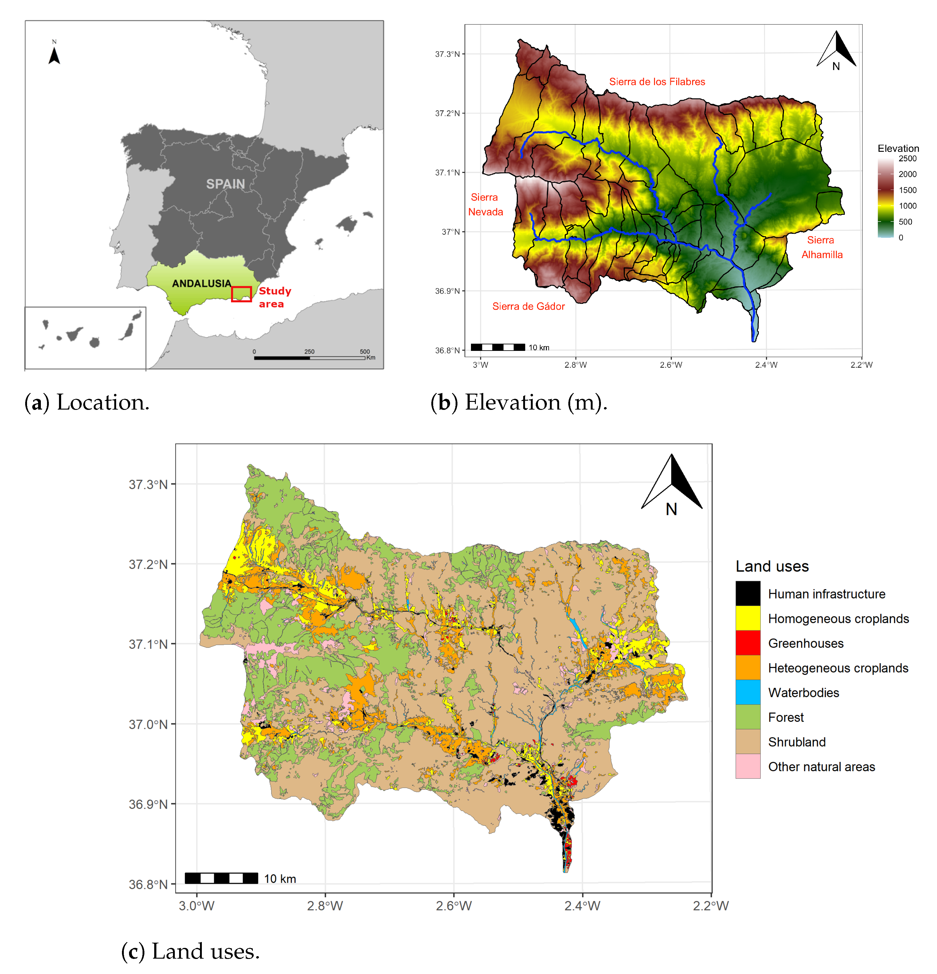
2.1. Study Area

The study area is the Andarax catchment, a region in the south-easternmost part of Andalusia (Spain) that covers an area of 598 km${}^2$ (Figure 1). It borders with Sierra de los Filabres in the North, Sierra Nevada in the West, Sierra de Gádor in the Southwest and Sierra Alhamilla in the Southeast. The Andarax river arises in the easternmost part of Sierra Nevada, joins its main tributary (the Nacimiento river) in its middle course and, finally, flows into the Mediterranean Sea.

The altitude of the study area ranges from 0 to 2500 m above the sea level. Its orographic diversity enables a wide variation in volume of rainfall and temperature, with rainier and colder areas being located in the mountain ranges, whereas drier and hotter regions lie on the inner depressions among the ranges. Thus, the climatic conditions determine a wide variety of landscapes, from alpine (Sierra Nevada) to semi-arid (Tabernas desert), with fuzzy transitions between them in some cases.

Concerning the land-use and land cover, natural vegetation is predominant, with more than 50% of the study area being occupied by shrubland and more than 20% by forest. On the one hand, large areas of pine trees (Pinus sp.) and some relict areas of Mediterranean forest with oak are found in the slopes of the mountain ranges, whereas more than 40 different species of shrub occupy lower areas, with esparto grass (Stipa tenacissima) being the most frequent one. On the other hand, plains located along the rivers and streams are mainly used as croplands.

Regarding the socio-economy, the catchment is occupied by 51 municipalities, with those located at low altitudes boasting greater wealth and higher levels of education, as well as greater work opportunities and higher immigration rate. By contrast, municipalities in the high mountains are characterized by depopulation and aging population.

2.2. Data Collection and Preprocessing

The dataset comprises a set of social, economic and environmental variables selected according to literature and expert knowledge [32]. Two different sources of information were used: the Andalusian Environmental Information Network provided the environmental information (retrieved 10 October 2014, from http://www.juntadeandalucia.es/medioambiente/site/rediam), while the Andalusian Institute of Statistics and Cartography provided social and economic data (retrieved 19 October 2014, from http://www.juntadeandalucia.es/institutodeestadisticaycartografia/sima/index2-en.htm) per municipality (

Table A1. Description of the land-related variables.

Group	Variable	Definition	Range
Land use	Forest land	% of land occupied by forest trees or pastures, sometimes combined with shrubs	0 = [0, 11] (n = 768) 1 = (11, 52] (n = 770) 2 = (52, 100] (n = 768)
Land use	Homogeneous cropland	% of land occupied by herbaceous or woody monocultures	0 = 0 (n = 1299) 1 = (0, 15] (n = 505) 2 = (15, 100] (n = 502)
Land use	Heterogeneous cropland	% of the land occupied by mixtures of herbaceous and woody crops or mixtures of crops and natural vegetation	0 = 0 (n = 1538) 1 = (0, 7] (n = 385) 2 = (7, 100] (n = 383)
Land use	Shrubland	% of land occupied by shrubs with absence of trees	0 = [0, 11] (n = 768) 1 = (11, 63] (n = 768) 2 = (63, 100] (n = 770)
Land use	Human infrastructure	% of urban, industrial and commercial areas, landfills, mining deposits and communication infrastructures	0 = 0 (n = 1851) 1 = (0, 5] (n = 228) 2 = (5, 100] (n = 227)
Land use	Greenhouse	% of high yield irrigated crops under controlled conditions	0 = 0 (n = 2158) 1 = (0, 2] (n = 75) 2 = (2,100] (n = 73)
Soil	Cambisols	% of cambisols	0 = 0 (n = 1092) 1 = (0, 99] (n = 361) 2 = (99, 100] (n = 853)
Soil	Fluvisols	% of fluvisols	0 = 0 (n = 1867) 1 = (0, 57] (n = 220) 2 = (57, 100] (n = 219)
Soil	Lithosols	% of lithosols	0 = 0 (n = 1809) 1 = (0, 99] (n = 228) 2 = (99, 100] (n = 269)
Soil	Luvisols	% of luvisols	0 = 0 (n = 2182) 1 = (0, 45] (n = 63) 2 = (45, 100] (n = 61)
Soil	Regosols	% of regosols	0 = 0 (n = 1719) 1 = (0, 88] (n = 294) 2 = (88, 100] (n = 293)
Soil	Xerosols	% of xerosols	0 = 0 (n = 2008) 1 = (0, 76] (n = 150) 2 = (76, 100] (n = 148)
Geomorphology	Anthropic	% of anthropic geomorphological type	0 = 0 (n = 2284) 1 = (0, 9] (n = 12) 2 = (9, 45] (n = 10)
Geomorphology	Gravitational	% of gravitational geomorphological type	0 = 0 (n = 1921) 1 = (0, 29] (n = 193) 2 = (29, 100] (n = 192)
Geomorphology	Denudational	% of denudational geomorphological type	0 = 0 (n = 1674) 1 = (0, 64] (n = 317) 2 = (64, 100] (n = 315)
Geomorphology	Structural	% of structural geomorphological type	0 = 0 (n = 830) 1 = (0, 99] (n = 740) 2 = (99, 100] (n = 736)
Geomorphology	Fluvial	% of fluvial geomorphological type	0 = 0 (n = 1598) 1 = (0, 23] (n = 355) 2 = (23, 100] (n = 353)
Geomorphology	Glacial	% of glacial geomorphological type	0 = 0 (n = 2264) 1 = (0, 53] (n = 22) 2 = (53, 100] (n = 20)
Geomorphology	Karst	% of karst geomorphological type	0 = 0 (n = 1666) 1 = (0, 74] (n = 321) 2 = (74, 100] (n = 319)
Lithology	Metamorphic	% of metamorphic rock	0 = [0, 55] (n = 769) 1 = (55, 99] (n = 258) 2 = (99, 100] (n = 1279)
Lithology	Sedimentary	% of sedimentary rock	0 = 0 (n = 1286) 1 = (0, 99] (n = 482) 2 = (99, 100] (n = 538)
Lithology	Plutonic	% of plutonic rock	0 = 0 (n = 2299) 1 = (0, 12] (n = 4) 2 = (12, 83] (n = 3)

and

Table A2. Description of the socio-economic and climatic variables.

Group	Variable	Definition	Range
Social	Population natural growth	Growth of the population, computed as the difference between the number of births and deaths	[−25, 782]
Social	Aging	% of people older than 65 years	[6.73, 48.91]
Social	No studies	% of people who do not have any level of educational attainment, including illiterates (computed from people over 16)	[2.67, 72.06]
Social	Primary studies	% people whose maximum level of education attained is elementary school (computed from people over 16)	[4.51, 49.25]
Social	Secondary studies	% people whose maximum level of education attained is high school (computed from people over 16)	[16.18, 56.59]
Social	Tertiary studies	% people whose maximum level of education attained is a university degree (computed from people over 16)	[1.63, 16.33]
Social	Emigration	% of emigrants	[1.37, 21.45]
Social	Immigration	% of immigrants	[1.42, 15.33]
Economic	Income per capita	Average net income declared ()	[5178, 18184]
Economic	Unemployment	% of workforce that is unemployed	[3.97, 43.48]
Economic	Primary sector employment	% of people working in the primary sector	[0, 59.5]
Economic	Secondary sector employment	% of people working in the secondary sector	[7.69, 43.95]
Economic	Tertiary sector employment	% of people working in the tertiary sector	[0, 26.92]
Climate	Coldest month temperature,	Minimum temperature of the averages of the minimum monthly temperatures (°C) over the period 1961–2000	[0.7, 12.58]
Climate	Annual temperature	Average annual mean temperature (°C) over the period 1961–2000	[7.32, 18.93]
Climate	Spring rainfall	Average spring total rainfall (mm) over the period 1961–2000	[16.94, 56.56]
Climate	Summer rainfall	Average summer total rainfall (mm) over the period 1961–2000	[3.32, 14.37]
Climate	Annual rainfall	Average annual total rainfall (mm) over the period 1961–2000	[172, 639.49]
Climate	Annual number of rainfall days	Average number of annual rainy days over the period 1961–2000	[8.21, 26.65]
Climate	Spring number of rainfall days	Average number of vernal rainy days over the period 1961–2000	[2.08, 5.38]
Climate	Summer number of rainfall days	Average number of estival rainy days over the period 1961–2000	[1.48, 6.12]
Climate	Evapotranspiration rate	Average annual evapotranspiration of reference (mm) over the period 1961–2000	[541.99, 951.20]

, in Appendix A).

In order to keep the number of variables relatively low, the basic levels of categorization were used for the ground-related variables, i.e., land-use, soil, geomorphology and lithology variables (Table A1). Moreover, these variables were discretized into 3 intervals with equal frequency to avoid problems related to zero-inflation. In the cases of extremely high concentration of values at 0, the discretization into equal frequency bins was carried out for the non-zero values, so that all zero values fall into the first interval.

All variables were expressed at the 1 km${}^2$ grid scale. In the case of the environmental variables, the information was rasterized (if needed) and their averages were computed for each grid cell. On the other hand, the socio-economic variables were originally expressed at the municipality scale, therefore they had to be computed at the grid scale. In particular, grid cells falling inside a single municipality take the municipal values for the socioeconomic variables, whereas grid cells falling between two or more municipalities take the weighted mean of the socio-economic variable, calculated according to the percentage of grid cell occupied by each municipality included in the cell. In this way all the information was expressed using the same 1 × 1 km grid. Finally, the complete dataset was composed of 44 variables (22 discretized) taking values over 23,061 km${}^2$ cells.

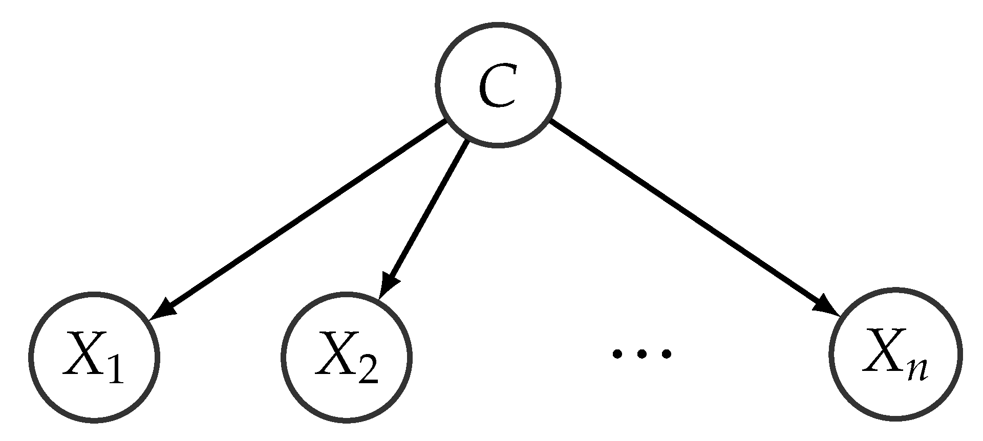
2.3. Hybrid Bayesian Networks

A Bayesian network [24] is a statistical multivariate model for a set of variables $\mathbf{X}=\{X_1,\cdots ,X_n\}$, whose independence relations are encoded by the structure of an underlying Directed Acyclic Graph (DAG). More specifically, the DAG is composed of nodes that represent random variables (X) and links between pairs of nodes, representing statistical dependence between them. Each node $X_i$ has a conditional probability distribution $p\left(x_i\right|pa\left(x_i\right))$ attached, where $pa\left(x_i\right)$ represents the parents of $X_i$ in the DAG.

The main advantage of BNs is that the DAG structure provides information about the relationships between variables and makes it possible to identify which variables are relevant (or irrelevant) for some other variable of interest, based on the d-separation concept [24]. This allows us to simplify the Joint Probability Distribution (JPD) of the variables necessary to specify the model. Thus, BNs provide a compact representation of the JPD over all variables, defined as the product of the conditional distributions attached to each node, so that:

$$p(x_1,\dots ,x_n)=\prod _{i=1}^{n}p(x_i\mid pa\left(x_i\right)).$$

(1)

where $pa\left(x_i\right)$ is the set of parents of variable $x_i$ according to the DAG.

A hybrid BN is a BN that contains both discrete and continuous variables simultaneously. Dealing with hybrid data is not an easy task and various solutions have been proposed. In this paper, the Mixture of Truncated Exponential model (MTE) [33] has been applied. This solution proposes to divide the support of a continuous variable into several intervals and approximate its probability density within the interval by an exponential function, rather than by a constant, unlike in discretization methods. As a result, the more intervals used to divide the domain of the continuous variables, the higher the accuracy of the MTE model, but also its complexity, in terms of number of parameters. On the other hand, unlike conditional linear Gaussian Bayesian networks, MTEs do not impose restrictions on the model structure and are able to approximate any kind of distribution thanks to its high fitting power. More details about MTE models can be found in [34,35,36].

2.4. Unsupervised Classification Using Hybrid BNs

BNs have been successfully used for classification tasks. The simplest BN classifier is the Naive Bayes (NB) [37], a fixed structure whose class variable C is the the parent of all remaining variables $X_1,\cdots ,X_n$, and these are considered independent of each other given C (Figure 2). This strong independence assumption is compensated by the reduction in the number of parameters to be estimated from data, since in this case, it holds that:

$$p(c\mid x_1,\dots ,x_n)\propto p\left(c\right)\prod _{i=1}^{n}p(x_i\mid c),$$

(2)

which means that, instead of one n-dimensional conditional distribution, n one-dimensional conditional distributions are estimated. Despite this extreme independence assumption, the results are highly accurate in many cases, and for this reason, it has become a widespread Bayesian network classifier in the literature.

Classification tasks can be divided into two broad categories: supervised and unsupervised. Supervised classification consists in predicting the value of a discrete variable of interest, called the class C, given the values of a set of predictive or feature variables, $X_1,\cdots ,X_n$. In other words, given a class variable C, with k possible values, the goal of a supervised classifier is to obtain the probability that an object with observed features $x_1,\cdots ,x_n$ belongs to each class $C=c_k$ and returns the most likely one.

On the other hand, unsupervised classification [21] is performed taking into account that no information about class variable C is given. In this regard, the goal of an unsupervised classifier is to find groups of elements based on their similarities. In this work, we follow the methodology proposed in [31,38] (Algorithm 1), which details the specific steps and algorithms, implemented in Elvira software [39]. In this approach, the class variable C is replaced by a hidden variable, H, whose values are initially missing. H is included in the dataset to represent the membership of each case to the different clusters. In the first step, an initial model is learned with 2 clusters ($k=2$ for variable H) and the a priori probability distribution for H is defined as uniform (Algorithm 2). Using the data augmentation method [40] the initial model is refined to return the 2-clusters model with higher likelihood. This algorithm is an iterative procedure, similar to the Expectation Maximization algorithm [41], in which (i) the values for the H variable are simulated for each case in the dataset according to the probability distribution for H; (ii) the parameters of the probability distribution of the variables in the model are re-estimated according to the new simulated data. This process is repeated until no improvement in likelihood is achieved. During this iterative process a validation is carried out by dynamically dividing the dataset into training and test sets (Algorithm 3). Once the best model for two clusters is obtained, the next step is to add a new cluster (Algorithm 4), by splitting one of the existing ones into two (increasing the number of states of variable H), and to perform the data augmentation again to optimize the parameters. If this new model improves the previous one in terms of likelihood it is accepted, and the process is repeated until the likelihood value of the model with k clusters does not improve with respect to the previous one. In that case, $k-1$ is the optimal number of clusters.

In this study, an unsupervised classification based on hybrid BNs with NB structure was carried out, where the class is a hidden variable, H, that represents the socio-ecological sectors, and the features are the remaining 44 variables (Table A1 and Table A2). As a result, the classifier returns the probability of each observation (grid cell) belonging to each socio-ecological sector. This is in contrast with the so-called hard clustering methods like k-means and hierarchical clustering, which yield rules that assign each individual to a single group, therefore producing classes with sharp bounds.

Algorithm 1: Probabilistic clustering based on hybrid Bayesian networks for the landscape data set.

Algorithm 2: LearnInitialModel.

Another advantage of the model that we use in this work (i.e., NB with MTE distributions) with respect to its natural competitor (NB with Gaussian distributions estimated using the EM algorithm) is that the resulting number of clusters is significantly lower for similar goodness of fit [38]. It means that the risk of spurious divisions between the socio-ecological sectors found is lower.

Algorithm 3: DataAugmentation.

Algorithm 4: AddCluster.

Input: A model $M_0$ with n states in the hidden variable $H_0$.    Output: A new model M with $n+1$ states in the hidden variable H. 1 $M\leftarrow M_0$. 2 Let $h_1,\dots ,h_n$ be the states of the hidden variable H in M. 3 Add a new state, $h_{n+1}$ to H. 4 Update the probability distribution of H by re-computing the probability of $h_n$       and $h_{n+1}$ as follows: 5       $a\leftarrow p\left(h_n\right)/2$. 6     $p\left(h_n\right)\leftarrow a$. 7 $p\left(h_{n+1}\right)\leftarrow a$. 8 foreach feature $X_i$ in M do 9 10 return M.

2.5. Boundary Detection

In spatial analysis, clustering or unsupervised classification means dividing the territory into several sectors whose members share common characteristics [21]. Following the methodology explained above, the model returns the probability of any grid cell belonging to each sector. Two possible approaches can be followed to determine which sector an observation belongs to: (i) the hard clustering approach, i.e., classify each observation into the sector with the highest probability value or (ii) the soft clustering approach, i.e., specify a minimum probability value to classify an observation as belonging to a sector; if no sector surpasses the threshold, the observation is classified as a boundary zone.

Table 1. An example of the results obtained from the model, in which the probability of belonging to each of three sectors (P(H = h), with $h=1,2,3$) is presented. Max. Prob. refers to a classification based on the highest probability value. In contrast, the last column shows the probability threshold method for $t=0.8$.

Grid Cell	P($\mathit{H}=1$)	P($\mathit{H}=2$)	P($\mathit{H}=3$)	Max. Prob.	$\mathit{t}=0.8$
1	0.5	0.25	0.25	1	Boundary
2	0.05	0.13	0.82	3	3
...	...	...	...	...	...
2306	0.71	0.18	0.11	1	Boundary

shows an example of the results obtained from the model using each approach. If the first one is followed, each grid cell is classified as belonging to the sector h with highest probability. In the example, the grid cell 1 is classified into Sector 1, with $P(H=1)=0.5$, and the grid cell 2 into Sector 3, with $P(H=3)=0.82$. In this way, no boundary zones are detected since all the observations are assigned to a sector. On the other hand, the second approach allows to identify observations that do not clearly belong to any sector. In the example, for a threshold value $t=0.8$, the grid cell 1 is now classified as boundary, whilst the grid cell 2 is still assigned to Sector 3.

Our proposal follows the second approach by setting a probability threshold, t, so that an observation with $P(H=h)\ge t$ will be classified as belonging to sector h (with $h=1,\cdots ,k-1$). If this condition is not fulfilled for any sector, the observation will be classified as a boundary zone. In other words, boundary zones are not similar enough to the elements of any sector and, thus, they do not belong to any of them. Note that the number of grid cells classified as boundary zones depends on the value chosen for t, i.e., the higher the value t is, the higher the number of boundary cells obtained.

In this paper, different thresholds, t = {$0.70$, $0.75$, $0.80$, $0.85$, $0.90$, $0.95$} were adopted for boundary detection. Afterwards, the boundaries obtained were grouped in zones, according to the sectors they split. To identify whether or not these zones behave as boundaries, the Wilcoxon rank-sum hypothesis test was used to compare the boundary zone to each of the sector it separates. The original (non-discretized) data was used to perform the hypothesis tests.

3. Results and Discussion

The methodology applied yielded six socio-ecological sectors. The characteristics of each sector will be described in Section 3.1 and the boundaries found will be analyzed in Section 3.2.

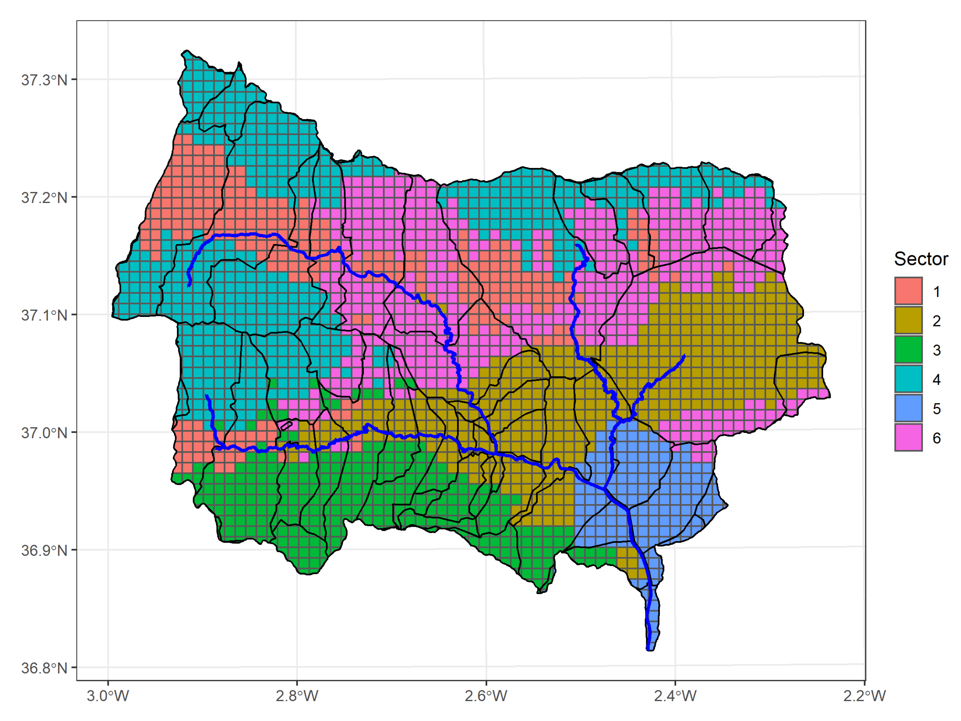
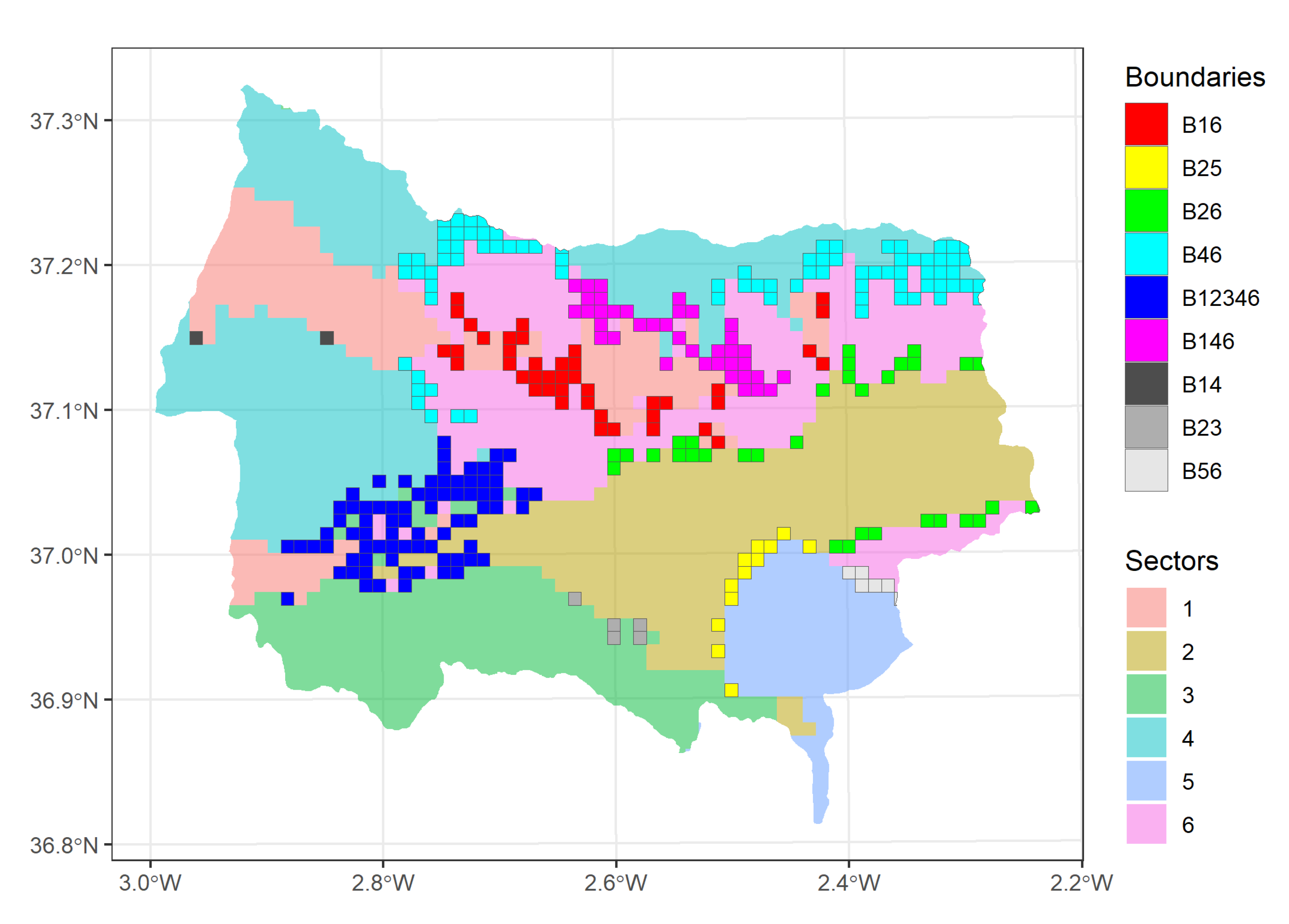
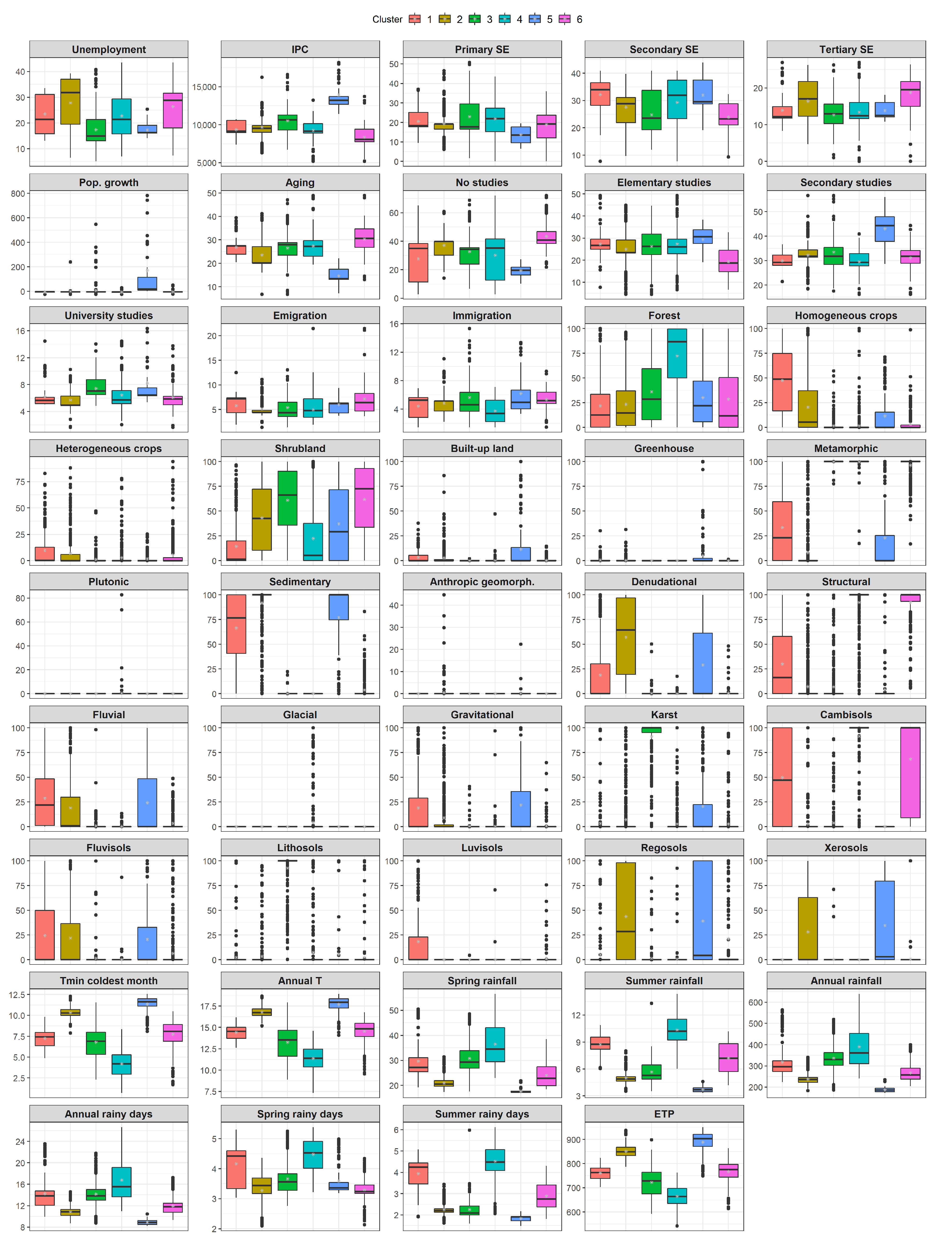
3.1. Socio-Ecological Sectors

Figure 3 shows the identified socio-ecological sectors, where each observation is classified into the sector that returns the highest probability, i.e., no threshold is applied to find boundaries. A spatial longitudinal pattern from the upper to the lower river course was found, as well as an altitudinal gradient from the riverbed to the mountain peaks. The defining characteristics of each sector are outlined below, with the mean values of the most relevant variables, in standardized scores:

• Sector 1 comprises grid cells located at the upper river courses. This cluster is characterized by a high percentage of homogeneous crops ($z=1.45$, i.e., it is 1.45 standard deviations above the mean, on average) and high percentage of luvisols ($z=1.19$). The presence of shrubland is scarce in this region ($z=-0.7$), occupying less than 15% of the sector.
• Sector 2 comprises inner lowland grid cells, characterized by the predominance of the sedimentary material, which occupies more than 90% of the sector ($z=1.27$). Furthermore, the annual temperature, the minimum temperature of the coldest month and the evapotranspiration (ETP) take higher-than-average values ($z>1$). In this sector shrubs and homogeneous crops (mainly extensive areas of olive crops) coexist.
• Sector 3 comprises grid cells located in Sierra de Gádor, the southernmost mountain range on the study area. This sector is characterized by a high percentage of karst landscape ($z=2.02$) and high percentage of lithosols ($z=2.05$). In terms of land-use, this sector presents the lowest percentage of land occupied by both heterogeneous and homogeneous crops (≤3%).
• Sector 4 comprises grid cells located in the uppermost parts of Sierra Nevada and Sierra de los Filabres. This sector is characterized by low temperatures (both, annual and minimum of coldest month, with $z<-1$) and ETP ($z=-1.13$), and high rainfall, especially summer rainfall and summer rainy days ($z>1$). In terms of land-uses, this sector presents the highest percentage of land occupied by forest (>72%) in comparison with the remaining sectors ($z=0.93$).
• Sector 5 comprises grid cells at the lowest elevation and is mainly characterized by the socio-economic and climatic variables. More specifically, the Income Per Capita (IPC) is two standard deviations above the mean; moreover, the population growth is higher than in the remaining sectors ($z=1.62$) whereas the proportion of population over 65 years old is lower ($z<-1.5$). Regarding the climatic variables, this sector shows high temperatures and ETP ($z>1$) and low amount of rainfall and rainy days ($z<-1$).
• Sector 6 is mainly located at the foothills of Sierra de los Filabres, Sierra Nevada and Sierra Alhamilla. This sector is characterized by a population with lower IPC ($z=-0.69$), higher proportion of older people ($z=0.62$) and higher emigration rate ($z=0.6$).

The distribution of the socio-ecological variables in each sector can be seen in Figure A1 in Appendix B. The mean z-score of some relevant socio-ecological variables are shown in

Table 2. Mean standardized scores of some socio-ecological variables by sector. For each variable, the highest mean is shown in green and the lowest in red.

Variable	Sector 1	Sector 2	Sector 3	Sector 4	Sector 5	Sector 6
IPC	−0.2	−0.04	0.37	−0.25	2.05	−0.69
Primary SE	0.05	−0.09	0.34	0.21	−0.77	−0.16
Aging	0.14	−0.33	0.09	0.21	−1.57	0.62
No studies	−0.38	0.27	−0.04	−0.21	−0.96	0.7
Emigration	0.05	−0.2	−0.1	−0.28	0.14	0.6
Forest	−0.47	−0.43	−0.08	0.93	−0.24	−0.29
Homogeneous crops	1.45	0.33	−0.44	−0.44	−0.04	−0.37
Heterogeneous crops	0.41	0.18	−0.29	−0.16	−0.23	0.06
Annual temperature	0.06	1.01	−0.41	−1.17	1.37	0.11
Annual rainfall	0.18	−0.68	0.36	0.94	−1.21	−0.37

.

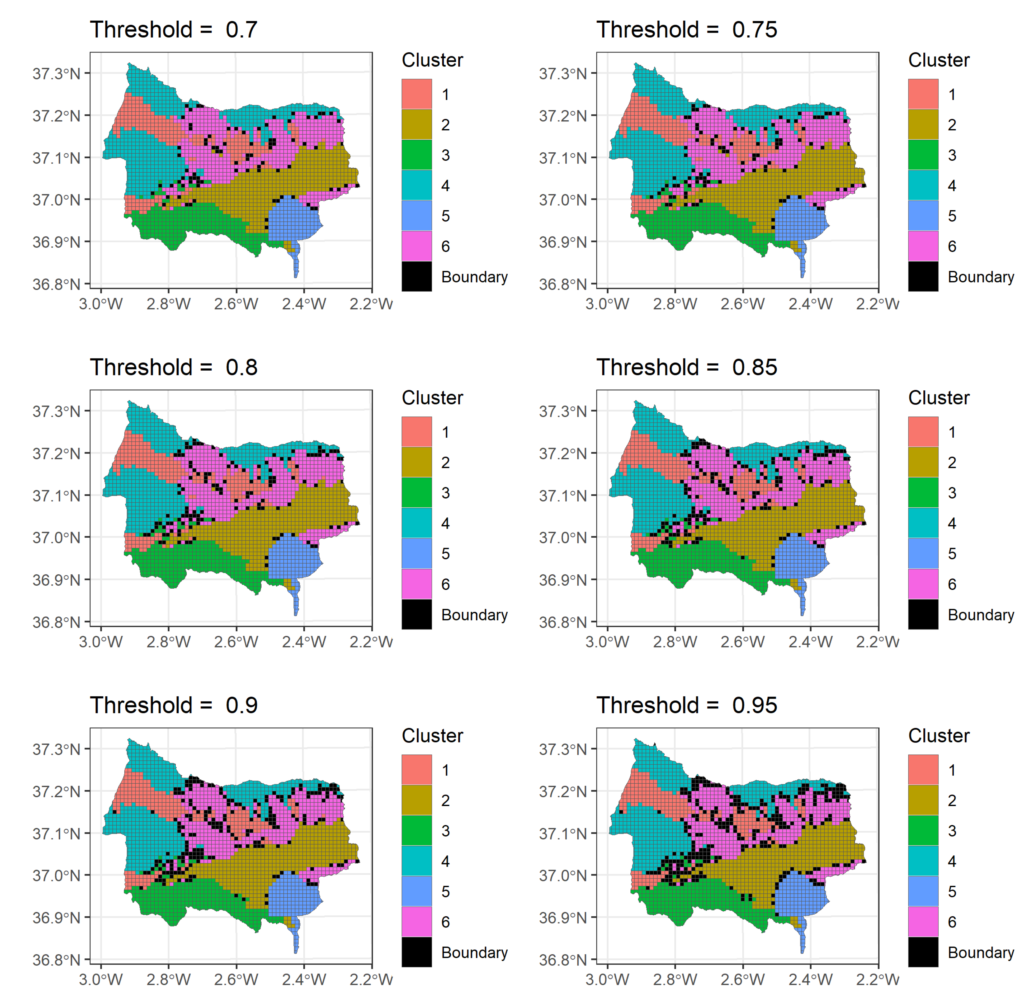
3.2. Socio-Ecological Boundary Areas

Figure 4 shows the boundary zones found using different thresholds, t = {$0.70$, $0.75$, $0.80$, $0.85$, $0.90$, $0.95$}. The boundary zones are already visible from the lowest threshold ($t=0.7$), and they get thicker as the threshold gets higher, i.e., as t increases, so does the size of the boundary area. This is due to adding additional observations to the ones previously classified as boundary. Further analyses were performed for the boundaries found with $t=0.95$, as they are larger.

Figure 5 shows the boundary areas classified in groups according to the sectors they separate. The boundary zones have been named after the sectors they split, for instance, $B16$ refers to the boundary area that is in between Sectors 1 and 6. Figure A2, Figure A3, Figure A4, Figure A5, Figure A6 and Figure A7 show the boxplots of the socio-ecological variables within each boundary zone and their adjacent sectors, indicating whether or not significant differences are found between them. The description of each boundary zone is presented below.

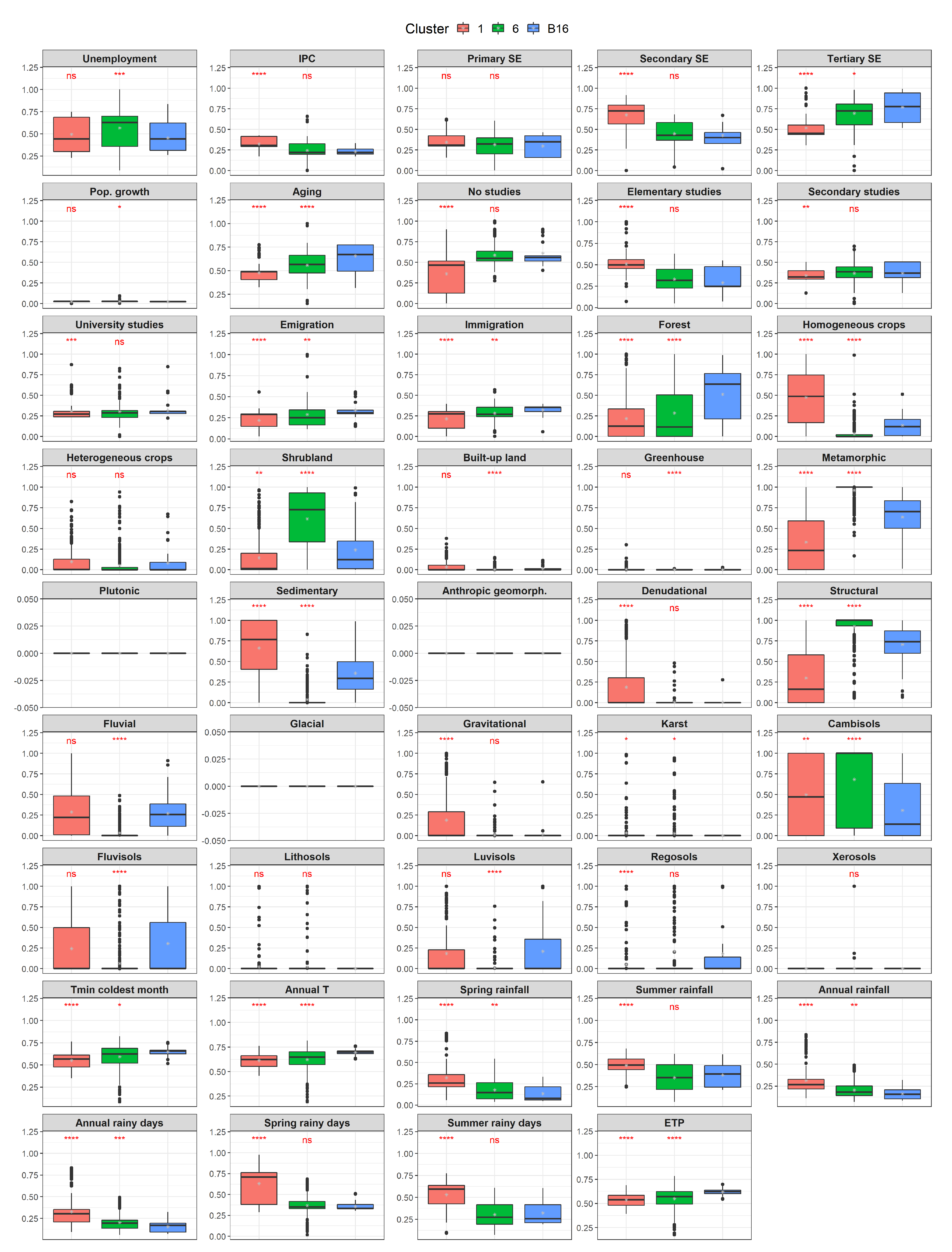
• $B16$: This boundary zone separates Sectors 1 (upper river area) and 6 (foothills) and is mainly located along the middle course of the Nacimiento river, at a lower elevation than the other two sectors. From the socio-economic point of view, the boundary zone seems to be more similar to Sector 6 than 1, as the medians of most variables are closer and no statistically significant differences are found in many cases (Figure A2). In terms of lithology, while Sector 1 is predominantly sedimentary and Sector 6 is metamorphic, the boundary zone is mixed, showing statistically significant differences with both sectors. Concerning land-uses, Sector 1 is largely covered by herbaceous crops and Sector 6 by shrubland. However, the boundary zone is predominantly covered by forest, showing statistically significant differences with both sectors. Finally, regarding the climate variables, the lower elevation at which the boundary zone is located determines its hotter and drier conditions, with the hypothesis test performed yielding significant differences between the boundary and both sectors, in most cases.
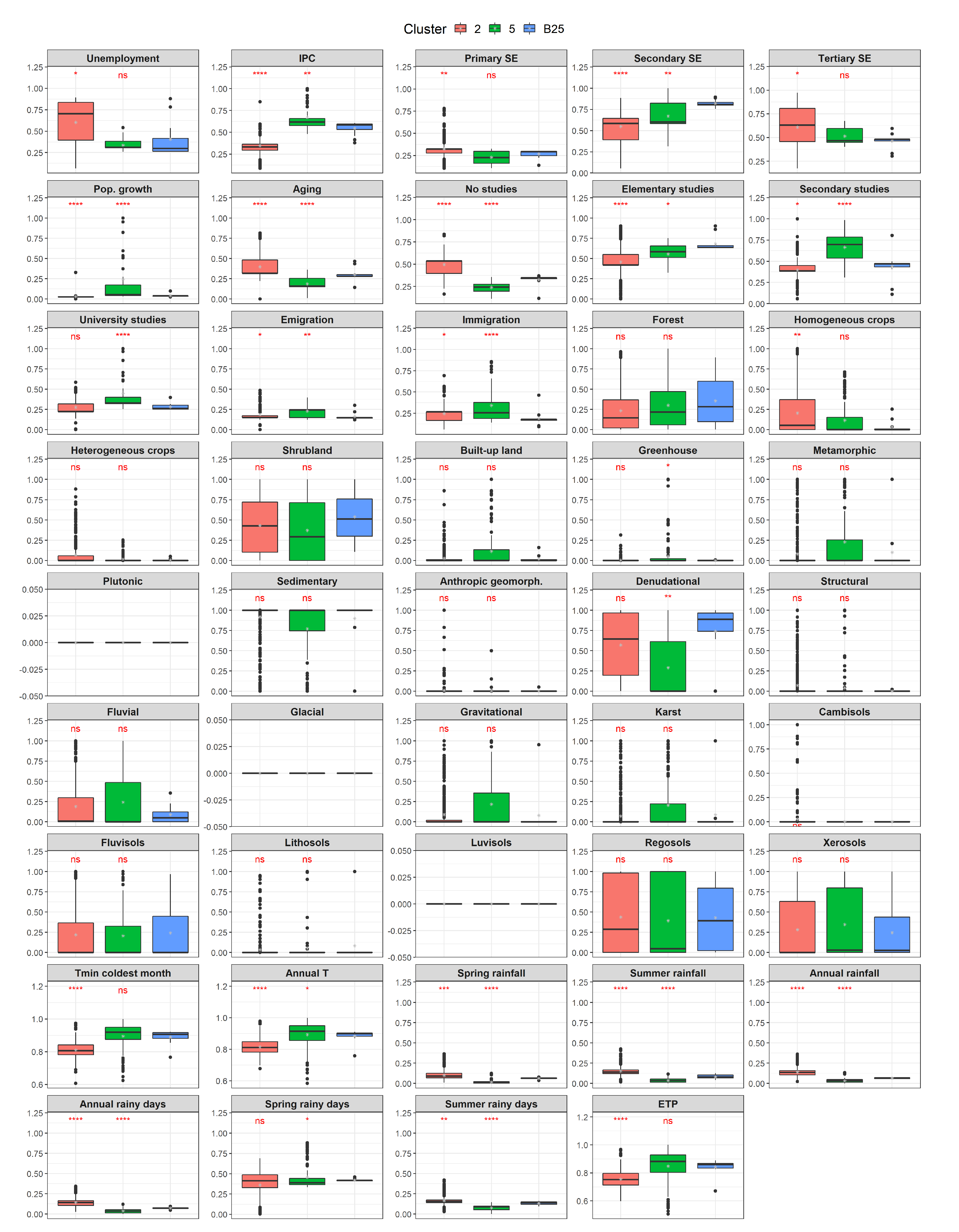
• $B25$: This boundary zone divides Sectors 2 (inner lowlands) and 5 (wealthier land). In general, the statistical test yielded significant differences regarding the socio-economic and climate variables (Figure A3). In terms of the economic variables (unemployment, IPC and sector employment), the boundary zone is more similar to Sector 5 than 2. Regarding the remaining social and climate variables, the boundary zone takes intermediate values between the two sectors, yielding statistically significant differences, in most cases.
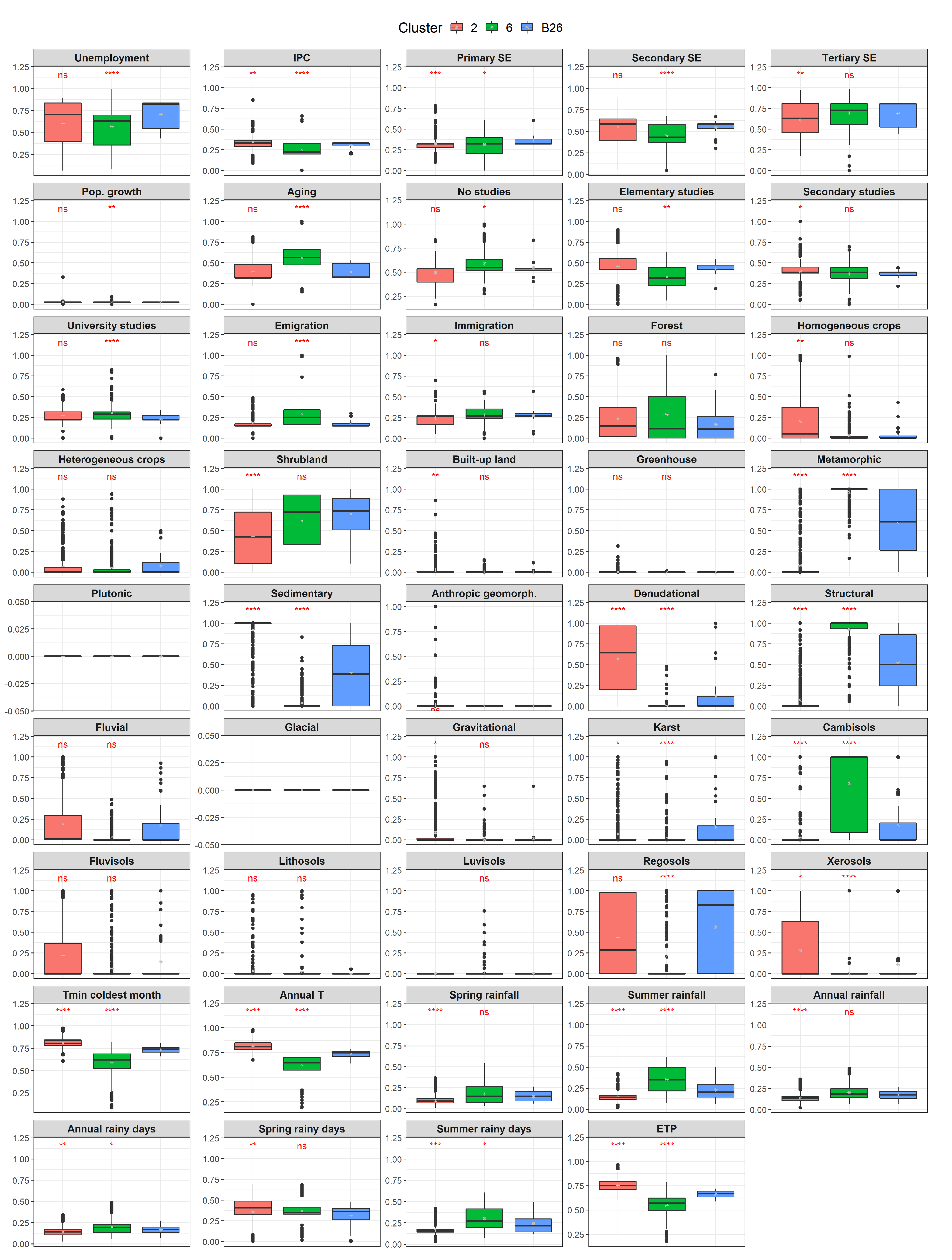
• $B26$: This boundary zone divides Sectors 2 (inner lowlands) and 6 (foothills). The transition in altitude is reflected in the climatic conditions of the boundary area, as it shows intermediate values between both sectors, showing statistically significant differences between the boundary zone and each sector, in most cases (Figure A4). In terms of land-uses, significant differences were not found between the boundary zone and Sector 6, whereas Sector 2 and the boundary zone present significant differences regarding, homogeneous crops, shrubland and built-up land. Regarding the socio-economic variables, significant differences were found between the boundary zone and Sector 2 in five out of 13 variables and between the boundary area and Sector 6 in 10 out of 13 variables. Therefore, this boundary zone is more similar to Sector 2 from the socio-economic point of view and more similar to Sector 6 from the land-use point of view, but with warmer and drier climate conditions.
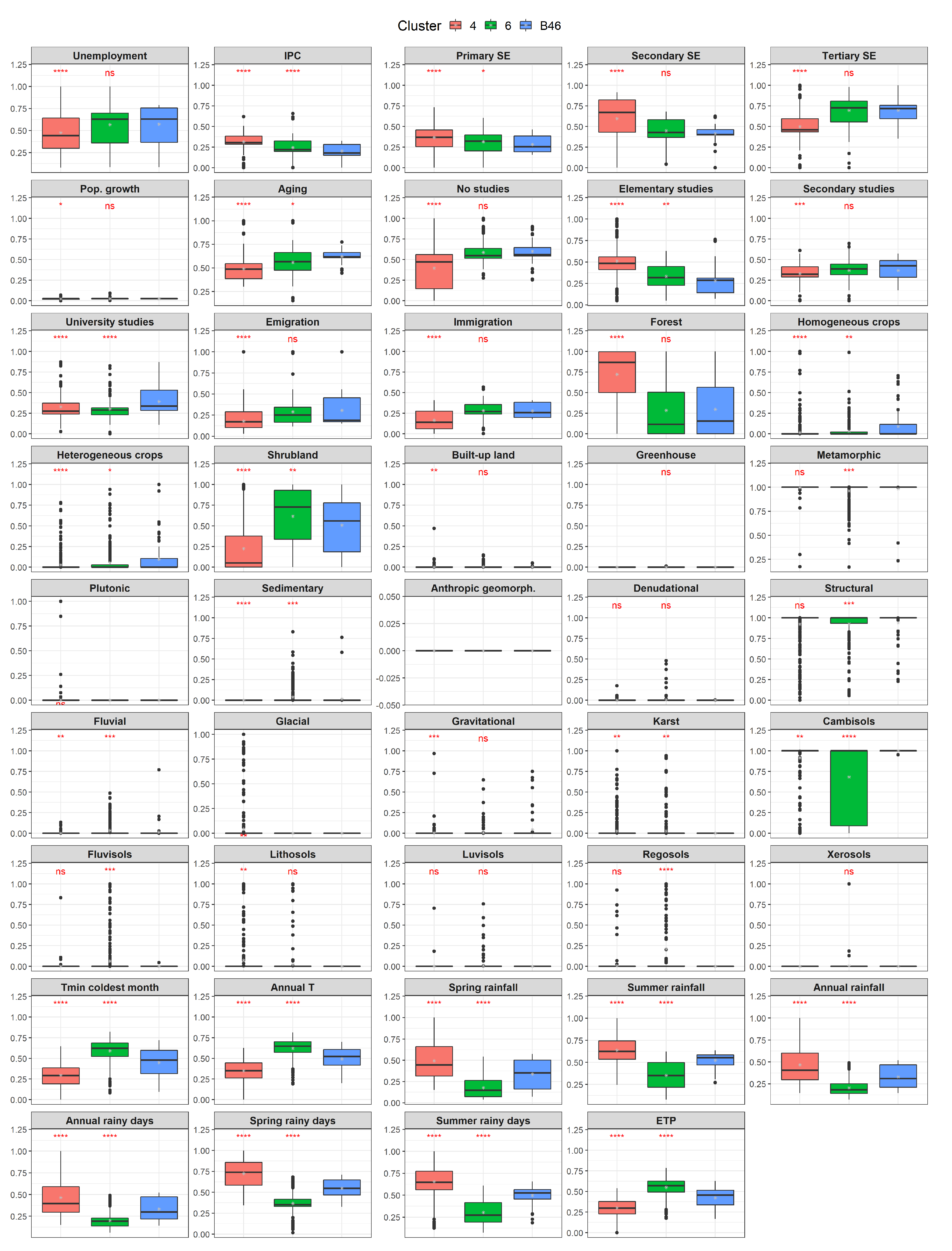
• $B46$: This boundary zone is located between Sectors 4 (high mountain) and 6 (foothills). As occurred in boundary $B26$, the transition in altitude causes a shift in the climate variables, with the boundary zone taking intermediate values with respect to the two sectors (Figure A5). Regarding land-uses, the boundary zone shows differences with the two sectors, presenting a higher coverage of homogeneous and heterogeneous crops, a coverage of forest similar to Sector 6 and a coverage of shrubland intermediate between the two sectors. Concerning the socio-economic variables, significant differences were found between the boundary zone and Sector 4 in all variables and between the boundary zone and Sector 6 in five out of 13 variables.
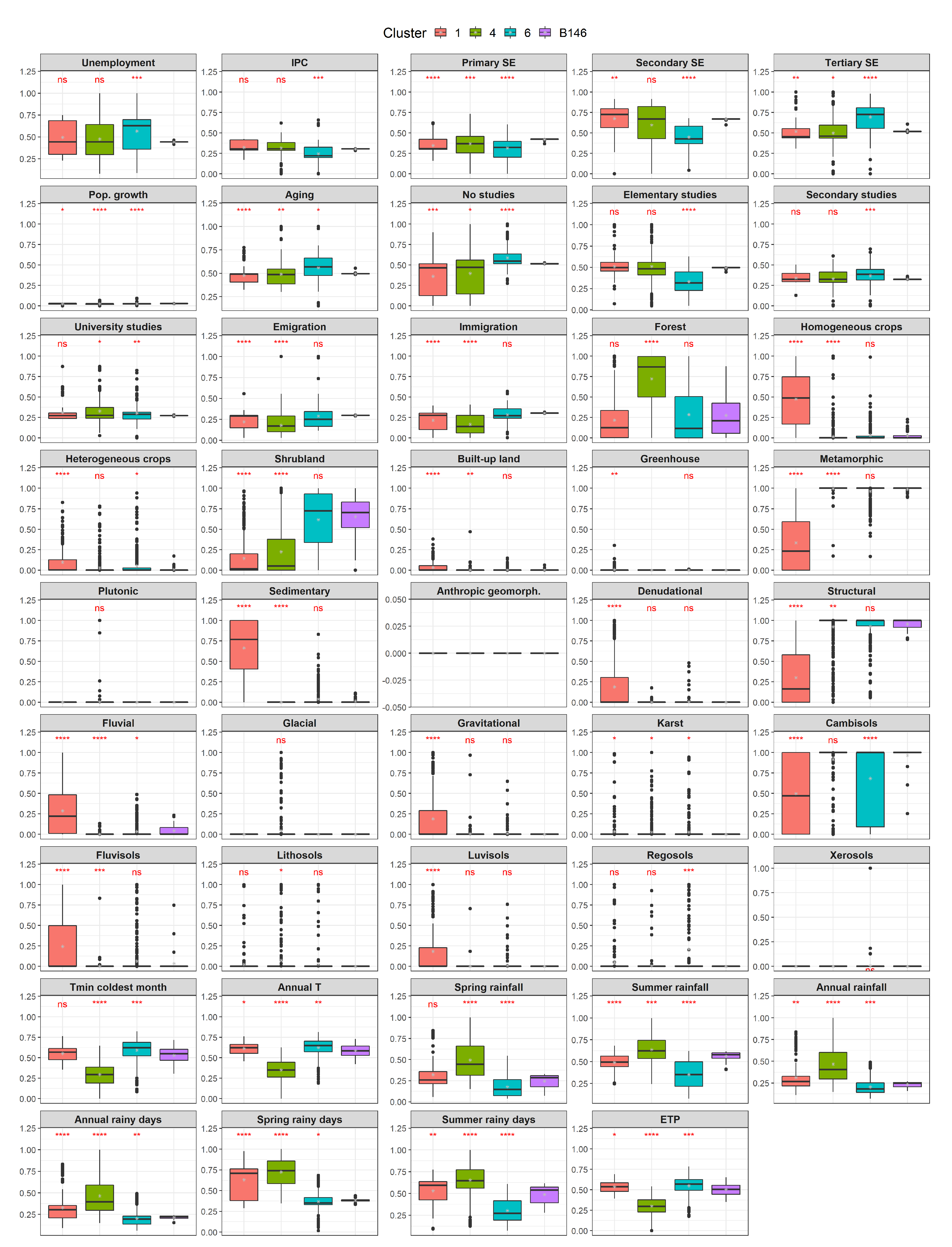
• $B146$: This boundary zone divides Sectors 1 (upper river courses), 4 (high mountains) and 6 (foothills). From the socio-economic point of view, it completely lies within one municipality, and therefore, the values of these variables in this zone hardly vary (Figure A6). Regarding land-uses, this boundary is more similar to Sector 6, due to its dominance of shrubland, and shows significant differences with the other two sectors in most variables. Concerning the climate variables, the boundary zone takes intermediate values between Sectors 4 and 6, with the statistical test yielding significant differences in all cases.
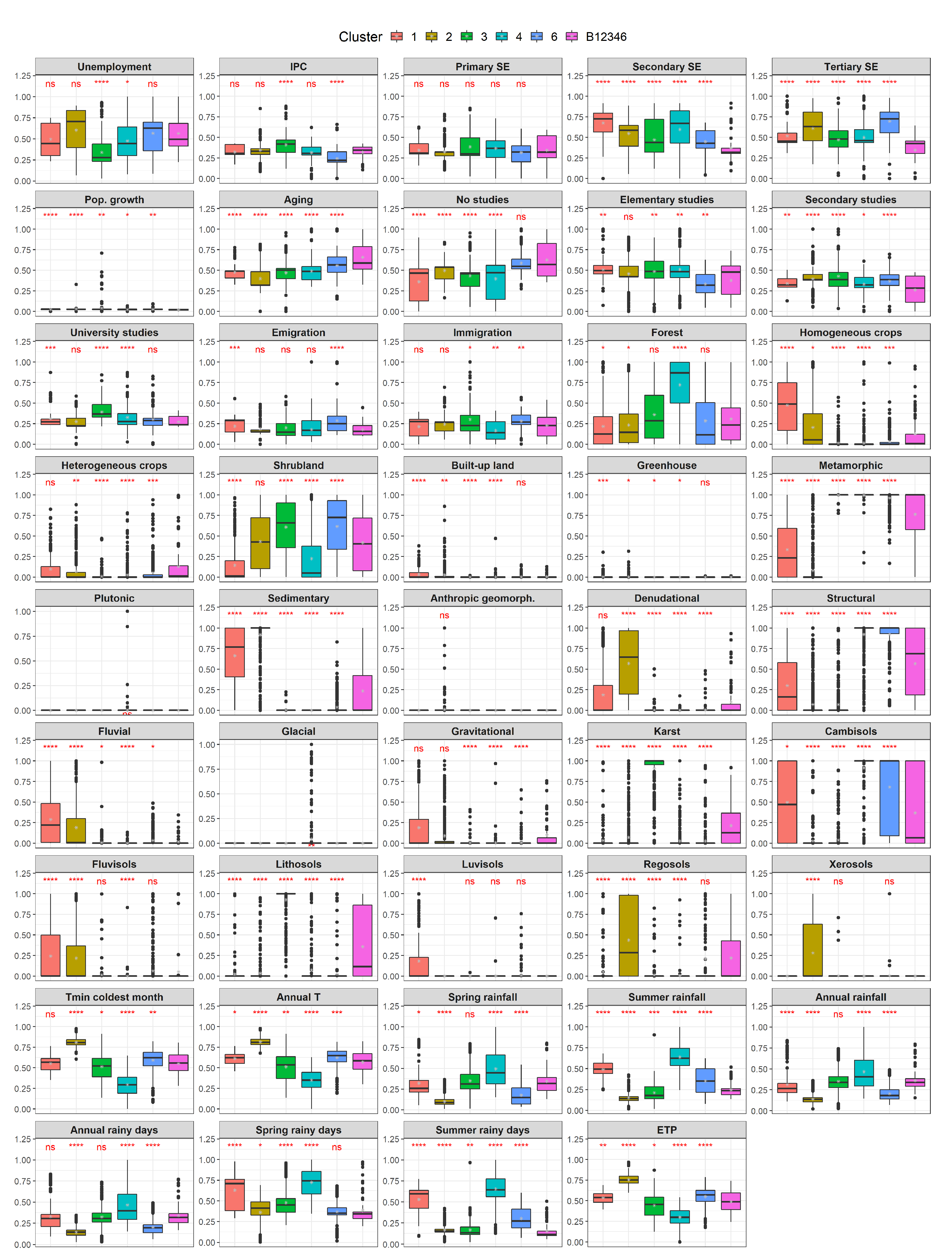
• $B12346$: Finally, this boundary zone is a highly heterogeneous a complex area that divides a total of five sectors. It is located between two mountain ranges, Sierra de Gádor and Sierra Nevada, and covers part of the middle course of the main river of the catchment (Figure A7).

Our results show a set of grid cells classified as boundaries according to the probabilistic threshold $0.95$, but maps with other thresholds can also be obtained (Figure 4). The catchment studied is a cultural landscape (a socio-ecological system) that can be considered a nested system, so it can be studied and analyzed from local to regional to global scales [42]. We consider this cultural landscape at the regional scale and socio-ecological sectors or units at the local scale. Therefore, every socio-ecological sector or unit is the result of the interactions between natural and socioeconomic components (variables) at the local scale. At the regional scale, the spatial structure of units or sectors defines socio-ecological tendencies that can change due to internal or external drivers of change. Our study identifies two ecological tendencies or gradients, the altitudinal (Sectors or Units 3, 4 and 6) and the river gradients (Sectors or Units 1, 2 and 5) and one socioeconomic tendency, from Sector or Unit 6 (higher emigration rate and older people) to Sector or Unit 5 (younger people and high IPC), that defines the catchment structure. Some authors [43,44] argue that characterizing these gradients provides a more realistic representation of the spatial heterogeneity [45] and the manner in which organisms perceive and interact with the landscape mosaic.

The importance of boundaries has been emphasized in the literature [46,47]. Ecological boundaries usually behave as interface areas between adjacent ecosystems or communities over which significant transfers of nutrients and energy take place [14], while social boundaries respond to different aspects of society and hardly ever coincide with the ecological ones [48]. In the context of the socio-ecological system, it is necessary to define homogeneous areas that respond to both the social and ecological characteristics of a territory. Nevertheless, the literature shows that more often than not only ecological or social boundaries are detected, instead of the socio-ecological ones [49]. Our methodological approach allows both qualitative and quantitative data to be included in the same model, making it possible to properly manage the socio-ecological complexity. It means that both sectors and boundary areas were detected based on natural and social characteristics, instead of climatic conditions or political limits only. These boundaries respond to natural forces but, also, are determined by social structures, which make them a mixture of both investigative and tangible boundaries [46].

Several methods have been proposed for boundary detection in spatial analysis, including Wombling [50], GIS-based approaches [51,52] or spatial clustering methods [53,54,55,56]. Spatial clustering methods are very valuable approaches in spatial analysis [57,58]. However, some authors [13,14] identify certain problems related to most of these methods: (i) the researcher needs to select the level of similarity for the agglomerative algorithms or the number of clusters a priori (k-means); (ii) the observations have a known cluster membership but all boundaries are identified as sharp ones without taken uncertainty into account [32,49], i.e., the location of transitional boundaries between spatial clusters are unknown. Our approach is framed within the latter group and solves both problems, as the optimal number of clusters is obtained in an iterative process during the model-learning step, and the probability of an observation belonging to each sector is returned, which allows the identification of transitional boundaries. Moreover, a remarkable advantage of our approach over other methods is that the model learning is completely independent of the threshold applied to find boundaries, i.e., once the probabilities are computed, experts can decide which threshold is most appropriate to their specific problem. To our knowledge, the applicability of BNs for spatial identification of socio-ecological sectors and boundaries had not been studied so far.

The methodology proposed allows the identification of socio-ecological boundaries as transitional zones. A transition can be defined as a gradual process of system change in which the structural characteristics of the system transforms [59]. Humans influence the process of system change through climate change [60,61], intensification [11] or rural abandonment [62], changing the direction, size and speed of change, disrupting the socio-ecological structure of the cultural landscape. Therefore, a proper catchment planning needs both the spatial structure and the spatial location of the socio-ecological boundaries, which can play an essential role as “alert systems”.

4. Conclusions

The catchment selected as a case study comprises a complex socio-ecological system, whose main characteristic is its heterogeneity, which was easily handled by the method proposed. In this sense, the obtained sectors identified the socio-ecological spatial structure of the catchment through (i) its altitudinal gradient, comprising Sector 3 (medium-high mountains with scarce crops), Sector 4 (high mountains with high dominance of pine tree forest) and Sector 6 (foothills, with high emigration rate and aging population); (ii) its main river gradient, comprising Sector 1 (corresponding to the headwaters of the main rivers, with high presence of homogeneous crops), Sector 2 (middle course of the rivers, with rainfed olive groves and Mediterranean shrubs) and Sector 5 (low course of the Andarax river, corresponding to the wealthiest region of the catchment); and (iii) a socioeconomic tendency, from Sector 6 (higher emigration rate and older people) to Sector 5 (younger people and high IPC). Furthermore, the probabilistic model allowed the identification of boundaries between different sectors, which behave as socio-ecological transition zones. Identifying these boundary zones is utterly important for landscape planning since they can act as alert systems for climate, land-use or socio-economic changes, which may affect the socio-ecological structure of the landscape and, therefore, its functions and provision of benefits to society.

It is worth noting that the sectors and boundaries identified do not coincide with municipal limits, but instead answer to the natural and social characteristics of the territory. This realistic classification could have multiple applications in landscape management, since the management should consider the socio-ecological limits and not only the administrative ones, and also in ecosystem services modeling, where these socio-ecological sectors and boundaries could be used as units for data sampling since they are provider and beneficiary units of ecosystem services.

The case study proposed demonstrated that BN models are able to efficiently manage the complexity and heterogeneity in a territory, providing decision-makers with a new methodological approach to understand and solve real problems, which contributes to the advancement of sustainable land-use management. The probabilistic nature of the proposed methodology would allow experts and stakeholders to distinguish different levels of uncertainty in their process of decision-making in managing a landscape. Moreover, the ability to include variables from different sources and characteristics (units, ranges, continuous and discrete) makes it possible to include social, economic and natural variables in the model.

This paper can be regarded as an initial step in boundary detection using BNs. Accordingly, some further research can now be identified. In this respect, boundaries exist not only in space, but also over time. BNs allow scenarios of change to be studied, which means that information relating to climate change, land-use change or even political decisions can be included in the model in order to predict the behavior of the territory (including the boundaries). This approximation is widely used in environmental modeling using BNs. However, the predictions made cannot be pinned down to any specific moment in time. For that reason, the so-called dynamic BNs were proposed, which are able to handle time-series data directly and make predictions for a specific moment in time. Therefore, as future work, the presented methodology could be adapted to model changes over time.

Another limitation of our approach was the NB structure, meaning that we did not really take advantage of the potential relations between the study variables. Hence, another path for future work is the development of more complex models using other classifier structures like the so-called Tree Augmented Naive Bayes (TAN) [37] and k-dependence Bayesian classifiers (kdB) [63]. One advantage of using the MTE framework within these models is that it is allowed to define a conditional distribution over a discrete variable with continuous parents, which is forbidden in the case of the Gaussian model, and thus, the exploration of such more complex structures is theoretically possible.

References

- Plieninger, T.; Bieling, C. Resilience and the Cultural Landscape: Understanding and Managing Change in Human-Shaped Environments; Cambridge University Press: Cambridge, UK, 2012. [Google Scholar]
- Rescia, A.J.; Willaarts, B.A.; Schmitz, M.F.; Aguilera, P.A. Changes in land-uses and management in two Nature Reserves in Spain: Evaluating the social-ecological resilience of cultural landscapes. Landsc. Urban Plan. 2010, 98, 26–35. [Google Scholar] [CrossRef]
- Rescia, A.; Pérez-Corona, M.E.; Arribas-Ureña, P.; Dover, J.W. Cultural landscapes as complex adaptive systems: The cases of northern Spain and northern Argentina. In Resilience and the Cultural Landscape: Understanding and Managing Change in Human-Shaped Environments; Cambridge University Press: Cambridge, UK, 2012; pp. 126–145. [Google Scholar]
- Maldonado, A.D.; Ramos-López, D.; Aguilera, P.A. A comparison of machine-learning methods to select socioeconomic indicators in cultural landscapes. Sustainability 2018, 10, 4312. [Google Scholar] [CrossRef]
- Parrott, L.; Quinn, N. A complex systems approach for multiobjective water quality regulation on managed wetland landscapes. Ecosphere 2016, 7, e01363. [Google Scholar] [CrossRef]
- Schmitz, M.F.; De Aranzabal, I.; Aguilera, P.; Rescia, A.; Pineda, F.D. Relationship between landscape typology and socioeconomic structure: Scenarios of change in Spanish cultural landscapes. Ecol. Model. 2003, 168, 343–356. [Google Scholar] [CrossRef]
- Ostrom, E. A general framework for analyzing sustainability of social-ecological systems. Science 2009, 325, 419–422. [Google Scholar] [CrossRef] [PubMed]
- Folke, C. Social-ecological systems and adaptive governance of the commons. Ecol. Res. 2007, 22, 14–15. [Google Scholar] [CrossRef]
- Hamann, M.; Biggs, R.; Reyers, B. Mapping social-ecological systems: Identifying green-loop and red-loop dynamics based on characteristic bundles of ecosystem service use. Glob. Environ. Chang. 2015, 34, 218–226. [Google Scholar] [CrossRef]
- Bogunovic, I.; Viduka, A.; Magdic, I.; Telak, L.J.; Francos, M.; Pereira, P. Agricultural and forest land-use impact on soil properties in Zagreb periurban area (Croatia). Agronomy 2020, 10, 1331. [Google Scholar] [CrossRef]
- Mendoza-Fernández, A.J.; Peña-Fernández, A.; Molina, L.; Aguilera, P.A. The role of technology in greenhouse agriculture: Towards a sustainable intensification in Campo de Dalías (Almería, Spain). Agronomy 2021, 11, 101. [Google Scholar] [CrossRef]
- Hardt, E.; dos Santos, R.F.; de Pablo, C.L.; Martín de Agar, P.; Pereira-Silva, E. Utility of landscape mosaics and boundaries in forest conservation decision making in the Atlantic Forest of Brazil. Landsc. Ecol. 2013, 28, 385–399. [Google Scholar] [CrossRef]
- Fortin, M.J.; Olson, R.; Ferson, S.; Iverson, L.; Hunsaker, C.; Edwards, G.; Levine, D.; Butera, K.; Klemas, V. Issues related to the detection of boundaries. Landsc. Ecol. 2000, 15, 453–466. [Google Scholar] [CrossRef]
- Dale, M.R.T.; Fortin, M.J. Spatial Analysis: A Guide for Ecologists; Cambridge University Press: Cambridge, UK, 2014. [Google Scholar]
- Fortin, M.; Drapeau, P. Delineation of ecological boundaries: Comparison of approaches and significance test. Oikos 1995, 72, 323–332. [Google Scholar] [CrossRef]
- Polakowska, A.; Fortin, M.; Coutuier, A. Quantifying the spatial relationship between bird species distributions and landscape feature boundaries in southern Ontario, Canada. Landsc. Ecol. 2012, 27, 1481–1493. [Google Scholar] [CrossRef]
- Fortin, M.; Keitt, T.; Maurer, B.; Tapper, M.; Kaufman, D.; Blackburn, T. Species geographic ranges and distribution limits: Pattern analysis and statistical issues. Oikos 2005, 108, 7–17. [Google Scholar] [CrossRef]
- Fagan, W.; Fortin, M.J.; Soykan, C. Integrating edge detection and dynamic modeling in quantitative analyses of ecological boundaries. Bioscience 2003, 53, 730–738. [Google Scholar] [CrossRef]
- Camarero, J.; Gutiérrez, E.; Fortin, M. Spatial patterns of plant richness across treeline ecotones in the Pyrenees reveal different locations for richness and tree cover boundaries. Glob. Ecol. Biogeogr. 2006, 15, 182–191. [Google Scholar] [CrossRef]
- Jain, A.K.; Murty, M.M.; Flynn, P.J. Data clustering: A review. ACM Comput. Surv. 1999, 31, 264–323. [Google Scholar] [CrossRef]
- Anderberg, M.R. Cluster Analysis for Applications; Academic Press: Cambridge, MA, USA, 1973. [Google Scholar]
- Ahmadi, A.; Moridi, A.; Han, D. Uncertainty assessment in environmental risk through Bayesian networks. J. Environ. Inform. 2015, 25. [Google Scholar] [CrossRef]
- Kelly, R.; Jakeman, A.J.; Barreteau, O.; Borsuk, M.; ElSawah, S.; Hamilton, S.; Henriksen, H.J.; Kuikka, S.; Maier, H.; Rizzoli, E.; et al. Selecting among five common approaches for integrated environmental assessment and management. Environ. Model. Softw. 2013, 47, 159–181. [Google Scholar] [CrossRef]
- Pearl, J. Probabilistic Reasoning in Intelligent Systems; Morgan-Kaufmann: San Mateo, CA, USA, 1988. [Google Scholar]
- Uusitalo, L. Advantages and challenges of Bayesian networks in environmental modelling. Ecol. Model. 2007, 203, 312–318. [Google Scholar] [CrossRef]
- Aguilera, P.A.; Fernández, A.; Fernández, R.; Rumí, R.; Salmerón, A. Bayesian networks in environmental modelling. Environ. Model. Softw. 2011, 26, 1376–1388. [Google Scholar] [CrossRef]
- Landuyt, D.; Broekx, S.; D’hondt, R.; Engelen, G.; Aertsens, J.; Geothals, P. A review of Bayesian belief networks in ecosystem service modelling. Environ. Model. Softw. 2013, 1–13. [Google Scholar] [CrossRef]
- McDonald, K.; Ryder, D.S.; Tighe, M. Developing best-practice Bayesian belief networks in ecological risk assessments for freshwaterand estuarine ecosystems: A quantitative review. J. Environ. Manag. 2015, 154, 190–200. [Google Scholar] [CrossRef] [PubMed]
- Phan, T.; Smart, J.C.; Capon, S.; Hadwen, W.; Sahin, O. Applications of Bayesian belief networks in water resource management: A systematic review. Environ. Model. Softw. 2016, 85, 98–111. [Google Scholar] [CrossRef]
- Kaikkonen, L.; Parviainen, T.; Rahikainen, M.; Uusitalo, L.; Lehikoinen, A. Bayesian networks in environmental risk assessment: A review. Integr. Environ. Assess. Manag. 2021, 17, 62–78. [Google Scholar] [CrossRef]
- Aguilera, P.A.; Fernández, A.; Ropero, R.F.; Molina, L. Groundwater quality assessment using data clustering based on hybrid Bayesian networks. Stoch. Environ. Res. Risk Assess. 2013, 27, 435–447. [Google Scholar] [CrossRef]
- Schmitz, M.; Pineda, F.; Castro, H.; Aranzabal, I.D.; Aguilera, P. Cultural Landscape and Socioeconomic Structure. Environmental Value and Demand for Tourism in a Mediterranean Territory; Consejería de Medio Ambiente, Junta de Andalucía: Sevilla, Spain, 2005. [Google Scholar]
- Moral, S.; Rumí, R.; Salmerón, A. Mixtures of truncated exponentials in hybrid Bayesian networks. In ECSQARU 2001, Proceedings of the European Conference on Symbolic and Quantitative Approaches to Reasoning and Uncertainty, Toulouse, France, 19–21 September 2001; Lecture Notes in Artificial Intelligence; Springer: BerlinHeidelberg, Germany, 2001; Volume 2143, pp. 156–167. [Google Scholar]
- Rumí, R.; Salmerón, A.; Moral, S. Estimating mixtures of truncated exponentials in hybrid Bayesian networks. Test 2006, 15, 397–421. [Google Scholar] [CrossRef]
- Rumí, R.; Salmerón, A. Approximate probability propagation with mixtures of truncated exponentials. Int. J. Approx. Reason. 2007, 45, 191–210. [Google Scholar] [CrossRef]
- Cobb, B.R.; Rumí, R.; Salmerón, A. Advances in Probabilistic Graphical Models; Studies in Fuzziness and Soft Computing; Chapter Bayesian Networks Models with Discrete and Continuous Variables; Springer: Berlin/Heidelberg, Germany, 2007; pp. 81–102. [Google Scholar]
- Friedman, N.; Geiger, D.; Goldszmidt, M. Bayesian Network Classifiers. Mach. Learn. 1997, 29, 131–163. [Google Scholar] [CrossRef]
- Fernández, A.; Gámez, J.A.; Rumí, R.; Salmerón, A. Data clustering using hidden variables in hybrid Bayesian networks. Prog. Artif. Intell. 2014, 2, 141–152. [Google Scholar] [CrossRef]
- Elvira-Consortium. Elvira: An environment for probabilistic graphical models. In Proceedings of the First European Workshop on Probabilistic Graphical Models (PGM’02), Cuenca, Spain, 6–8 November 2002; pp. 222–230. [Google Scholar]
- Tanner, M.A.; Wong, W.H. The calculation of posterior distributions by data augmentation. J. Am. Stat. Assoc. 1987, 82, 528–550. [Google Scholar] [CrossRef]
- Lauritzen, S.L. The EM algorithm for graphical association models with missing data. Comput. Stat. Data Anal. 1995, 19, 191–201. [Google Scholar] [CrossRef]
- Boillat, S.; Scarpa, F.M.; Robson, J.P.; Gasparri, I.; Aide, T.M.; Aguiar, A.P.D.; Anderson, L.O.; Batistella, M.; Fonseca, M.G.; Futemma, C.; et al. Land system science in Latin America: Challenges and perspectives. Curr. Opin. Environ. Sustain. 2017, 26, 37–46. [Google Scholar] [CrossRef]
- Frazier, A.; Wang, L. Modeling landscape structure response across a gradient of land cover intensity. Landsc. Ecol. 2013, 28, 233–246. [Google Scholar] [CrossRef]
- Cushman, S.; Gutzweiler, K.; Evans, J.; McGarigal, K. Spatial Complexity, Informatics, and Wildlife Conservation; Chapter The gradient paradigm: A conceptual and analytical framework for landscape ecology; Springer: Tokyo, Japan, 2010; pp. 83–108. [Google Scholar]
- Li, J.; Zhang, H.; Xu, E. Spatialization of Actual Grain Crop Yield Coupled with Cultivation Systems and Multiple Factors: From Survey Data to Grid. Agronomy 2020, 10, 675. [Google Scholar] [CrossRef]
- Strayer, D.; Power, M.; Fagan, W.; Pickett, S.T.; Belnap, J. A classification of ecological boundaries. Bioscience 2003, 53, 723–729. [Google Scholar] [CrossRef]
- Jacquez, G.; Maruca, S.; Fortin, M.J. From fields to objects: A review of geographic boundary analysis. Geogr. Syst. 2000, 2, 221–241. [Google Scholar] [CrossRef]
- Dallimer, M.; Strange, N. Why socio-political borders and boundaries matter in conservacion. Trends Ecol. Evol. 2015, 30, 132–139. [Google Scholar] [CrossRef] [PubMed]
- Martín-López, B.; Palomo, I.; García-Llorente, M.; Iniesta, I.; Castro, A.; García del Amo, D.; Gómez-Baggethun, E.; Montes, C. Delineating boundaries of social-ecological systems for landscape planning: A comprehensive spatial approach. Land Use Policy 2017, 66, 90–104. [Google Scholar] [CrossRef]
- Fitzpatrick, M.C.; Preisser, E.L.; Porter, A.; Elkinton, J.; Waller, L.A.; Carlin, B.P.; Ellison, A.M. Ecological boundary detection using Bayesian areal Wombling. Ecology 2010, 91, 3448–3455. [Google Scholar] [CrossRef] [PubMed]
- Hanberry, B.B.; Fraser, J.S. Visualizing current and future climate boundaries of the conterminous United States: Implications for forests. Forest 2019, 10, 280. [Google Scholar] [CrossRef]
- Han, Y.; Peng, J.; Meersmans, J.; Liu, Y.; Zhao, Z.; Mao, Q. Integrating spatial continuous wavelet transform and normalized difference vegetation index to map the agro-pastoral transitional zone in Northern China. Remote Sens. 2018, 10, 1928. [Google Scholar] [CrossRef]
- Hargrove, W.W.; Hoffman, F.M. Using multivariate clustering to characterize ecoregion borders. Comput. Sci. Eng. 1999, 1, 18–25. [Google Scholar] [CrossRef]
- Hargrove, W.W.; Hoffman, F.M. Potential of multivariate quantitative methods for delineation and visualization of ecoregions. Environ. Manag. 2004, 34, S39–S60. [Google Scholar] [CrossRef]
- Partington, K.; Cardille, J.A. Uncovering dominant land-cover patterns of Quebec: Representative landscapes, spatial clusters, and fences. Land 2013, 2, 756–773. [Google Scholar] [CrossRef]
- Safner, T.; Miller, M.P.; McRae, B.H.; Fortin, M.J.; Manel, S. Comparison of Bayesian clustering and edge detection methods for inferring boundaries in landscape genetics. Int. J. Mol. Sci. 2011, 12, 865–889. [Google Scholar] [CrossRef]
- Albanese, G.; Haukos, D. A network model framework for priorizing wetland conservation in the Great Plains. Landsc. Ecol. 2017, 32, 115–130. [Google Scholar] [CrossRef]
- Tenerelli, P.; Puffel, C.; Luque, S. Spatial assessment of aesthetic service in a complex mountain region: Combining visual landscape properties with crowdsourced geographic information. Landsc. Ecol. 2017, 32, 1097–1115. [Google Scholar] [CrossRef]
- Martens, W.J.M.; Rotmans, J. Transitions in a globalising world. Integr. Assess. Stud. 2002, 1, 135. [Google Scholar] [CrossRef]
- Hernandez-Ochoa, I.M.; Asseng, S. Cropping systems and climate change in humid subtropical environments. Agronomy 2018, 8, 19. [Google Scholar] [CrossRef]
- Pathak, T.B.; Maskey, M.L.; Dahlberg, J.A.; Kearns, F.; Bali, K.M.; Zaccaria, D. Climate change trends and impacts on California agriculture: A detailed review. Agronomy 2018, 8, 25. [Google Scholar] [CrossRef]
- Úbeda, X.; Alcañiz, M.; Borges, G.; Outeiro, L.; Francos, M. Soil Quality of abandoned agricultural terraces managed with prescribed fires and livestock in the municipality of Capafonts, Catalonia, Spain (2000–2017). Agronomy 2019, 9, 340. [Google Scholar] [CrossRef]
- Sahami, M. Learning limited dependence Bayesian classifiers. In Proceedings of the Second International Conference on Knowledge Discovery in Databases, Portland, OR, USA, 2–4 August 1996; pp. 335–338. [Google Scholar]