Article

Land Use and Soil Organic Carbon Stocks—Change Detection over Time Using Digital Soil Assessment: A Case Study from Kamyaran Region, Iran (1988–2018)

by
Kamal Nabiollahi
1,*,
Shadi Shahlaee
1,
Salahudin Zahedi
2,
Ruhollah Taghizadeh-Mehrjardi
3,4,5,
Ruth Kerry
6 and
Thomas Scholten
3,4
1
Department of Soil Science and Engineering, Faculty of Agriculture, University of Kurdistan, Sanandaj 6617715175, Iran
2
Kurdistan Agricultural and Natural Resources Research and Education Center, AREEO, Sanandaj 6619415023, Iran
3
Department of Geosciences, Soil Science and Geomorphology, University of Tübingen, 72070 Tübingen, Germany
4
CRC 1070 ResourceCultures, University of Tübingen, 72070 Tübingen, Germany
5
Faculty of Agriculture and Natural Resources, Ardakan University, Ardakan 8951656767, Iran
6
Department of Geography, Brigham Young University, Provo, UT 84602, USA
*
Author to whom correspondence should be addressed.
Agronomy 2021, 11(3), 597; https://doi.org/10.3390/agronomy11030597
Submission received: 13 February 2021 / Revised: 15 March 2021 / Accepted: 18 March 2021 / Published: 21 March 2021
(This article belongs to the Special Issue Machine Learning Applications in Digital Agriculture)

Abstract

:
Land use change and soil organic carbon stock (SOCS) depletion over time is one of the predominant worldwide environmental problems related to global warming and the need to secure food production for an increasing world population. In our research, satellite images from 1988 and 2018 were analyzed for a 177.48 km2 region in Kurdistan Province, Iran. Across the study area. 186 disturbed and undisturbed soil samples were collected at two depths (0–20 cm and 20–50 cm). Bulk density (BD), soil organic carbon (SOC), rock fragments (RockF) and SOCS were measured. Random forest was used to model the spatial variability of SOCS. Land use was mapped with supervised classification and maximum likelihood approaches. The Kappa index and overall accuracy of the supervised classification and maximum likelihood land use maps varied between 83% and 88% and 78% and 85%, respectively. The area of forest and high-quality rangeland covered 5286 ha in 1988 and decreased by almost 30% by 2018. Most of the decrease was due to the establishment of cropland and orchards, and due to overgrazing of high-quality rangeland. As expected, the results of the analysis of variance showed that mean values of SOCS for the high-quality rangeland and forest were significantly higher compared to other land use classes. Thus, transformation of land with natural vegetation like forest and high-quality rangeland led to a loss of 15,494 Mg C in the topsoil, 15,475 Mg C in the subsoil and 15,489 Mg C−1 in total. We concluded that the predominant causes of natural vegetation degradation in the study area were mostly due to the increasing need for food, anthropogenic activities such as cultivation and over grazing, lack of government landuse legislation and the results of this study are useful for land use monitoring, decision making, natural vegetation planning and other areas of research and development in Kurdistan province.

1. Introduction

Currently, indiscriminate land use change, without considering environmental sustainability, is one of the most important concerns in the world [1,2,3]. Rising concerns about the impact of land use transformation on global warming and climate change have also focused more attention on changes in soil organic carbon stocks (SOCS) [4,5,6] due to the vital role of SOCS in the world carbon cycle [7,8,9]. Further, SOCS act as a recognized applicable soil quality index which influences many key soil properties such as carbon sequestration and soil fertility [10,11,12]. The amount of SOCS is clearly affected by plant type and land use [13,14,15]. In many cases SOCS will be decreased when the native vegetation is removed to create grazing land or cropland [16,17]. Zhou et al. [18] assessed spatial variability of SOCS under various land uses through DEM derivatives and remotely sensed data in Central Europe. As expected, they showed that large SOCS were found in mountainous areas mainly covered by forests, and conversely, small SOCS were found where farmland dominated. Schulze and Schütte [19] also mapped SOCS using soil profile, terrain and binomial soil series databases in South Africa and reported higher SOCS in areas with higher rainfall and areas of natural vegetation compared to drier areas and agricultural lands, respectively.
Conventional mapping and monitoring of land use is costly and time consuming [20] and these limitations have encouraged many researchers to use remote sensing (RS) techniques and geographical information systems (GIS) to map and monitor land use [3,21,22,23]. Further, many land use change studies are based on RS data [3,24]. Such change detection studies can help quantify and improve understanding of alterations to landscapes that result from human activities [25,26]. For example, Alijani et al. [25] assessed spatio-temporal changes of land use cover through multi-temporal satellite images in Iran during a 20-year period (1996–2016). They showed that built-up areas were increased by 15.89% and crop land was reduced by 11.09% during the period of 20 years.
Kumar et al. [27] detected land cover changes from 1996 to 2017 using multispectral Landsat 8 (OLI), 7 (ETM+) and 5 (TM) imagery data in India. Their results indicated that orchards and agricultural land area had been decreased and transformed due to urbanization and industrialization, and urban land, and rangeland areas had increased. Salem et al. [28] applied GIS and remote sensing techniques to assess land use change from 1985 to 2018 in Egypt. Their change detection analysis showed that the built-up area increased by more than 30% causing a serious loss of agricultural land. Mei et al. [29] also assessed spatial and temporal land use changes from 1984 to 2014 using Landsat 5 (TM), 8 (OLI) images, and GIS in Italy. Their results demonstrated that land use classes of bare soil (46.2% to 44%) and sparse vegetation (45.4% to 42%) were reduced while intensive vegetation (5.9% to 8.5%) and urban areas (2.5% to 5.4%) were increased from 1984 to 2014.
In Kurdistan province, located in the western part of Iran, the natural vegetation has been cleared by cultivation and over grazing, and there have been rapid land cover transformations in recent decades due to increasing population and the resulting demand for the necessities of life (e.g., food, energy and housing). Nabiollahi et al. [11] assessed SOCS under land-use change in Marivan region, Kurdistan province, Iran and their results showed that converting forestland and wetland to cropland caused a loss of SOCS from the soil. These changes are a new challenge to the ecosystem, directly producing negative impacts on SOCS. Due to the lack of information on land use and SOCS in soils, monitoring and mapping of SOCS changes in this area is essential to prevent removal of the natural vegetation. It can also help improve decisions on land degradation management and policy developments. Thus, the main objectives of this study were: (a) to map and detect land uses change over 30 years from 1988 to 2018 using RS and GIS methods, (b) to assess the impact of land use change on SOCS, and (c) to map the spatial distribution of SOCS.

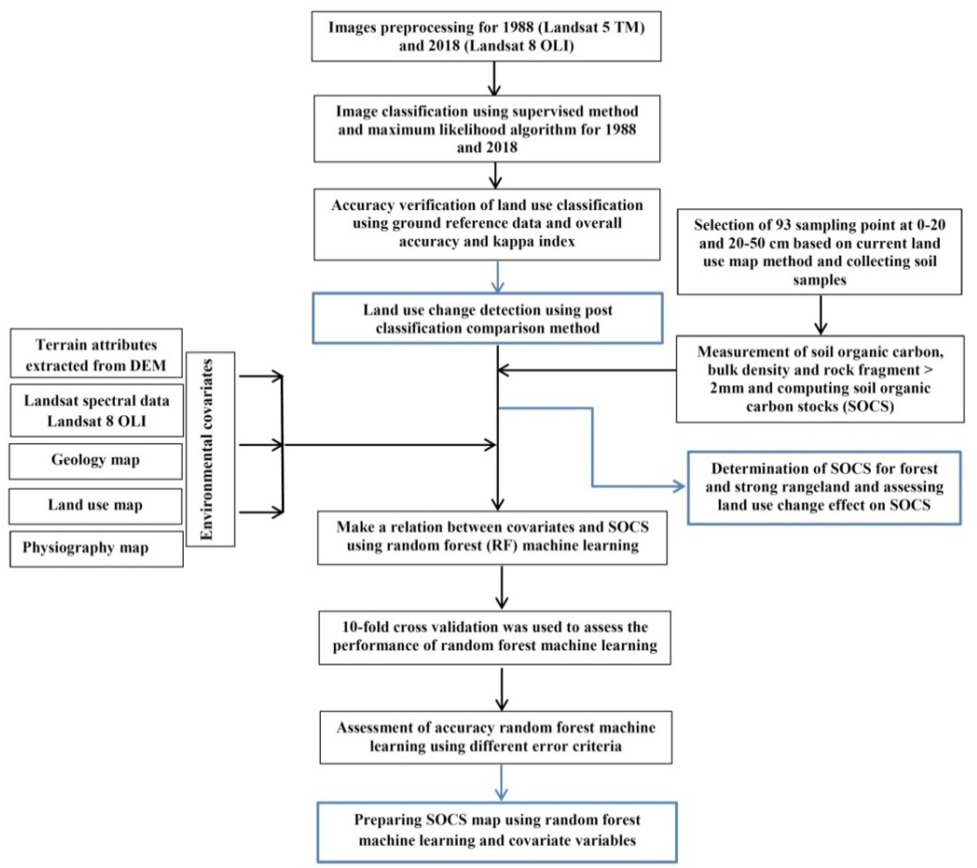
2. Materials and Methods
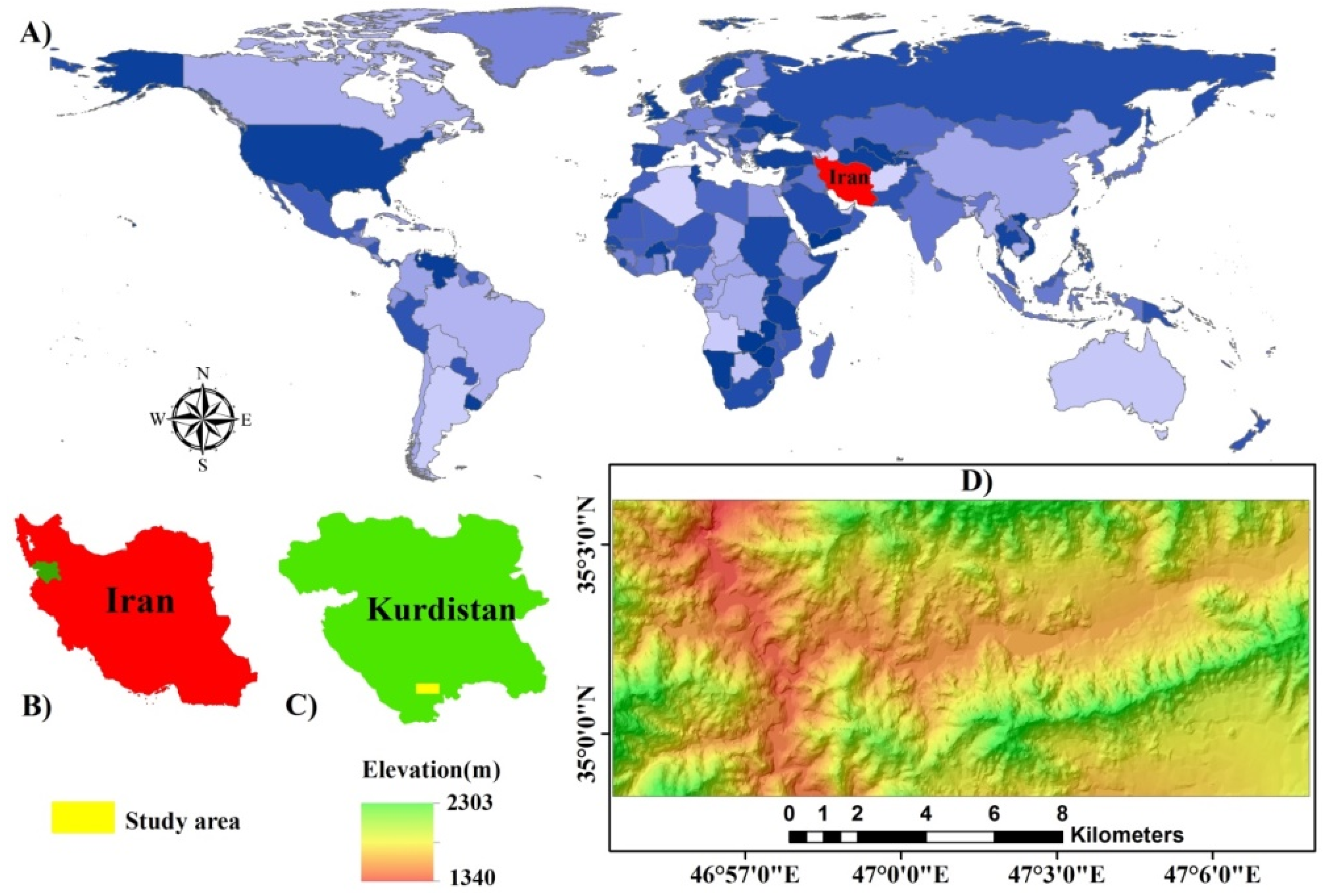
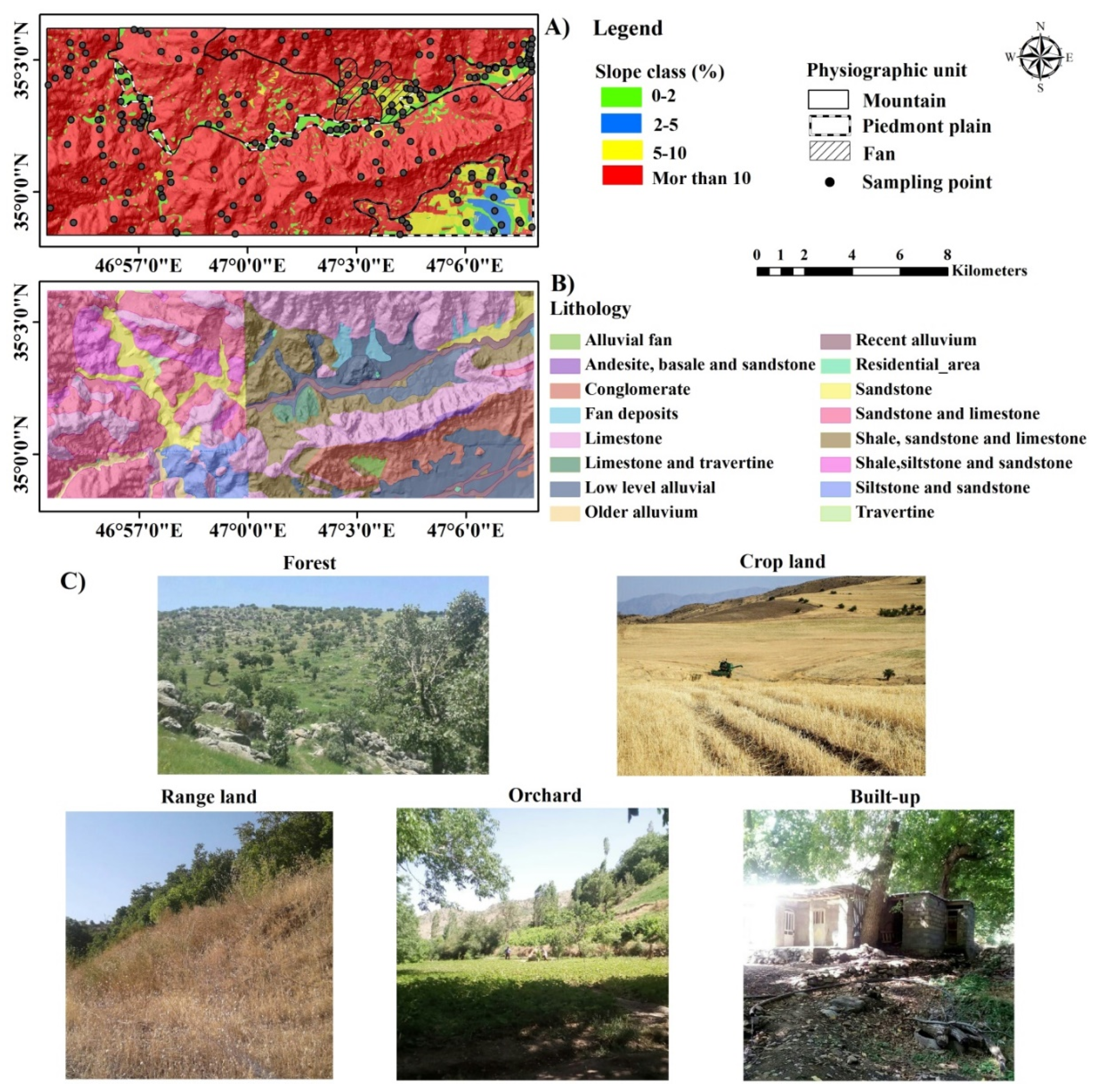
Figure 1 shows a flowchart of the procedures used in this research. In Step 1, remotely sensed data for two time intervals (1988 and 2018) were obtained, pre-processed, and two land use maps were calculated. In Step 2, soil samples were collected and SOCS were calculated. In Step 3, a suite of environmental covariates that were expected to influence SOCS were acquired from various sources (e.g., remote sensing, land-use map, and digital elevation data). These covariates represent the environmental conditions of 2018. In Step 4, a random forest model was used to establish a relationship between covariates and SOCS. Once the random forest model was trained, the model was applied to the suite of environmental covariates to make spatial predictions of soil quality for 2018 in Step 5. To evaluate the historical changes in SOCS, the environmental data that represented 1988 were acquired from satellite imagery and the fitted random forest model was then applied to the historic data in Step 6.

2.1. Study Area

The study area (17,748 ha) is located between 46°54′43.11″ and 47°07′59.1″ E longitude and 34°59′3.41″ and 35°03′33.10″ N latitude, in Kamyaran region, Kurdistan Province, in western Iran (Figure 2). Based on the De Martonne climate classification, the study area has a semi-humid climate with a mean precipitation of 550 mm (Table 1). The altitude of the area ranges from 1340 to 2303 m above sea level. Major agricultural crops include wheat, barley, and orchards (grape, apple, peach, pear, cherry and strawberry). The dominant native vegetation covers are forest (oak and bush-like oaks) and rangeland. These forests have also been called western oak forests and the dominance of oak species are Quercus brantii, Quercus infectoria, Pistacia khenjuk and Pestacia atlantica.

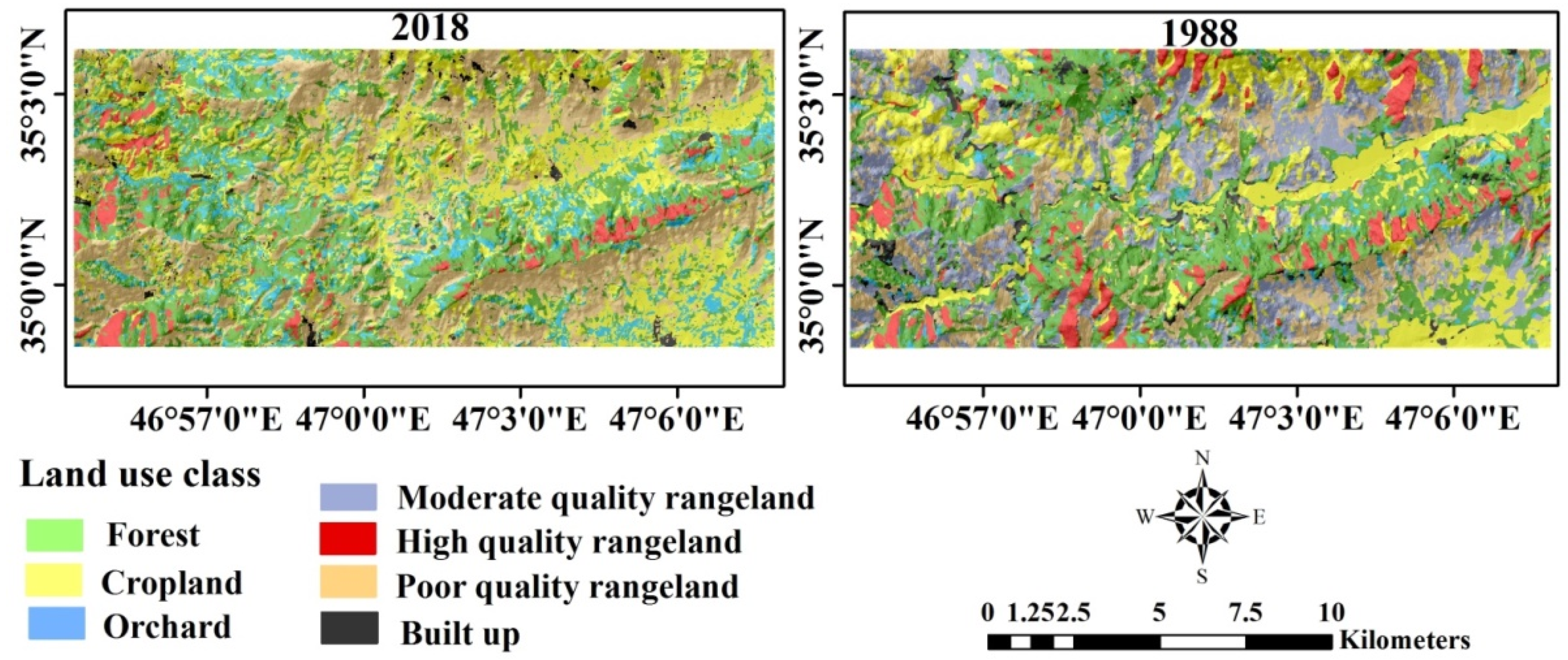
2.2. Land Use Change Detection

Land use changes in the study area were assessed using two multispectral satellite images (1988 and 2018) including Operational Land Imager (OLI)/Landsat 8 and Thematic Mapper (TM)/Landsat 5 from June 23, 1988 and June 27, 2018, respectively [30]. The land use classes included Forest, orchard, cropland, built environment, poor, moderate and high-quality rangeland were identified in the study area based on field visits, Google earth and aerial photo interpretation.
Each satellite image was rectified using pre-processing techniques such as radiometric and geometric corrections. The images were geo-referenced to a topographic map (with a scale of 1:25,000 and Universal Transverse Mercator (UTM) WGS84) using 30 ground control points, and resampling was done through the nearest neighbour method in the R programming environment. For each of the pre-determined land use types, training samples were selected by delimiting polygons around representative sites. A supervised classification method and a maximum likelihood algorithm were applied for accuracy evaluation. Detection of the land use classes was performed in ENVI software (5.3). Maximum likelihood algorithms have been used successfully in supervised classification in the past [11,25,31,32].
Validation of prepared land use maps was done through comparison between the classified images of 1988 and 2018 and ground reference points. Therefore, 100 random ground reference points were selected and gathered based on stratified-random sampling methods, and then, verification of the 1988 and 2018 land use maps was carried out using overall accuracy, kappa index, producer’s accuracy and user’s accuracy [33].
Finally, in the study, the post-classification comparison method was applied to conduct the change detection analyses for 1988–2018 using ENVI (5.3) software as one of the most widely used methods for detection of land use changes [34,35,36,37].

2.3. Soil Organic Carbon Stocks (SOCS)

To characterize the impact of land use on soil organic carbon stocks, 93 sampling sites were selected based on a stratified method using current land use classes including forest, cropland, orchard, high- and poor-quality rangelands and slope classes including 0–2%, 2–5%, 5–10%, and >10% and a total of 186 disturbed and undisturbed soil samples were collected at two depth increments from the surface (0–20 cm) and subsurface (20–50 cm) in 2018 (Figure 3). The soil sampling sites were selected from similar slopes and aspects (Figure 3).
The soil samples were air-dried and passed through 2-mm sieves before any analyses in the laboratory. Soil organic carbon was measured using the Walkley-Black method [38], soil bulk density measurement was conducted by the core method based on the volume of undisturbed core samples and the dry mass after oven-drying [39] and rock fragments > 2 mm were determined using the volumetric method. SOCS were calculated using the following equation (Equation (1)) [11,40]:
SOCS = SOC × BD × d × (1 – RockF/100)
where, SOCS is the SOC stock (Mg ha−1), SOC is the SOC value (g kg−1), BD is bulk density (Mg m−3), d is soil depth thickness (m), and RockF is the volume-based (%) of rock fragments > 2 mm.

2.4. Digital Mapping of SOCS

2.4.1. Environmental Covariates

The set of 30 covariates used for this study were selected due to their relationship to SOCS [25,41,42,43,44,45,46,47]. The majority of the covariates were derived from remote sensing data (i.e., Landsat imagery) as well as from a digital elevation model (DEM). The multi spectral bands of Landsat 8 OLI (operational land imager) and Landsat 5 TM (Thematic Mapper) acquired on June 27, 2018 and 1988, respectively, and the spectral indices from the satellite image were determined including the soil adjusted vegetation index (SAVI) [48], brightness index (BI) [49], normalized difference vegetation index (NDVI) [50], and the clay index (CI) [51], (Table 2). Derived terrain parameters were calculated using a DEM (10 × 10 m grid cell resolution) [52] using SAGA GIS software (System for Automated Geoscientific Analysis) [53] (Table 2). A map of physiography, parent material, land use, temperature and precipitation were also used as environmental covariates. The Mountain, fan and piedmont plain are the major physiographic units and limestone, conglomerate, shale, travertine, alluvium and sandstone are the dominant geological units in this area (Figure 2 and Table 2). All environmental covariates are co-registered to the same raster grid with a size of 30 × 30 m.

2.4.2. Random Forest

In the current research, random forests have been used to make links between SOCS and covariates for understanding the spatial and temporal variability of SOCS [54,55,56,57]. Random forests are one of the most commonly applied machine learning algorithms in DSM due to the good accuracy level, ease of use, and their ability to identify the most important covariates [11,58,59,60,61]. Random forests are ensemble and nonparametric techniques based on the prediction of multiple randomized regression trees. The results of all individual trees are aggregated together to create a singular prediction, whereby randomness is incorporated through a bootstrap sample of the training data and variable selection based on a random subset of the variables at each node [62]. Notably, a random forest is easily adjustable using two tuning hyperparameters: the number of trees (Ntree) and the number of input covariates in each random subset (Mtry). We analyzed the interaction effect of different random subsets (from 2 to 30) and different tree sizes (from 50 to 5000 by increments of 50).
The random forests were assessed through ten-fold cross-validation with 10 replications. Furthermore, three accuracy criteria namely, the root mean square error (RMSE), coefficient of determination (R2) and mean absolute error (MAE), were used to quantify the accuracy of the random forests.

2.5. Reconstructing of SOCS in 1988

We used the trained random forest in 2018 on the covariates sets in 1988 to reconstruct the SOCS maps because we did not have enough soil data (only 10 samples) for training random forest and mapping SOCS in 1988. Importantly, we used 10 legacy data to assess and evaluate the reconstructed SOCS maps in 1988. Furthermore, in the study, only land use maps have changed significantly during the 30-year study. Therefore, to highlight the impact of land use change on SOCS from 1988 to 2018, the SOCS were compared between the two maps.

3. Results and Discussion

3.1. Accuracy Assessment of Land Use Classification

The overall accuracy and the kappa index for the supervised and maximum likelihood classification algorithms for the classification of land use types in 1988 and 2018 are shown in Table 3. The user’s accuracy and producer’s accuracy of individual land uses in 1988 ranged between 84.61% and 100% and 61.53% and 100%. For 2018, the user’s and producer’s accuracy of individual land uses ranged between 64.28% and 100% and 76.92% and 90%, respectively. The overall accuracy for 1988 and 2018 were 88% and 83% with kappa index values of 85 and 78, respectively. The minimum level of land use classification accuracy using remote sensing data is 85% [25,63]. Therefore, our land use classification has an acceptable level of accuracy and other researchers have reported similar results [1,25,64,65].

3.2. Land Use Change Trends

The land use maps developed for 1988 and 2018 using remote sensing methods are shown in Figure 4. The majority of forest and rangeland land use classes are located in the mountain physiographic unit having steep to very steep slopes. However, cropland and orchard land use classes are distributed throughout the study area from the piedmont plain to the mountain physiographic units starting from the low to steep slopes. A clear increase in the orchard, poor-quality rangeland and cropland classes was observed while a clear decrease was observed in the forest, high- and moderate-quality rangeland area during the 30-year study. The area of forest, high- and moderate-quality rangeland changed by approximately 1052.14 ha with a rate of change of −22.27%, 430.44 ha, −29.31%, and 3595.77 ha and −100%, respectively (Table 4). In contrast, the area of poor-quality rangeland, cropland and orchards increased by approximately 1897.92 ha with a rate of increase of 10.73%, 1640.05 ha, 9.29%, and 1748.32 ha and 66.19%, respectively (Table 4). The most dominant changes were the conversion of forest to cropland, moderate-quality rangeland to cropland, cropland to poor-quality rangeland, moderate-quality rangeland to poor-quality rangeland, forest to poor-quality rangeland, forest to orchard, and with converted areas of 8.96%, 6.26%, 6.10, 5.77%, 5.63% and 4.44%, respectively. The spatial trend of cropland and orchard expansion in the forest and rangeland areas from 1988 to 2018 is clearly demonstrated in Figure 4. The area of natural vegetation (forest, high-quality rangeland and moderate-quality rangeland) cover decreased by approximately 5286.29 ha with a decrease of −29.78% over the 30-year study. The natural vegetation has mostly been consumed by cropland and orchard growth, which can be considered as the most important areas of natural vegetation removal in the Kurdistan province. Cropland and orchard expansion, overgrazing in the high and moderate-quality rangeland areas, increasing land prices, lack of vegetation protection policies, and lack of proper supervision and management by government are other factors which have led to the degradation of forests and high-quality rangelands and the expansion of poor-quality rangelands.
These results are similar to the results of Haque and Basak [66], Huang et al. [22], Jombo et al. [23], Sibanda et al. [67], Yin et al. [26], and Zembe et al. [68] who demonstrated spatial-temporal changes in natural vegetation due to unsustainable farming practices, overgrazing and deforestation.
In the study area, a clear decrease also was observed in the built-up area. The built-up area changed by approximately 207.94 ha with a decrease of −34.46% (Table 4) and the most dominant change was the conversion of the built-up area to cropland and poor range lands. The change is mostly affected by the low income of the villagers and migration of villagers towards cities due to lack of government support.

3.3. Summary Statistics of SOC and SOCS

Table 5 shows the descriptive statistics of SOC, SOCS, bulk density and rock fragment in the study area. The average SOC in the surface soil (0–20 cm) and subsurface soil (20–50 cm) are 0.88% and 0.46%, respectively and it ranges from 0.07% to 2.96% in the surface soil and from 0.46% to 2.03% in the subsurface soil. These values indicate that the SOC has low to medium levels. The average SOCS in the surface soil and subsurface soil are 1.67 Mg C ha−1 and 1.28 Mg C ha−1, respectively, and it ranges from 0.7 Mg C ha−1 to 8.18 Mg C ha−1 in the surface soil and from 0.4% to 7.59% in the subsurface soil. The lowest SOC and SOCS were observed for the poor-quality rangeland and cropland, while the highest SOC and SOCS were observed for the high-quality rangeland and forestland. SOC and SOCS decreased with depth and they showed a log-normal distribution. The coefficient of variation (CV) value of SOC and SOCS in the surface soil and subsurface soil were more than 35% indicating a high variability across the study area [69]. Wilding [69] classified values based on the coefficient of variation (CV) into 3 levels with Low (CV < 35%), moderate (15% < CV < 35%) and high variability (CV > 35%). Based on CV analysis, the results indicate that SOCS have a semi-homogeneous spatial variability that could be related to the differences in land use classes, parent material and topography in the study area.

3.4. Link between SOCS and Land Use
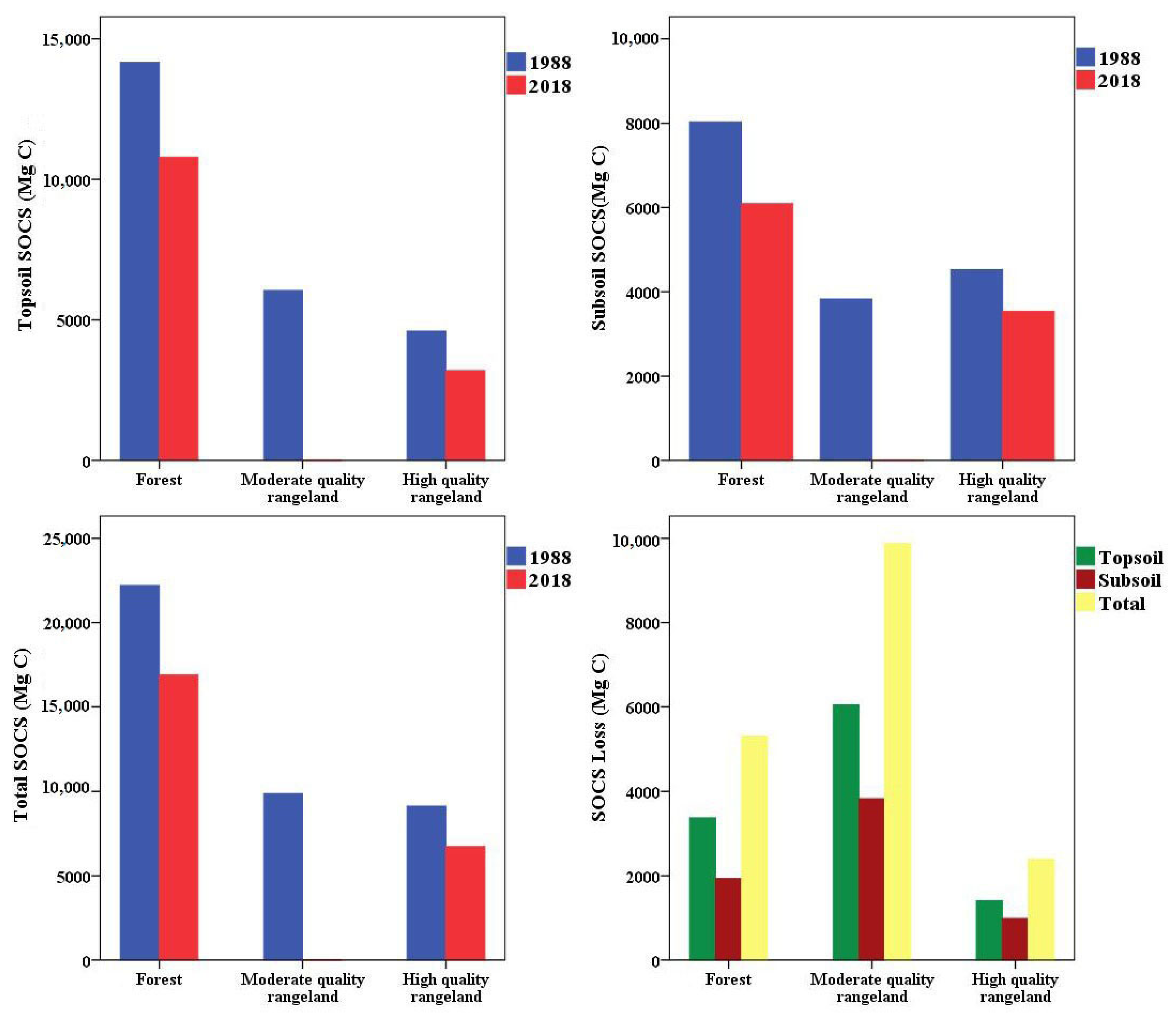
Table 6 shows the mean values of SOCS in the surface soil (0–20 cm), subsurface soil (20–50 cm) and both depths together (0–50 cm) for each land use class in the study area. High-quality rangeland, forest, orchard, cropland, and poor-quality rangeland have 2.94, 3.08, 1.79, 1.49 and 1.17 Mg C ha−1 in the surface soil, 3.41, 1.66, 0.90, 1.39 and 0.90 Mg C ha−1 in the subsurface soil, and 6.49, 4.6, 2.69, 2.88 and 2.07 Mg C ha−1 in total, respectively.
An analysis of variance test was used to compare the mean values of SOCS with respect to land use (Table 6). Based on all soil samples, the mean values of SOCS for the high-quality rangeland and forest in the surface soil (3.08 and 2.94 Mg C ha−1, respectively), subsurface soil (3.41 Mg C ha−1) and total (6.49 and 4.6 Mg C ha−1, respectively) were significantly higher compared to other land use classes.
Based on the slope class 0–2%, the mean values of SOCS for the high-quality rangeland in the surface soil (4.48 Mg C ha−1), subsurface soil (4.12 Mg C ha−1), and total (8.60 Mg C ha−1) were significantly higher than cropland and orchards. Based on the 2–5% slope class, the mean values of SOCS for high-quality rangeland in the surface soil (2.88 Mg C ha−1), subsurface soil (3.61 Mg C ha−1), and total (6.49 Mg C ha−1) were significantly higher compared to other land use classes. Based on the 5–10% slope class, the mean values of SOCS for the high-quality rangeland in the surface soil (3.02 Mg C ha−1), subsurface soil (2.70 Mg C ha−1), and total (5.72 Mg C ha−1) were higher than the other land use classes although not significantly higher. Based on the >10% slope class, the mean values of SOCS for the forest and high-quality rangeland in the surface soil (2.94 and 2.83 Mg C ha−1, respectively), subsurface soil (1.66 and 2.63 Mg C ha−1, respectively), and total (4.6 and 6.49 Mg C ha−1, respectively) were significantly higher in comparison with the other land use classes (Table 6). This result is similar to those of previous studies [40], which indicated that deforestation and cultivation caused 48.2% decrease in SOC of surface soils for a sub humid region in northern Iran. Their results also showed that forestland had significantly higher SOC contents for all slope gradients (< 5%, 5–15%, 15–30% and >30%) [40]. Lizaga also et al. [10] and Wang S. et al. [70] also assessed the effect of natural vegetation transformation (forest and grassland) to cropland on SOC in Spain and China, respectively. They showed that afforested and natural forest areas had the highest SOC and total nitrogen contents, and agricultural land had the lowest SOC and total nitrogen contents due to loss by erosion and cultivation. Removal of natural vegetation, due to anthropogenic activities, is a major global cause of land use change [71,72,73] which causes land degradation [74,75].
Removal of natural vegetation has negative impacts on soil quality [71,76,77]. SOCS is one of the main indices for assessing the effect of land use change on soil quality [11,78,79] and is very sensitive to land use type and its management [16,80,81]. It also diverges with variations of land use and cover.
These findings showed that land use type is one of the most important parameters responsible for SOCS levels which decrease with land use change from natural vegetation to cropland and orchard in the study area. Besides land use change, conventional agriculture, over grazing and lack of vegetation protection policies and proper management have led to accelerated decreases in SOCS in the study area.

3.5. SOCS Loss

Based on the changed area of forest, high- and moderate-quality rangeland and their SOCS content, the loss of carbon was calculated for the forest and high-quality rangeland (Figure 5 and Table 4). Approximately 1052.14 ha of the forests have been converted to other land uses and this conversion has caused a decrease of approximately 3376.69 Mg C from the surface soil (0–20 cm), 1935.48 Mg C from the subsurface soil (20–60 cm) and 5312.17 Mg C from the total (0–50 cm) in SOCS compared to the forest that was cleared (Figure 5). About 430.44 ha and 3595.77 ha of the high- and moderate-quality rangelands, respectively, have been converted to other land uses and this conversion has caused a decrease in SOCS of between 1404.95 Mg C and 6047.60 Mg C from the surface soil (0–20 cm), 987.10 Mg C and 3828.52 Mg C from the surface soil (20–60 cm), and 2392.06 Mg C and 9876.12 from both depths combined (0–50 cm) compared to the high-quality rangeland that was cleared (Figure 5). In general, removal of natural vegetation cover (forest and moderate and high-quality rangelands) led to the loss of 10,829.25 Mg C in the surface soil, 6751.11 Mg C in the surface soil, and 17,580.36 Mg C in the total, respectively.
Nabiollahi et al. [11] also assessed SOCS under land-use changes in Marivan region, Iran and they indicated that converting forestland and wetland to cropland caused a loss of SOCS from surface soil (22,860 and 4193 Mg C, respectively) and subsurface soil (15,685 and 2680 Mg C, respectively); those results were similar to our results.
Depletion of SOCS and transformation of natural vegetation are some of the most important reasons for greenhouse gases increasing and climate changing in the last 100 years [82,83,84]. Soil is one of the most important ecosystem components and third most important carbon stores [80,85]. In addition, to balancing climate change soil carbon sequestration is suggested for decreasing CO2 and for reserving and increasing soil carbon stocks [86,87,88]. Due to the effects of SOC on soil physical, chemical and biological properties such as water holding capacity and availability, aggregate stability, soil erodibility and fertility, nutrient cycling and plant growth, it has an important role in sustainable land management.

3.6. Digital Mapping of SOCS

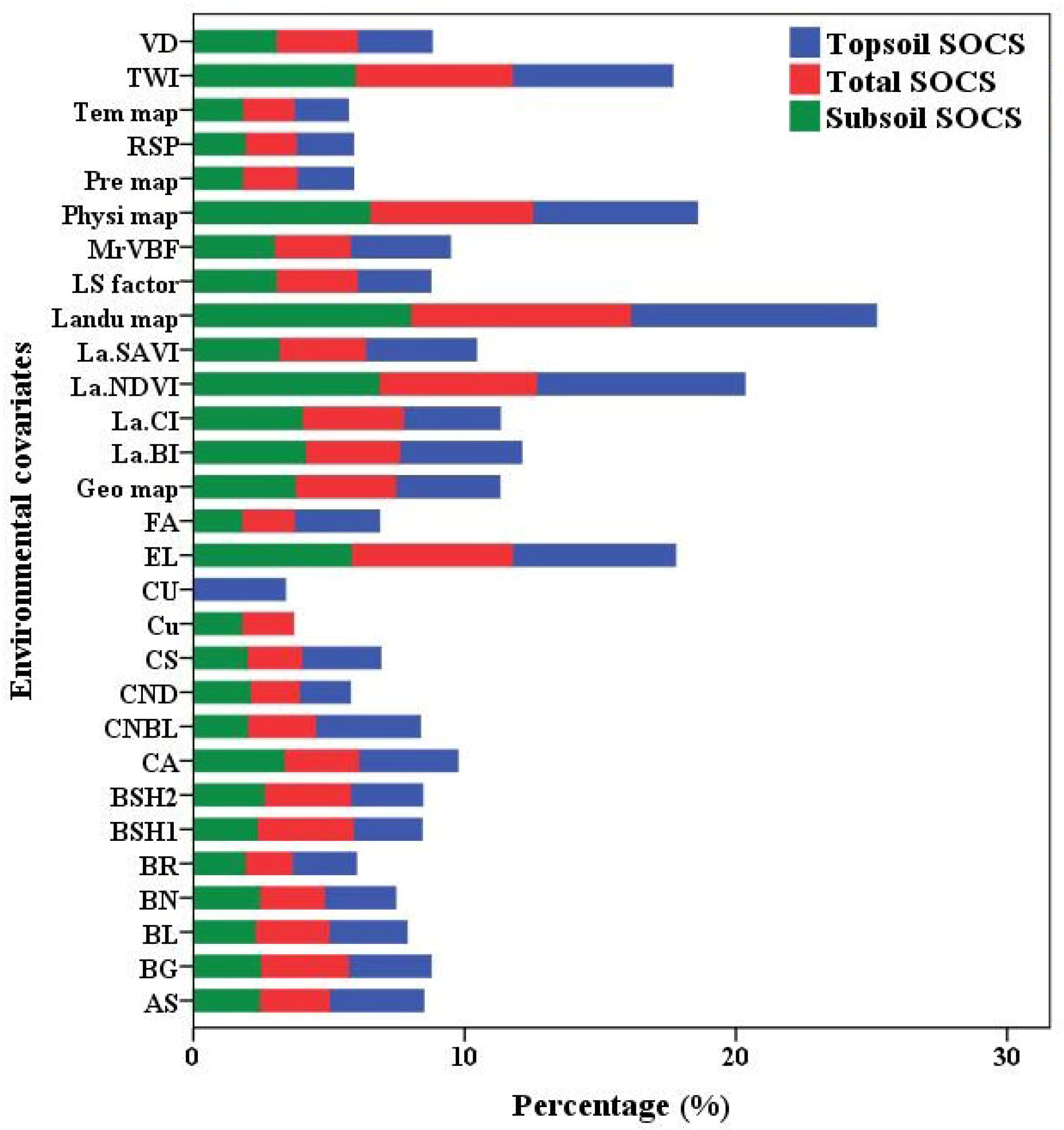
3.6.1. Covariate Importance

Figure 6 shows the significance of each applied environmental covariates in predicting SOCS. In terms of predicting surface, subsurface and total SOCS for the 2018 land use map (9.08, 8.00 and 8.10), NDVI (7.68, 6.48 and 5.80), physiographic map (6.08, 6.50, and 6.00), topographic wetness index (5.91, 5.95 and 5.8) and elevation (6.01, 5.8, and 5.96) were the six most important environmental variables. These findings indicate that data extracted from remote sensing imagery, land use and terrain attributes are powerful covariates for predicting surface SOCS in the study area. It is demonstrated that land cover, remotely sensed imagery and DEM derivatives are important factors for determining surface SOC [44] and they have been widely applied for prediction of SOC in previous studies for Iran [11,89,90] and the world [46,91,92,93]. Guo et al. [94] and Zhou et al. [18] mapped SOC using different machine learning algorithms and environmental variables in China and their results showed that SOC has strong associations with spectral bands and vegetation indices such as NDVI, EVI and RVI. Ellili et al. [95] also mapped SOCS between 2009 and 2016 in France using different models and covariate variables and showed that slope, wetness index, elevation, profile curvature, tangential curvature, geology map and crop rotation were the most important variables for predicting SOCS. The validation was obtained based on 10 legacy soil sample data.

3.6.2. Random Forests

The ability of the random forest algorithm to predict surface, subsurface and total SOCS, in the Kamyaran region were tested using 10-fold cross-validation with 10 replications. The RMSEs, R2 values, and MAEs, are presented in Figure 7. Across all accuracy metrics (RMSE, R2 and MAE), the random forest algorithm had acceptable accuracy for prediction of surface SOCS (0.70, 0.66 and 0.72, for 2018 and 0.96, 0.46 and 1.01, for 1988, respectively), subsurface SOCS (0.69, 0.67 and 0.69, for 2018 and 0.94, 0.48 and 1.01, for 1988, respectively) and total SOCS (0.74, 0.63 and 0.51, for 2018 and 0.99, 0.47 and 1.04, for 1988, respectively). The success in using random forest machine learning was also reported by Akpa et al. [86], Lamichhane et al. [44], Wang B. et al. [59] and Zhou et al. [18] for predicting SOC; and therefore, it can be suggested that this machine learning algorithm could show promise in subsequent DSM studies.

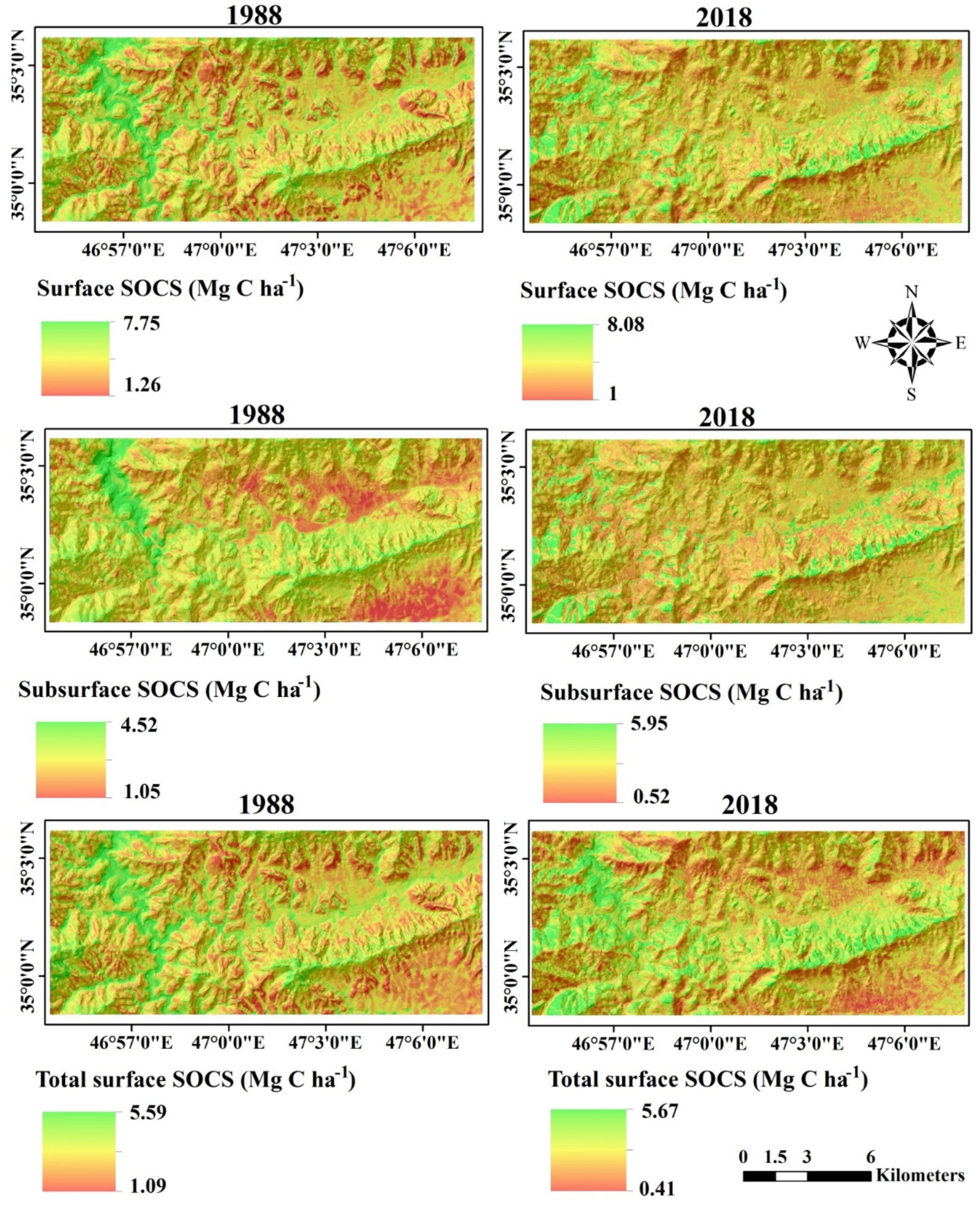
3.6.3. Spatial Distribution of SOCS

Figure 7 shows the DSM of SOCS at three depths for 1988 and 2018 prepared through the RF algorithm. The maps show that the majority of the areas with high levels of predicted SOCS are concentrated in the center, north, east, northwestern, and southwestern mountainous areas of the study area mostly covered by forest and high-quality rangeland. In contrast, lower SOCS are mainly concentrated in poor-quality rangeland, cropland, and orchards in the south, southeastern, and central part of the study area.
This result reflected the effect of vegetation type on the variability of SOCS. The important role of vegetation type to predict SOCS has been demonstrated by other studies [18,44,46]. Moreover, differences in terrain attributes affect SOCS using its relationship with vegetation cover. The mountain areas of this study area had higher SOC content and were mostly covered by high-quality rangeland and forest. Conversely, lower lands had lower SOC contents and were mostly covered by farmland and orchard. These results are similar to the results of Schulze and Schütte [19] and Zhou et al. [18] who indicated that cropland has lower SOC contents compared to the natural vegetation due to the loss of SOCS by clearing natural land resources. The SOCS map is essential for helping to decrease climate change and greenhouses gas emissions, land use change and degradation and increasing environmental monitoring, improving farm operations and increasing crop production. As was shown in the study, anthropogenic activities such as cultivation and overgrazing in general cause a reduction in SOCS. Therefore, it is suggested that conservation agricultural operations (conventional tillage is a common tillage operation and the depth of the tillage layer is 30 cm) are adopted (e.g., the construction of contour banks, minimum tillage or no tillage), that over grazing and conversion of natural vegetation to other land uses (e.g., cropland, orchard and built-up) is discouraged to prevent land degradation, SOCS depletion, and greenhouse gases increasing in the study area. Other studies have shown that policies of natural vegetation degradation abandonment and natural revegetation can help to control natural vegetation removal. Lizaga et al. [10] demonstrated that after a land abandonment policy of natural transformation was applied, cropped areas decreased by 16.5%, while in contrast, afforestation and natural revegetation areas were increased to 83.5% of the study area. Akinyemi et al. [21] also indicated that the government’s policy led to an increase in the national forest of 30% in Rwanda. The majority of natural vegetation conversion in the study area was done by villagers due to need for food so funding and social government support is essential for sustainable land management.

4. Conclusions

Land use change and SOCS maps that identify areas of high risk of degradation can be used for sustainable land management and decreasing the effects of these changes on the environment. This study assessed the spatial and temporal distribution of land use transformation and SOCS depletion in the Kamyaran region of the Kurdistan province, Iran. The integration of supervised classification, post-classification, and satellite images from the beginning and end of the study period (1988–2018) were applied to develop land use maps for 1988 and 2018. Seven land use types have been identified, which are forest, cropland, built-up, orchard, high, moderate, and poor-quality rangeland. The crop land and poor-quality rangeland areas were the most abundant land use categories in the study area. Over the 30-year study, a clear increase was observed in orchards, poor-quality rangeland and cropland, and a clear decrease was observed in the forest, high-quality rangeland, moderate-quality rangeland, and built-up area; this is mostly due to the increasing need for food and anthropogenic activities such as cultivation and over grazing and lack of government decision-making policies.
The clearing of natural vegetation cover (forest, high- and moderate-quality rangeland) causes decreases in SOCS. Therefore, to reduce the challenge of natural vegetation conversion to other uses, SOCS depletion and greenhouse gas increase, applying suitable strategies e.g., conservation agriculture operations, the discouraging over grazing and natural vegetation conversion to other land uses, and increasing villagers’ awareness of the value of natural vegetation through the government are required. It is also recommended that additional research to assess the scenarios of natural vegetation degradation through interpretation of a continuous time series of remote sensing images is undertaken for swift decision making.

Author Contributions

Conceptualization—K.N., S.S. and S.Z.; methodology—K.N., S.S., S.Z. and R.T.-M.; software—K.N., S.S., S.Z. and R.T.-M.; analysis—K.N., S.Z., R.T.-M., R.K. and T.S.; investigation—K.N., S.S. and S.Z.; data curation—K.N., S.S. and S.Z.; writing—original draft preparation—K.N., R.T.-M., R.K. and T.S; visualization—K.N., S.S. and S.Z. All authors have read and agreed to the published version of the manuscript.

Funding

The University of Kurdistan funded this research and Ruhollah Taghizadeh-Mehrjardi was funded by the Alexander von Humboldt Foundation grant number Ref 3.4-1164573-IRN-GFHERMES-P.

Institutional Review Board Statement

Not applicable.

Informed Consent Statement

Not applicable.

Data Availability Statement

The data presented in this study are available on request from the corresponding author. The data are not publicly available due to privacy restrictions.

Acknowledgments

This study was part of a master project entitled “Change detection of land use change and assessing its effect on soil organic carbon stocks”. Thomas Scholten thanks the German Research Foundation (DFG) for supporting this research through the Collaborative Research Center (SFB 1070) ‘Resource Cultures’ (subprojects Z, S and B02). He is also supported by the DFG Cluster of Excellence “Machine Learning—New Perspectives for Science”, EXC 2064/1, project number 390727645.

Conflicts of Interest

The authors declare no conflict of interest.

References

  1. Crowson, M.; Hagensieker, R.; Waske, B. Mapping land cover change in northern Brazil with limited training data. Int. J. Appl. Earth Obs. Geoinf. 2019, 78, 202–214. [Google Scholar] [CrossRef]
  2. Du, P.; Wang, X.; Chen, D.; Liu, S.; Lin, G.; Meng, Y. An improved change detection approach using tri-temporal log-ic-verified change vector analysis. ISPRS J. Photogramm. 2020, 161, 278–293. [Google Scholar] [CrossRef]
  3. Xi, W.; Du, S.; Wang, Y.-C.; Zhang, X. A spatiotemporal cube model for analyzing satellite image time series: Application to land-cover mapping and change detection. Remote Sens. Environ. 2019, 231, 111212. [Google Scholar] [CrossRef]
  4. Green, J.K.; Seneviratne, S.I.; Berg, A.M.; Findell, K.L.; Hagemann, S.; Lawrence, D.M.; Gentine, P. Large influence of soil moisture on long-term terrestrial carbon uptake. Nat. Cell Biol. 2019, 565, 476–479. [Google Scholar] [CrossRef]
  5. Thomas, A.; Cosby, B.; Henrys, P.; Emmett, B. Patterns and trends of topsoil carbon in the UK: Complex interactions of land use change, climate and pollution. Sci. Total Environ. 2020, 729, 138330. [Google Scholar] [CrossRef]
  6. Wiesmeier, M.; Urbanski, L.; Hobley, E. Soil organic carbon storage as a key function of soils—A review of drivers and in-dicators at various scales. Geoderma 2019, 333, 149–162. [Google Scholar] [CrossRef]
  7. Batjes, N.H. Total carbon and nitrogen in the soils of the world. Eur. J. Soil Sci. 1996, 47, 151–163. [Google Scholar] [CrossRef]
  8. Lal, R. Soil Carbon Sequestration Impacts on Global Climate Change and Food Security. Sustainability 2004, 304, 1623–1627. [Google Scholar] [CrossRef] [Green Version]
  9. Smith, P.; Chapman, S.J.; Scott, W.A.; Black, H.I.J.; Wattenbach, M.; Milne, R.; Campbell, C.D.; Lilly, A.; Ostle, N.; Levy, P.E.; et al. Climate change cannot be entirely responsible for soil carbon loss observed in England and Wales, 1978–2003. Glob. Chang. Biol. 2007, 13, 2605–2609. [Google Scholar] [CrossRef]
  10. Lizaga, I.; Quijano, L.; Gaspar, L.; Ramos, M.C.; Navas, A. Linking land use changes to variation in soil properties in a Mediterranean mountain agroecosystem. Catena 2019, 172, 516–527. [Google Scholar] [CrossRef]
  11. Nabiollahi, K.; Eskandari, S.; Taghizadeh-Mehrjardi, R.; Kerry, R.; Triantafilis, J. Assessing soil organic carbon stocks under land-use change scenarios using random forest models. Carbon Manag. 2019, 10, 63–77. [Google Scholar] [CrossRef]
  12. Xu, E.; Zhang, H.; Xu, Y. Exploring land reclamation history: Soil organic carbon sequestration due to dramatic oasis ag-riculture expansion in arid region of Northwest China. Ecol. Indic. 2020, 108, 105746. [Google Scholar] [CrossRef]
  13. Cannell, M. Forests as carbon sinks mitigating the greenhouse effect. Commonw. For. Rev. 1996, 75, 92–99. [Google Scholar]
  14. Gartzia-Bengoetxea, N.; Gonzalez-Arias, A.; Merino, A.; Martinez de Arano, I. Soil organic matter in soil physical fractions in adjacent semi-natural and cultivated stands in temperate Atlantic forests. Soil Biol. Biochem. 2009, 41, 1674–1683. [Google Scholar] [CrossRef]
  15. Liu, X.; Li, L.; Qi, Z.; Han, J.; Zhu, Y. Land-use impacts on profile distribution of labile and recalcitrant carbon in the Ili River Valley, northwest China. Sci. Total Environ. 2017, 586, 1038–1045. [Google Scholar] [CrossRef]
  16. Miller, G.; Rees, R.; Griffiths, B.; Ball, B.; Cloy, J. The sensitivity of soil organic carbon pools to land management varies depending on former tillage practices. Soil Tillage Res. 2019, 194, 104299. [Google Scholar] [CrossRef]
  17. Zhang, Z.; Wang, J.J.; Lyu, X.; Jiang, M.; Bhadha, J.; Wright, A. Impacts of land use change on soil organic matter chemistry in the Everglades, Florida—A characterization with pyrolysis-gas chromatography–mass spectrometry. Geoderma 2019, 338, 393–400. [Google Scholar] [CrossRef]
  18. Zhou, T.; Geng, Y.; Chen, J.; Pan, J.; Haase, D.; Lausch, A. High-resolution digital mapping of soil organic carbon and soil total nitrogen using DEM derivatives, Sentinel-1 and Sentinel-2 data based on machine learning algorithms. Sci. Total Environ. 2020, 729, 138244. [Google Scholar] [CrossRef]
  19. Schulze, R.E.; Schütte, S. Mapping soil organic carbon at a terrain unit resolution across South Africa. Geoderma 2020, 373, 114447. [Google Scholar] [CrossRef]
  20. Pal, S.; Ziaul, S. Detection of land use and land cover change and land surface temperature in English Bazar urban centre. Egypt. J. Remote Sens. Space Sci. 2017, 20, 125–145. [Google Scholar] [CrossRef] [Green Version]
  21. Akinyemi, F.O. Land change in the central Albertine rift: Insights from analysis and mapping of land use-land cover change in north-western Rwanda. Appl. Geogr. 2017, 87, 127–138. [Google Scholar] [CrossRef]
  22. Huang, H.B.; Chen, Y.L.; Clinton, N.; Wang, J.; Wang, X.Y.; Liu, C.X.; Gong, P.; Yang, J.; Bai, Y.Q.; Zheng, Y.M.; et al. Mapping major land cover dynamics in Beijing using all Landsat images in Google Earth Engine. Remote Sens. Environ. 2017, 202, 166–176. [Google Scholar] [CrossRef]
  23. Jombo, S.; Adam, E.; Odindi, J. Quantification of landscape transformation due to the Fast Track Land Reform Programme (FTLRP) in Zimbabwe using remotely sensed data. Land Use Policy 2017, 68, 287–294. [Google Scholar] [CrossRef]
  24. Giuliani, G.; Dao, H.; de Bono, A.; Chatenoux, B.; Allenbach, K.; de Laborie, P.; Rodila, D.; Alexandris, N.; Peduzzi, P. Live Monitoring of Earth Surface (LiMES): A framework for monitoring environmental changes from Earth Observations. Remote Sens. Environ. 2017, 202, 222–233. [Google Scholar] [CrossRef]
  25. Alijani, Z.; Hosseinali, F.; Biswas, A. Spatio-temporal evolution of agricultural land use change drivers: A case study from Chalous region, Iran. J. Environ. Manag. 2020, 262, 110326. [Google Scholar] [CrossRef]
  26. Yin, H.; Pflugmacher, D.; Li, A.; Li, Z.; Hostert, P. Land use and land cover change in Inner Mongolia—Understanding the effects of China’s re-vegetation programs. Remote Sens. Environ. 2018, 204, 918–930. [Google Scholar] [CrossRef]
  27. Kumar, S.; Shwetank; Jain, K. A Multi-Temporal Landsat Data Analysis for Land-use/Land-cover Change in Haridwar Region using Remote Sensing Techniques. Procedia Comput. Sci. 2020, 171, 1184–1193. [Google Scholar] [CrossRef]
  28. Salem, M.; Tsurusaki, N.; Divigalpitiya, P. Remote sensing-based detection of agricultural land losses around Greater Cairo since the Egyptian revolution of 2011. Land Use Policy 2020, 97, 104744. [Google Scholar] [CrossRef]
  29. Mei, A.; Manzo, C.; Fontinovo, G.; Bassani, C.; Allegrini, A.; Petracchini, F. Assessment of land cover changes in Lampedusa Island (Italy) using Landsat TM and OLI data. J. Afr. Earth Sci. 2016, 122, 15–24. [Google Scholar] [CrossRef]
  30. USGS. Product Guide: Provisional Landsat 8 Surface Reflectance Product Guide; USGS: Reston, VA, USA, 2018.
  31. Mosammam, H.M.; Nia, J.T.; Khani, H.; Teymouri, A.; Kazemi, M. Monitoring land use change and measuring urban sprawl based on its spatial forms: The case of Qom city. Egypt. J. Remote Sens. Space Sci. 2017, 20, 103–116. [Google Scholar]
  32. Singh, P.; Kikon, N.; Verma, P. Impact of land use change and urbanization on urban heat island in Lucknow city, Central India. A remote sensing based estimate. Sustain. Cities Soc. 2017, 32, 100–114. [Google Scholar] [CrossRef]
  33. Foody, G.M. Status of land cover classification accuracy assessment. Remote Sens. Environ. 2002, 80, 185–201. [Google Scholar] [CrossRef]
  34. Abd-EL-kawy, O.R.; Ismail, H.A.; Yehia, H.M. Temporal detection and prediction of agricultural land consumption by urbanization using remote sensing. Egypt. J. Remote Sens. Space Sci. 2019, 22, 237–246. [Google Scholar] [CrossRef]
  35. Mishra, S.; Shrivastava, P.; Dhurvey, P. Maulana Azad National Institute of Technology Bhopal Change Detection Techniques in Remote Sensing: A Review. Int. J. Wirel. Mob. Commun. Ind. Syst. 2017, 4, 1–8. [Google Scholar] [CrossRef]
  36. Raja, R.A.A.; Anand, V.; Kumar, A.S.; Maithani, S.; Kumar, V.A. Wavelet Based Post Classification Change Detection Technique for Urban Growth Monitoring. J. Indian Soc. Remote Sens. 2013, 41, 35–43. [Google Scholar] [CrossRef]
  37. Wu, C.; Du, B.; Cui, X.; Zhang, L. A post-classification change detection method based on iterative slow feature analysis and Bayesian soft fusion. Remote Sens. Environ. 2017, 199, 241–255. [Google Scholar] [CrossRef]
  38. Nelson, D.W.; Sommers, L.E. Total Carbon, Organic Carbon, and Organic Matter. In Methods of Soil Analysis, Part 2-Chemical and Microbiological Properties; Page, A.L., Miller, R.H., Keeney, D.R., Eds.; ASA-SSSA: Madison, WI, USA, 1982; pp. 539–594. [Google Scholar]
  39. Grossman, R.B.; Reinsch, T.G. 2.1 Bulk Density and Linear Extensibility; Wiley: Hoboken, NJ, USA, 2018; pp. 201–228. [Google Scholar]
  40. Ajami, M.; Heidari, A.; Khormali, F.; Gorji, M.; Ayoubi, S. Environmental factors controlling soil organic carbon storage in loess soils of a subhumid region, northern Iran. Geoderma 2016, 281, 1–10. [Google Scholar] [CrossRef]
  41. Adhikari, K.; Hartemink, A.E. Soil organic carbon increases under intensive agriculture in the Central Sands, Wisconsin, USA. Geoderma Reg. 2017, 10, 115–125. [Google Scholar] [CrossRef]
  42. Hamzehpour, N.; Shafizadeh-Moghadam, H.; Valavi, R. Exploring the driving forces and digital mapping of soil organic carbon using remote sensing and soil texture. Catena 2019, 182, 104141. [Google Scholar] [CrossRef]
  43. Keskin, H.; Grunwald, S.; Harris, W.G. Digital mapping of soil carbon fractions with machine learning. Geoderma 2019, 339, 40–58. [Google Scholar] [CrossRef]
  44. Lamichhane, S.; Kumar, L.; Wilson, B. Digital soil mapping algorithms and covariates for soil organic carbon mapping and their implications: A review. Geoderma 2019, 352, 395–413. [Google Scholar] [CrossRef]
  45. Minasny, B.; McBratney, A.B.; Malone, B.P.; Wheeler, I. Digital Mapping of Soil Carbon. Adv. Agron. 2013, 118, 1–47. [Google Scholar] [CrossRef]
  46. Rial, M.; Cortizas, A.M.; Rodríguez-Lado, L. Understanding the spatial distribution of factors controlling topsoil organic carbon content in European soils. Sci. Total Environ. 2017, 609, 1411–1422. [Google Scholar] [CrossRef]
  47. Schillaci, C.; Acutis, M.; Lombardo, L.; Lipani, A.; Fantappie, M.; Marker, M.; Saia, S. Spatio-temporal topsoil organic carbon mapping of a semi-arid Mediterranean region: The role of land use, soil texture, topographic indices and the influence of the remote sensing data to modeling. Sci. Total Environ. 2017, 601, 821–832. [Google Scholar] [CrossRef]
  48. Huete, A. A soil-adjusted vegetation index (SAVI). Remote Sens. Environ. 1988, 25, 295–309. [Google Scholar] [CrossRef]
  49. Metternicht, G.; Zinck, J. Remote sensing of soil salinity: Potentials and constraints. Remote Sens. Environ. 2003, 85, 1–20. [Google Scholar] [CrossRef]
  50. Rouse, J.W.; Hass, R.H.; Schell, J.A.; Deering, D.W. Monitoring vegetation systems in the Great Plains with ERTS. In Technical Presentations Section A Proceedings of the NASA SP-351: Third Earth Resources Technology Satellite-Symposium, Washington, DC, USA, 10–14 December 1973; Freden, S.C., Mercanti, E.P., Becker, M.A., Eds.; NASA Science and Technology Information: Washington, DC, USA, 1974; Volume 1, pp. 309–317. [Google Scholar]
  51. Boettinger, J.; Ramsey, R.; Bodily, J.; Cole, N.; Kienast-Brown, S.; Nield, S.; Saunders, A.; Stum, A. Landsat Spectral Data for Digital Soil Mapping. In Digital Soil Mapping with Limited Data; Metzler, J.B., Ed.; Springer: Berlin/Heidelberg, Germany, 2008; pp. 193–202. [Google Scholar]
  52. National Cartographic Center of Iran, Research Institute of National Cartographic Center, Tehran, Iran. 2014. Available online: http://www.ncc.org.ir/ (accessed on 14 February 2014).
  53. Olaya, V. A Gentle Introduction to SAGA GIS; The SAGA User Group e.V.: Gottingen, Germany, 2004; p. 216. [Google Scholar]
  54. Malone, B.P.; Jha, S.K.; Minasny, B.; McBratney, A.B. Comparing regression-based digital soil mapping and multiple-point geostatistics for the spatial extrapolation of soil data. Geoderma 2016, 262, 243–253. [Google Scholar] [CrossRef]
  55. McBratney, A.; Santos, M.M.; Minasny, B. On digital soil mapping. Geoderma 2003, 117, 3–52. [Google Scholar] [CrossRef]
  56. Minasny, B.; McBratney, A. Digital soil mapping: A brief history and some lessons. Geoderma 2016, 264, 301–311. [Google Scholar] [CrossRef]
  57. Teng, H.; Rossel, R.A.V.; Shi, Z.; Behrens, T. Updating a national soil classification with spectroscopic predictions and digital soil mapping. Catena 2018, 164, 125–134. [Google Scholar] [CrossRef]
  58. Taghizadeh-Mehrjardi, R.; Nabiollahi, K.; Rasoli, L.; Kerry, R.; Scholten, T. Land Suitability Assessment and Agricultural Production Sustainability Using Machine Learning Models. Agronomy 2020, 10, 573. [Google Scholar] [CrossRef]
  59. Wang, B.; Waters, C.; Orgill, S.; Gray, J.; Cowie, A.; Clark, A.; Liu, D.L. High resolution mapping of soil organic carbon stocks using remote sensing variables in the semi-arid rangelands of eastern Australia. Sci. Total Environ. 2018, 630, 367–378. [Google Scholar] [CrossRef]
  60. Zeraatpisheh, M.; Bakhshandeh, E.; Hosseini, M.; Alavi, S.M. Assessing the effects of deforestation and intensive agriculture on the soil quality through digital soil mapping. Geoderma 2020, 363, 114139. [Google Scholar] [CrossRef]
  61. Zhou, T.; Geng, Y.; Chen, J.; Liu, M.; Haase, D.; Lausch, A. Mapping soil organic carbon content using multi-source remote sensing variables in the Heihe River Basin in China. Ecol. Indic. 2020, 114, 106288. [Google Scholar] [CrossRef]
  62. Breiman, L. Random Forests. Mach. Learn. 2001, 45, 12–20. [Google Scholar]
  63. Anderson, J.R.; Hardy, E.E.; Roach, J.T.; Witmer, R.E. A Land Use and Land Cover Classification System for Use with Remote Sensor Data; US Geological Survey: Reston, VA, USA, 1976; Volume 964. [Google Scholar]
  64. Piquer-Rodríguez, M.; Butsic, V.; Gärtner, P.; Macchi, L.; Baumann, M.; Pizarro, G.G.; Volante, J.; Gasparri, I.; Kuemmerle, T. Drivers of agricultural land-use change in the Argentine Pampas and Chaco regions. Appl. Geogr. 2018, 91, 111–122. [Google Scholar] [CrossRef]
  65. Watmough, G.R.; Palm, C.A.; Sullivan, C. An operational framework for object-based land use classification of heteroge-neous rural landscapes. Int. J. Appl. Earth Obs. Geoinf. 2017, 54, 134–144. [Google Scholar] [CrossRef]
  66. Haque, M.I.; Basak, R. Land cover change detection using GIS and remote sensing techniques: A spatio-temporal study on Tanguar Haor, Sunamganj, Bangladesh. Egypt. J. Remote Sens. Space Sci. 2017, 20, 251–263. [Google Scholar] [CrossRef]
  67. Sibanda, M.; Dube, T.; Mubango, T.; Shoko, C. The utility of earth observation technologies in understanding impacts of land reform in the eastern region of Zimbabwe. J. Land Use Sci. 2016, 11, 384–400. [Google Scholar] [CrossRef]
  68. Zembe, N.; Mbokochena, E.; Mudzengere, F.H.; Chikwriri, E. An assessment of the impact of the fast track land reform programme on the environment: The case of eastdale farm in gutu district masvingo. J. Geogr. Reg. Plan. 2014, 7, 160–175. [Google Scholar]
  69. Wilding, L.P. Spatial variability: Its documentation, accommodation and implication to soil surveys. In Proceedings of the Soil Spatial Variability, Las Vegas, NV, USA, 30 November–1 December 1985; pp. 166–194. [Google Scholar]
  70. Wang, S.; Adhikari, K.; Wang, Q.; Jin, X.; Li, H. Role of environmental variables in the spatial distribution of soil carbon (C), nitrogen (N), and C:N ratio from the northeastern coastal agroecosystems in China. Ecol. Indic. 2018, 84, 263–272. [Google Scholar] [CrossRef]
  71. Davari, M.; Gholami, L.; Nabiollahi, K.; Homaee, M.; Jafari, H.J. Deforestation and cultivation of sparse forest impacts on soil quality (case study: West Iran, Baneh). Soil Tillage Res. 2020, 198, 104504. [Google Scholar] [CrossRef]
  72. Tesfaye, M.A.; Bravo, F.; Ruiz-Peinado, R.; Pando, V.; Bravo-Oviedo, A. Impact of changes in land use, species and ele-vation on soil organic carbon and total nitrogen in Ethiopian central highlands. Geoderma 2016, 261, 70–79. [Google Scholar] [CrossRef]
  73. Villarino, S.H.; Studdert, G.A.; Baldassini, P.; Cendoya, M.G.; Ciuffoli, L.; Mastrángelo, M.; Piñeiro, G. Deforestation impacts on soil organic carbon stocks in the Semiarid Chaco Region, Argentina. Sci. Total Environ. 2017, 575, 1056–1065. [Google Scholar] [CrossRef] [PubMed] [Green Version]
  74. Kassa, H.; Dondeyne, S.; Poesen, J.; Frankl, A.; Nyssen, J. Impact of deforestation on soil fertility, soil carbon and nitrogen stocks: The case of the Gacheb catchment in the White Nile Basin, Ethiopia. Agric. Ecosyst. Environ. 2017, 247, 273–282. [Google Scholar] [CrossRef] [Green Version]
  75. Wang, Z.; Hu, Y.; Wang, R.; Guo, S.; Du, L.; Zhao, M.; Yao, Z. Soil organic carbon on the fragmented Chinese Loess Plateau: Combining effects of vegetation types and topographic positions. Soil Tillage Res. 2017, 174, 1–5. [Google Scholar] [CrossRef]
  76. Nabiollahi, K.; Golmohamadi, F.; Taghizadeh-Mehrjardi, R.; Kerry, R.; Davari, M. Assessing the effects of slope gradient and land use change on soil quality degradation through digital mapping of soil quality indices and soil loss rate. Geoderma 2018, 318, 16–28. [Google Scholar] [CrossRef]
  77. Nabiollahi, K.; Taghizadeh-Mehrjardi, M.; Eskandari, S. Assessing and monitoring the soil quality of forested and agri-cultural areas using soil-quality indices and digital soil-mapping in a semi-arid environment. Arch. Agron. Soil Sci. 2018, 64, 482–494. [Google Scholar] [CrossRef]
  78. Khormali, F.; Ajami, M.; Ayoubi, S.; Srinivasarao, C.; Wani, S. Role of deforestation and hillslope position on soil quality attributes of loess-derived soils in Golestan province, Iran. Agric. Ecosyst. Environ. 2009, 134, 178–189. [Google Scholar] [CrossRef]
  79. Li, Z.; Liu, C.; Dong, Y.; Chang, X.; Nie, X.; Liu, L.; Xiao, H.; Lu, Y.; Zeng, G. Response of soil organic carbon and nitrogen stocks to soil erosion and land use types in the Loess hilly–gully region of China. Soil Tillage Res. 2017, 166, 1–9. [Google Scholar] [CrossRef]
  80. Chen, L.; Jing, X.; Flynn, D.F.B.; Shi, Y.; Kuhn, P.; Scholten, T.; He, J. Changes of carbon stocks in alpine grassland soils from 2002 to 2011 on the Tibetan Plateau andtheir climatic causes. Geoderma 2017, 288, 166–174. [Google Scholar] [CrossRef]
  81. Poeplau, C.; Don, A.; Vesterdal, L.; Leifeld, J.; van Wesemael, B.; Schumacher, J.; Gensior, A. Temporal dynamics of soil organic carbon after land-use change in the temperate zone—Carbon response functions as a model approach. Glob. Chang. Biol. 2011, 17, 2415–2427. [Google Scholar] [CrossRef]
  82. Kern, J.S. Spatial Patterns of Soil Organic Carbon in the Contiguous United States. Soil Sci. Soc. Am. J. 1994, 58, 439–455. [Google Scholar] [CrossRef]
  83. Taghizadeh-Mehrjardi, R.; Neupane, R.; Sood, K.; Kumar, S. Artificial bee colony feature selection algorithm combined with machine learning algorithms to predict vertical and lateral distribution of soil organic matter in South Dakota, USA. Carbon Manag. 2017, 8, 277–291. [Google Scholar] [CrossRef]
  84. Ottoy, S.; Vos, B.D.; Sindayihebura, A.; Hermy, M. Assessing soil organic carbon stocks under current and potential forest cover using digital soil mapping and spatial generalization. Ecol. Indic. 2017, 77, 139–150. [Google Scholar] [CrossRef]
  85. Smith, P. Soils and climate change. Curr. Opin. Environ. Sustain. 2012, 4, 539–544. [Google Scholar] [CrossRef]
  86. Akpa, S.I.; Odeh, I.O.; Bishop, T.F.; Hartemink, A.E.; Amapu, I.Y. Total soil organic carbon and carbon sequestration potential in Nigeria. Geoderma 2016, 271, 202–215. [Google Scholar] [CrossRef]
  87. Metting, F.B.; Smith, J.L.; Amthor, J.S. Science needs and new technology for soil carbon sequestration. In Carbon Sequestration in Soils: Science, Monitoring and Beyond; Rosenberg, N.J., Izaurralde, R.C., Malone, E.L., Eds.; Battelle Press: Columbus, OH, USA, 1999; pp. 1–34. [Google Scholar]
  88. Post, W.M.; Izaurralde, R.C.; Mann, L.K.; Bliss, N. Monitoring and Verifying Soil Organic Carbon Sequestration. In Carbon Sequestration in Soils: Science, Monitoring, and Beyond, Proceedings of the St. Michaels Workshop; Battelle Press: Columbus, OH, USA, 1998; pp. 41–66. [Google Scholar]
  89. Mahmoudabadi, E.; Karimi, A.; Haghnia, G.H.; Sepehr, A. Digital soil mapping using remote sensing indices, terrain attributes, and vegetation features in the rangelands of northeastern Iran. Environ. Monit. Assess. 2017, 189, 500. [Google Scholar] [CrossRef]
  90. Taghizadeh-Mehrjardi, M.; Nabiollahi, K.; Kerry, R. Digital mapping of soil organic carbon at multiple depths using dif-ferent data mining techniques in Baneh region, Iran. Geoderma 2016, 253, 67–77. [Google Scholar]
  91. Hinge, G.; Surampalli, R.Y.; Goyal, M.K. Prediction of soil organic carbon stock using digital mapping approach in humid India. Environ. Earth Sci. 2018, 77, 172. [Google Scholar] [CrossRef]
  92. Wang, S.; Zhuang, Q.; Jia, S.; Jin, X.; Wang, Q. Spatial variations of soil organic carbon stocks in a coastal hilly area of China. Geoderma 2018, 314, 8–19. [Google Scholar] [CrossRef]
  93. Yang, R.M.; Zhang, G.L.; Liu, F.; Lu, Y.Y.; Yang, F.; Yang, F.; Yang, M.; Zhao, Y.G.; Li, D.C. Comparison of boosted re-gression tree and random forest models for mapping topsoil organic carbon concentration in an alpine ecosystem. Ecol. Indic. 2016, 60, 870–878. [Google Scholar] [CrossRef]
  94. Guo, L.; Fu, P.; Shi, T.; Chen, Y.; Zhang, H.; Meng, R.; Wang, S. Mapping field-scale soil organic carbon with unmanned aircraft system-acquired time series multispectral images. Soil Tillage Res. 2020, 196, 104477. [Google Scholar] [CrossRef]
  95. Ellili, Y.; Walter, C.; Michot, D.; Pichelin, P.; Lemercier, B. Mapping soil organic carbon stock change by soil monitoring and digital soil mapping at the landscape scale. Geoderma 2019, 351, 1–8. [Google Scholar] [CrossRef]
Figure 1. Flowchart of methodology used in this study.
Agronomy 11 00597 g001
Figure 2. Composite location map of the study area within the world (A), Iran (B) and Kurdistan Province (C), and digital elevation model (D).
Agronomy 11 00597 g002
Figure 3. Soil sampling points on the slope class and physiography maps (A), lithology map (B) and (C) photos of major land use classes in the study area.
Agronomy 11 00597 g003
Figure 4. Land use maps for two time steps, 1988 and 2018.
Agronomy 11 00597 g004
Figure 5. SOCS and SOCS loss contents at depths of 0–20 cm (surface), 20–50 cm (subsurface) and 0–50 cm (total).
Agronomy 11 00597 g005
Figure 6. Significance of each auxiliary variable used in the random forest (RF) learning machine for prediction of surface (0–20 cm,), subsurface (20–50 cm) and total (0–50 cm) soil organic carbon stocks.
Agronomy 11 00597 g006
Figure 7. Spatial distribution maps of soil organic carbon stocks predicted with random forests (RF) at depths of 0–20 cm (surface), (subsurface) 20–50 cm and 0–50 cm (total).
Agronomy 11 00597 g007
Table 1. Meteorological conditions of the study area for two years 1988 and 2018.
YearsMean Absolute Minimum TemperatureMean Absolute Maximum Temperature °CMean Temperature °CEvaporation mmWind Velocity ms−1Precipitation mm
19881.426.513.4141.815.2535
20182.128.514.3164.2313.2591
Table 2. Applied covariates were used to predict SOCS.
Covariate Data SourceSymbolAttribute
Digital Elevation ModelASAspect
CACatchment area
CSCatchment slope
CNBLCatchment network base level
CNDCatchment network distance
ELElevation
LS factorSlope length factor
MrVBFMulti-resolution valley bottom flatness
CUCurvature
RSPRelative slope position
SLSlope
TWITopographic wetness index
VDValley depth
FAFlow accumulation
Landsat 8 BLBlue band
BGGreen band
BRRed band
BNNear infrared
BSH1Shortwave IR-1
BSH2Shortwave IR-2
CIClay index: (SWIR-1/SWIR-2)
BIBrightness index: ((RED)2+(NIR)2)0.5
NDVINormalized difference vegetation index: (NIR − RED)/(NIR + RED)
SAVI(1 + L) × (NIR − RED)/(NIR + RED + L)
EVIEnhanced vegetation index: (NIR − RED)/(NIR + C1 × RED − C2 × BLUE + L2)
Land use mapLandu mapLand use unit
Geology mapGeo mapGeology unit
Physiography mapPhysi mapPhysiographic unit
Temperature mapTem mapMean annual temperature
Precipitation mapPre mapMean annual precipitation
Table 3. Results of accuracy assessment of land use maps using supervised and maximum likelihood classification algorithms and 100 ground reference points.
YearsLand Use ClassPoor-Quality RangelandForestBuilt-UpOrchardModerate-Quality RangelandHigh-Quality RangelandCroplandTotalUser’s Accuracy (%)
1988Poor-quality rangeland151000001693.75
Forest023040002785.18
Built-up00600006100
Orchard00080008100
Moderate-quality rangeland020011001384.61
High-quality rangeland0000010010100
Cropland000104152075
Total1526613111415100
Producer’s Accuracy (%)10088.4610061.5310071100
Overall accuracy (%)88
Kappa index (%)85
2018Poor-quality rangeland2000-1161982.85
Forest2910-111464.28
Built-up0008-00890.90
Orchard1010-11013100
High-quality rangeland10100-001184.61
Cropland29112-113584.21
Total35101310-1418100
Producer’s Accuracy (%)82.859076.9280-78.5788.88
Overall accuracy (%)83
Kappa index (%)78
Table 4. Area and changed area for each land use class.
Land Use UnitAreaChange AreaRateChanged Area Rate
(ha)(%)(ha)(%)(ha)(%)
1988201819882018LossGain
Forest4723.113670.96526.6120.68−1052.14−22.27
High-quality rangeland1468.261037.8138.275.85−430.44−29.31
Moderate-quality rangeland3595.77020.260−3595.77−100
Built-up603.27395.323.402.23−207.94−34.46
Cropland3698.015338.0820.8430.08 +1640.05+30.72
Poor-quality rangeland2766.694664.6115.5926.28 +1897.92+40.68
Orchard892.892641.215.0314.88 +1748.32+66.19
Sum17,74817,7481001005286.29 5286.29
Table 5. Descriptive statistics for soil properties and SOC Stock (SOCS).
Depth (cm)NumberMeanMinimumMaximumStandard DeviationSkewnessKurtosisCV
SOC (%)0–20930.890.072.960.610.900.6869.91
BD (g cm−3)0–20931.491.21.890.170.380.3811.78
Rock fragment >2 mm (%)0–209333.780.0084.8821.290.56−0.2665.38
SOC Stock (Mg C ha−1)0–20931.730.078.181.331.534.5980.21
SOC (%)20–50930.460.042.030.381.693.5984.01
BD (g cm−3)20–50931.351.11.880.25−0.23−0.2317.25
Rock fragment >2 mm (%)20–509333.710.0089.0023.560.52−0.4870.29
SOC Stock (Mg C ha−1)20–50931.350.056.871.251.814.1696.33
Table 6. Mean value of SOCS (Mg C ha−1) in each land use class at three depths 0–20 cm (topsoil), 20–50 cm (subsoil) and 0–50 cm (total).
Land UseSlope ClassTotal of Soil Samples
0–2% (Flat)2–5% (Southern)5–10% (Northern)10%< (Eastern)
0–2020–500–500–2020–500–500–20 20–500–500–20 20–500–500–20 20–500–50
cmcmcmcm
Forest---------2.94a1.66ab4.6ab2.94a1.66b4.6b
High-quality rangeland4.48a4.12a8.60a2.88a3.61a6.49a3.02a2.70a5.72a2.83ab2.63a5.46a3.08a3.41a6.49a
Cropland1.61b2.00b3.61b1.43b1.08b2.51b1.30a1.31a2.61a2.24ab0.95c3.19abc1.49b1.39b2.88bc
Poor-quality rangeland---0.99b1.03b2.02b2.01a1.13a2.14a0.84c0.55c1.39c1.17b0.90b2.07c
Orchard1.37b0.86b2.23b1.21b0.80b2.01b2.17a0.99a3.16a1.48ab1.02c2.50bc1.79b0.90b2.69c
p = (Tukey’s test)<0.05 **<0.05 **<0.05 **<0.05 **<0.05 **<0.05 **nsnsns<0.05 **ns<0.05 **<0.05 **<0.05 **<0.05 **
** and ns, are significant and non-significant at the 0.01 level, respectively, and means that do not share a letter are significantly different at the 0.01 level (p < 0.05) according to Tukey’s test.
Publisher’s Note: MDPI stays neutral with regard to jurisdictional claims in published maps and institutional affiliations.

