A Multi-Objective Model Exploration of Banana-Canopy Management and Nutrient Input Scenarios for Optimal Banana-Legume Intercrop Performance

Abstract

Bananas on smallholder farmers in the African Great Lakes region are often pruned to illuminate shorter understory intercrops, reducing overall farm profitability. The impact of this practice on environmental and nutritional indicators are not known. This study determined the effect of this practice on operating profit, protein yield, soil organic matter (SOM) balance, and nitrogen input; and the management options for optimal performance of the intercrops. Alternative scenarios for improving soil nutrient balances of the system were also explored. Data from an experiment intercropping bush beans with banana at three leaf pruning levels (i.e., retaining all, seven, and four leaves) was used as the input for the multi-objective optimization FarmDESIGN model. Retention of four functional leaves mimicked a worst-case scenario observed on farms. Banana and bush bean monocrops served as controls. The model maximized operating profit, protein yield, and SOM, and minimized nitrogen input. Nutrient input scenarios in which (i) farmyard manure was only applied at planting (business as usual (‘BaU’)); and ‘BaU’, was combined with (ii) hedges, (iii) inorganic fertilizers, (iv) hedges and goat manure, (v) hedges and inorganic fertilizers, (vi) inorganic fertilizers and goat manure, and (vii) hedges, inorganic fertilizers, and goat manure, were also explored. Severe banana leaf pruning reduced profitability, SOM, and protein yield, although it’s less nutrient demanding. In contrast, the “un-pruned banana-bush bean intercrop” and “sole banana crop” had a higher profitability, SOM balance, and protein yield, whereas they demand more soil nutrients. No profound improvements in operating profit, SOM balance, and protein yield occurred for ‘BaU’, while hedges resulted in mild improvements. Profound improvements in all objectives occurred with the addition of the inorganic fertilizers, while goat manure resulted in a high SOM balance and N input. For ‘BaU’ and hedges, “severely pruned banana-bush bean intercrop” dominated the optimal solution set for improving farm performance. In contrast, when the inorganic fertilizers and/or goat manure was introduced, “un-pruned banana-bush bean intercrop” and/or “sole un-pruned banana crop” were the optimal solutions. The study confirms severe leaf pruning to negatively impact profitability, while the more profitable un-pruned crop options are unsustainable without external input of nutrients. Thus, investments in external inputs are crucial for a sustainable banana-intercrop system. The FarmDESIGN model made the trade-offs and synergies in this complex intercrop system explicit, thus was also helpful for field-level decision making.

1. Introduction

Banana (Musa spp.) is an important food and income crop across a wide range of agroecological zones and cropping systems in the African Great Lakes region (AGLR) [1]. This region produces about one third of the world’s banana production [1]. The crop provides 30–60% of food energy requirements for over 70 million people [2,3] in this region that comprises of Burundi, Democratic Republic of the Congo (DR Congo), Rwanda, Kenya, Tanzania, and Uganda.

The AGLR is characterized by a high population density, with the highest population densities of 435 and 499 inhabitants per km², respectively reported in Burundi and Rwanda [4]. About 70–90% of the population in this region is employed in agriculture as smallholder farmers [5,6,7,8]. This high population density and heavy dependence on agriculture has resulted in small and fragmented farms characterized by declining soil fertility. For example, farm landholdings in banana producing areas of Rwanda, Burundi, and eastern DR Congo have been reported to vary between 0.5 and 2 ha [5]. To compound the problem of small and fragmented farm sizes, and declining soil fertility, external inputs such as manure and inorganic fertilizers are not widely used in the region [9]. For example, in Uganda in 2013, only 2.8% of the land under key crops received fertilizers (accounting for 30 kg ha⁻¹ of fertilizer on the fertilized soils), with banana accounting for 25% of this land area [10]. Moreover, previously important cultural practices for managing soil fertility, and pests and diseases, such as crop rotation, agroforestry, shifting cultivation, and fallowing, are no longer feasible or optimally practiced due to the small farm sizes and more intensive farming systems [11,12]. van Asten et al. [13] report soil infertility as one of the major constraints to banana production in the region. Searching for sustainable nutrient management options that do not compromise other production objectives is thus critical. Farmers commonly intercrop banana with other annual crops, including legumes in a bid to optimally use the available land and mitigate possible risks [12,14,15]. The incorporation of food and/or fodder legumes within banana fields has been reported to increase land and resource use efficiency of smallholder banana farms; suppress weeds; and minimize risks related to climate change and pests and diseases [15,16,17,18]. Similar observations have been reported for legume intercrops with other crops such as maize, cassava, and agroforestry trees [19,20,21,22]. Intercropping with legumes may also be a strategy to offset soil fertility depletion [17,23]. McIntyre et al. [24] observed some legume intercrops (Canavalia ensiformis, Mucuna pruriens and Tephrosia vogelii) to exacerbate banana nematode root and corm damage, while weevil larvae-linked corm damage did not significantly change. McIntyre et al. [24], however, observed no significant yield effects on banana and an increase in land use efficiency. In a recent study, [18] observed a decline in the severity of bean foliar diseases, Septoria brown spots, and angular leaf spot under banana shade. A high functional biodiversity and interaction between crop species has also been reported to enhance agroecosystem sustainability [25]. However, the integration of annual crops in banana fields across several landscapes in the AGLR has been hampered by the shading effect from the banana leaf canopy. As a coping strategy, farmers often prune banana leaves to allow for light penetration to the shorter understory crops [18,26]. Leaf pruning has been reported to reduce the productivity of the banana crop [26,27] and overall economic efficiency of the intercrop [18]. This practice additionally enhances the risk for spreading Xanthomonas wilt (XW) of banana, a key constraint to banana production in the AGLR [28]. Given the negative effects of leaf pruning and the associated risk of spreading XW disease, leaf pruning could undermine the benefits associated with a high level of functional biodiversity.

Several empirical experiments have been conducted to understand the effect of banana leaf pruning and intercropping with different legumes in the region [14,18,26]. These studies have mainly focused on the effect of farmer’s practices on productivity and profitability of the system. However, other potential environmental objectives that support system resilience, productivity, and the nutritional objectives given the production constraints were not assessed. For example, though integration of legumes in this system are primarily aimed at meeting household nutritional needs, they are anticipated to offset the soil nitrogen depletion through biological nitrogen fixation in the system. Understanding the trade-offs and synergies associated with the management of the banana-bush bean intercrops is crucial for generating relevant recommendations for improving the system. Exploring such objectives through empirical experiments can, however, be challenging and/or require observations over longer time frames. Environment related objectives are also knowledge intensive, and as such are often ignored or difficult to conceptualize, especially by resource-poor smallholder farmers. Farm models can overcome limitations associated with conceptually dealing with multiple and complex objectives simultaneously, and they have been widely used to explore new technologies, management options, innovations, and new scenarios [29,30,31,32,33,34].

This study compliments the above empirical experiments on banana canopy management to integrate legumes. This study used the FarmDESIGN model to: (i) Identify the effect of farmers’ practice of banana leaf pruning to integrate legumes on multiple production objectives (i.e., operating profit, nitrogen input, protein yield, and soil organic matter balance (SOM)), (ii) identify potential optimal banana–legume system configurations for the above production objectives, and (iii) explore the performance of potential scenarios for improving the nutrient balance of the system.

2. Materials and Methods

This study used data from a field experiment conducted at the Institut National d’Etudes et Recherches Agronomiques (INERA), Mulungu research station, in South Kivu Province in the eastern part of Democratic Republic of Congo (DR Congo), as input for exploring trade-offs and optimization of banana-leaf-pruning and –legume intercropping options using the FarmDESIGN model. INERA is located at 02°20.042′ S, 028°47.311′ E, and at 1707 m above sea level. The soils are Andosols with a pH of 8.5 (1:2.5 soil: water extract), soil organic matter (SOM) of 4.9%, total N of 0.25% (using salicylate method [35]), 126 ppm of Phosphorus (P), 1921 ppm of exchangeable Potassium (K), 2386 ppm of exchangeable Calcium (Ca), and 1411 ppm of exchangeable Mg. The Mehlich 3 extraction method [36] was used for the extraction of P, K, Ca, and Mg. The site receives 1500 mm of annual rainfall distributed over two seasons (February–May and September–December). Banana production is in South Kivu, and the entire east African Great Lakes region is dominated by smallholder farmers. For example, on average 0.48 ha of land has been reported in the smallholder systems in Burundi, eastern DR Congo, and Rwanda [37]. Bananas in this region are cultivated as a permanent crop and predominantly intercropped to optimally use the available land [38], with beans, coffee, cassava, taro, sweet potato. Leafy vegetables, yams, and agroforestry trees [13].

2.1. Field Experiment

The on-station experiment was conducted between December 2009 and March 2012. The detailed field experiment is described in Ocimati et al. [18]. The experiment comprised seven treatments; a bush bean monocrop, banana monocrops at three leaf pruning levels, and bananas at three leaf pruning levels intercropped with bush beans. Each treatment was replicated four times in a randomized complete block design. The leaf pruning treatments were applied to increase the amount of light reaching the bush bean crop, and included: Retaining all, seven, and four fully expanded functional green leaves per plant. The ‘all leaf’ treatment had on average nine leaves, while retention of four-leaves mimicked the severe banana leaf-pruning scenario often observed on farmers’ fields in eastern DR Congo. Sole banana (subjected to the three leaf pruning regimes) and legume plots served as controls. The legumes were introduced under banana plants in the 3rd, 9th, 15th, 21st, and 27th months after banana planting, which corresponds with the onset of the rainy seasons. A common cooking east African highland banana cultivar in the area, ‘Barhabesha’ (genome AAA) was planted at a spacing of 2 m × 2 m and a common bush bean cultivar (Phaseolus vulgaris L, cv. MLB49) were used in this study. Aboveground biomass (dry weight basis) and yield for two banana cropping cycles and five consecutive legume crops were measured over a three-year period, and mean yields over a one-year period were computed (

Table 1. Mean yields and aboveground biomass (crop residue) per ha and year of bush bean (cv. MLB49) and banana (cv. ‘Barhabesha’) in experiments conducted in eastern DR Congo. The experiment was conducted over a period of three years (i.e., five annual crop harvests and two rounds of bunch harvests). A ‘-’ denotes not applicable.

Crop Treatment	Banana Leaf Treatment	Mean Yield (kg ha−1 yr−1)		Cultivation Costs (US$) *
		Grain Yield	Bean Residue
Bush bean monocrop	-	1163	2795	922
Banana-bush bean intercrop	4 leaves	562	1731	-
	7 leaves	515	1524	-
	All leaves	408	1098	-
		Bunch Yield	Banana Residue
Banana monocrop	4 leaves	26720	7600	1382
	7 leaves	32840	9000	1392
	All leaves	35040	10100	1398
Banana-bush bean intercrop	4 leaves	23680	7600	2184
	7 leaves	33520	9600	2174
	All leaves	36840	10500	2115

* Values for labor (for ploughing, planting, weeding, pruning of leaves, and other operations), seed, and other inputs are summed to create the cultivation costs. 1 US$ = 1000 CFC.

). The cultivation costs, e.g., labor and cost of inputs, were also recorded. Farmyard manure (22.5 Mg ha⁻¹) was only applied at planting, and the crop residues were retained and recycled within the plots. No additional external inputs were applied on the fields.

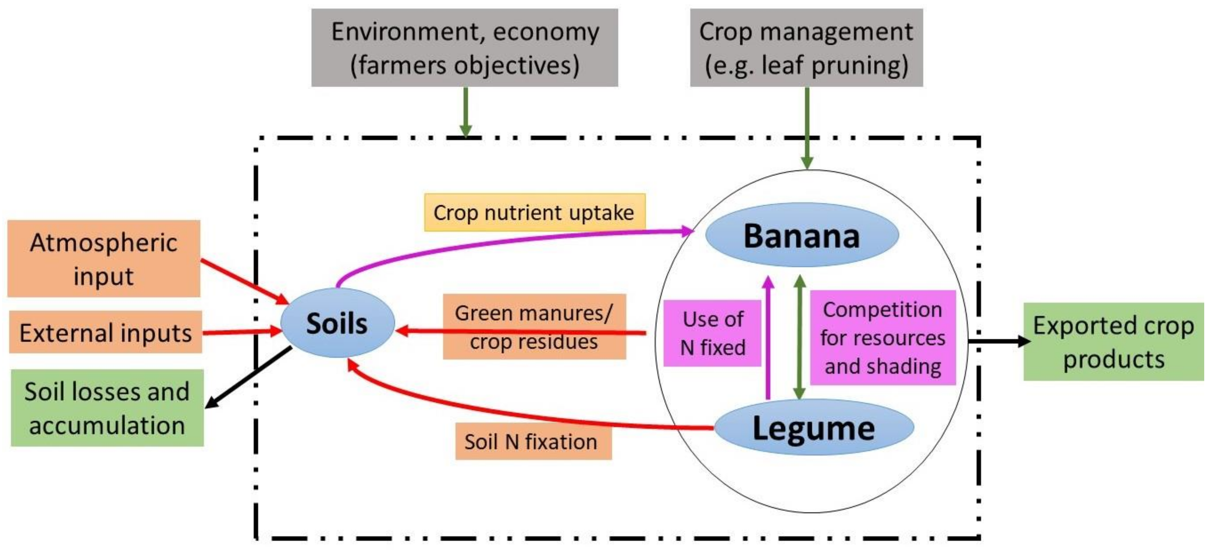
2.2. The FarmDESIGN Model

The computer-based FarmDESIGN model overcomes the limitation in comprehending complexity of farming systems by coupling a multi-objective optimization algorithm to generate a large set of Pareto-optimal alternative farm/field arrangements to a static bio-economic farm balance model that evaluates productive, economic, and environmental farm performance [39,40]. Alternatives are Pareto-optimal when they do not perform worse than any other alternatives for all the objectives [40]. The model, based on the decision variables, e.g., land allocation and management decisions, simultaneously maximizes or minimizes different objective functions to generate alternative farm configurations, making the trade-offs and synergies between objectives explicit [29]. Based on the Pareto ranking criterion [41], configurations that do not violate the constraints and perform equal to or better for at least one of the objectives (i.e., are non-dominated) are retained [40]. These configurations receive rank 1 and form the trade-off frontier. Through repeating the process, other solutions are assigned lower ranks 2, 3…, until all solutions in the set are assigned a rank (Figure 1). From the trade-off frontier solutions that perform better than the original configuration for all objectives can be assigned a superior rank “0”. The model visualizes trade-offs and synergies between the different objectives in solution spaces, leading to an increased knowledge on the interactions between the objectives and the diverse agroecosystems [40].

The FarmDESIGN model consists of a large array of various interrelated components including: The biophysical environment, socio-economic setting, crops and their products, rotations, animals and their products, on-farm produced manures, imported inputs (e.g., fertilizers, manures, herbicides), buildings, and equipment [40]. It computes farm resource flows and balances of SOM, carbon, N, P, K, and other soil nutrients through and from a farm. In addition, farm and household labor balances, household nutrition, economic results (e.g., operating profit, household budgets) are calculated on a yearly basis [34,40].

The current study is, however, based on a single field with two crop species, thus a simpler conceptual model (Figure 2) of the field was developed. This field conceptual model was comprised of the soils (biophysical environment), the two crops (banana and legume) that interacted among themselves and the management of the crops (pruning of banana leaves, intercropping or monocropping), and fields (e.g., manure application) (Figure 2). The field components are influenced by the crop management practices, the environment and socio-economic factors such as prices, input, and labor costs.

2.3. Model Inputs, Outputs and Exploration

The performance of the above field system was explored without any additional external inputs (i.e., business as usual, ‘BaU’) and with alternative improvements for addressing the soil nutrient balances. For all input scenarios, in addition to N input from farmyard manure and crop residues, symbiotic, non-symbiotic N fixation, and atmospheric N deposition were considered [42]. The different input scenarios are described below.

(i)

Business as usual (‘BaU’): This scenario benefitted only from farmyard manure applied at planting and crop residues returned to the soil. No additional external inputs were added during the three-year period of the banana crop;

(ii)

hedges (‘H’): Border/alley hedge crops rich in N and/or K were explored as an alternative for nutrient recycling within the system. The hedge species used in the model are calliandra (Calliandra calothyrsus) and tithonia (Tithonia diversifolia). Calliandra and tithonia have been reported to be good sources of N and K [43,44,45] that are often limiting in banana systems;

(iii)

inorganic input source of N, P, and K (‘I’): The model was allowed to choose between different inorganic input sources so as to bridge input gaps in the system;

(iv)

a combination of the two hedge species and inorganic input (‘H’ + ‘I’);

(v)

a combination of the two hedge species and goat manure (‘H’ + ‘M’); and

(vi)

a combination of the two hedge species, goat manure, and the inorganic inputs (‘H’ + ‘M’ + ‘I’).

The full set of objectives, decision variables, and constraints used are outlined in Table S1 and were used as described below.

Objectives: Four objectives, operating profit maximization, N input minimization, soil organic matter (SOM) balance maximization, and protein yield maximization are explored in this study. Operating profit and increasing access to protein in diets are important objectives for smallholder farmers in the study region, with beans integrated within banana primarily to meet their protein needs. Nutritional yield of proteins is determined as the number of adults that can obtain 100% of their recommended daily reference intake (DRI) per year [46] from a ha of land planted with the crop(s) of interest. SOM, N, P, and K balances are crucial for supporting the productivity of the system. For example, K and N are, respectively, required in large quantities by the banana crop [47,48].

Decision variables: The decision variables used for the explorations included land allocation to the seven banana–bush bean intercrop treatments (described in the section ‘field experiment’) and two hedge crops (calliandra and tithonia); crop product destinations; five different inorganic fertilizer options and their respective amounts; and manure from goats. The edible crop products were all assumed to be sold while crop residues were returned to the soil as mulch. The fertilizer options included NPK (17%N, 17%P and 17%K; 0.8 US$ kg⁻¹), calcium ammonium nitrate (CAN; 26%N; 0.5 US$ kg⁻¹), diammonium phosphate (DAP; 18%N, 46%P; 0.78 US$ kg⁻¹), muriate of potash (MOP; 61%K; 0.78 US$ kg⁻¹), and urea (46%N; 0.65 US$ kg⁻¹). The manure from goats (0.11 US$ kg⁻¹) is included as a cheaper alternative external source of N, P, K, and SOM. The amount of manure was varied between 0 and 8 Mg ha⁻¹. Thus, generated solutions can include various sources of nutrients, either the more expensive inorganic fertilizers and/or the cheaper manure, and/or the trimmings from hedge crops to find optimal combinations.

Constraints: Constraints were set to ensure that solutions utilized the full area and did not include combinations with worse nutrient balances of N, P, and K (Table S1). The K balance for the treatments with extreme banana leaf pruning, i.e., bananas with four leaves–bush bean intercrops (‘B4i’) that served as the starting point for all optimizations, was negative (−131 kg ha⁻¹ yr⁻¹), while the N and P balances were positive (

Table 2. The performance of seven different banana–bush bean intercrop treatment combinations for different potential production objectives (i.e., income, nutrient yield, and environmental) when each was subjected to one ha of land.

Variable	Banana Monocrop			Banana-Bush Bean Intercrop			Bush Beans (Bb)
	B9m	B7m	B4m	B9i	B7i	B4i
Operating profit (US$ ha−1 yr−1)	5482	4193	3794	5299	4471	2575	−9
N input (kg ha−1 yr−1)	161	161	161	179	185	188	211
Protein yield (persons ha−1 yr−1)	25	21	19	31	29	23	15
Soil OM balance (kg ha−1 yr−1)	15514	14942	14152	16294	16009	14962	11393
Soil K balance (kg ha−1 yr−1)	−302	−216	−189	−321	−261	−131	161
Soil N balance (kg ha−1 yr−1)	47	67	74	45	62	94	164
Soil P balance (kg ha−1 yr−1)	105	107	108	102	104	107	114

B9m, B7m, and B4m denote monocrops of banana in which all (on average 9), seven, and four fully open green leaves are retained, respectively; B9i, B7i, and B4i denote bush bean intercrops with banana having all, seven, and four fully open green leaves, respectively; and bb is a bush bean monocrop. ‘N’, ‘OM’, ‘K’, and ‘P’, respectively denote nitrogen, organic matter, potassium, and phosphorus.

). The K balance for ‘BaU’ and hedges were constrained to a minimum of −131 kg ha⁻¹ yr⁻¹, whereas for the other soil nutrient input scenarios that could offset the nutrient balances was set to be greater than 0. The total amounts of the different fertilizers applied were constrained between zero and amounts slightly above the nutrient requirement for bananas based on the main nutrient supplied by the fertilizer type. These rates were based upon recommended fertilizer rates of 100 kg ha⁻¹ yr⁻¹ of N, 30 kg ha⁻¹ yr⁻¹ of P, and 200 kg ha⁻¹ yr⁻¹ of K for East African highland bananas [49]. NPK, CAN, and urea were targeted at attainment of the soil N needs and were, respectively, allowed to vary to a maximum of 700, 400, and 300 kg ha⁻¹ yr⁻¹ of fertilizer input. DAP was aimed at P while MOP was aimed at K supply, and the two were, respectively, constrained to a maximum of 70 and 500 kg ha⁻¹ yr⁻¹ of fertilizer input.

Input data: Input data for the FarmDESIGN model were obtained from the field experiment, local markets, FarmDESIGN repository, and other secondary data. Input data obtained from the empirical experiment included crop yields (kg ha⁻¹ yr⁻¹) (Table 1); cultivation costs (combining cost of labor, seeds, and other inputs, Table 1); and the soil nutrient levels. The price of bush bean grains and bananas in the market was 1.00 US$ kg⁻¹ and 0.15 US$ kg⁻¹, respectively. Values available in FarmDESIGN and secondary literature were used for obtaining other environmental variables such as deposition and fixation of nitrogen; nitrogen, phosphorus, potassium, and dry matter content of the crop residues; and the organic matter decomposition rates. The HarvestPlus food composition table for Central and Eastern Uganda [50] and the USDA food composition table [51] were used to determine the nutritional compositions for the two crop species. Nutrient contents available in literature were used for calliandra and tithonia [44,45]. Variable yields have been reported for calliandra (7 to 55 Mg ha⁻¹; [43,52,53], and a modest yield estimate of 20 Mg ha⁻¹ was used for calliandra, while a yield of 25 Mg ha⁻¹ was used for tithonia [54]. For the goat manure, nutrient levels (1.36%N, 0.06% P and K) from on-farm experiments in Uganda [55] with similar settings to the current study area are used for the model.

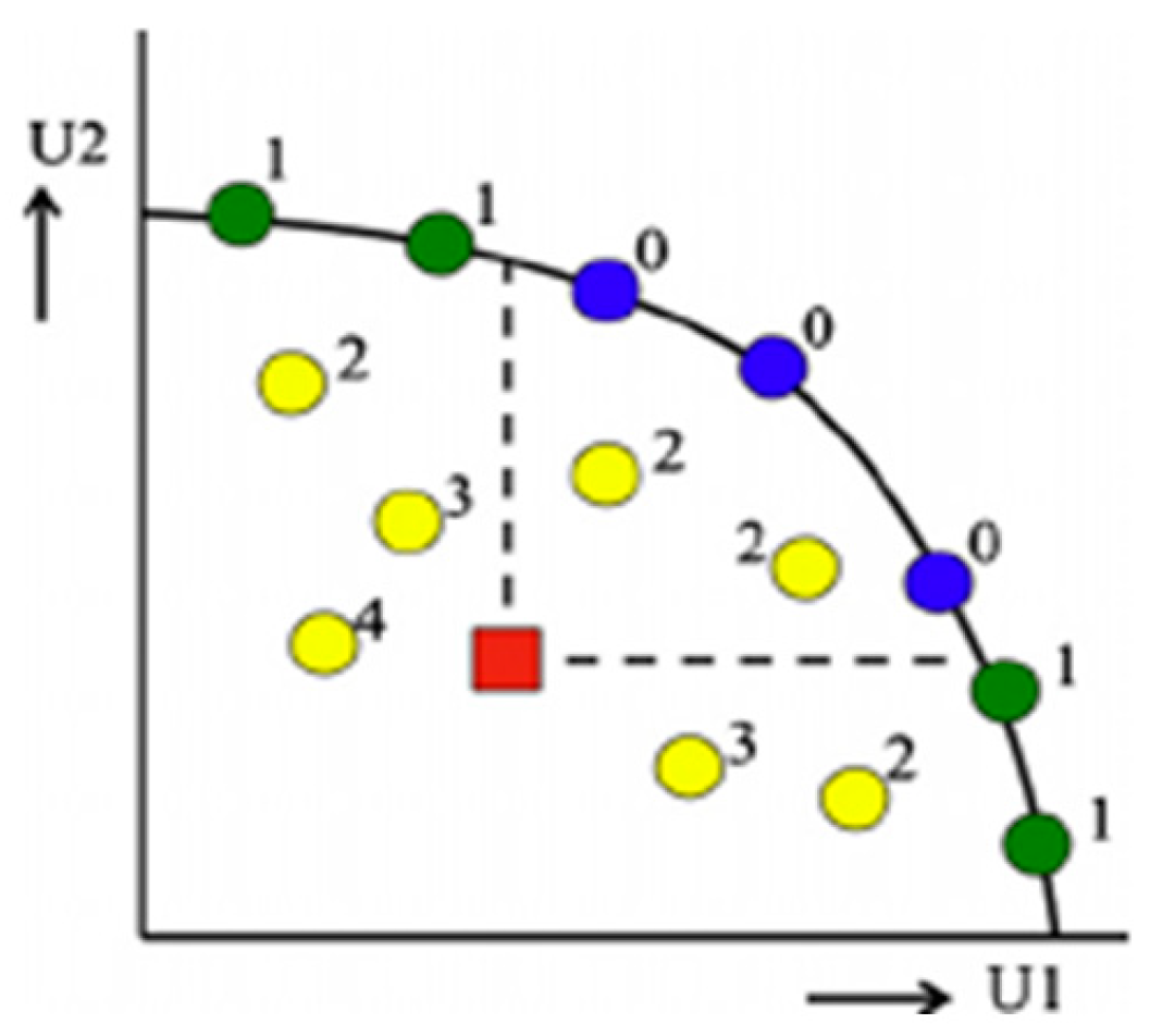
2.4. Model Exploration

In all explorations, the practice of intercropping banana plants having four leaves with bush beans (i.e., treatment ‘B4i’) served as a starting point. The model was set to generate 1000 alternative solution sets over 2000 iterations. The optimization aimed at searching for improvements relative to the current farm configuration [40]. The model simultaneously explored to achieve the set objectives. The model was separately optimized for the six scenarios; (i) ‘BaU’, (ii) ‘H’, (iii) ‘I’, (iv) ‘H’ + ‘I’, (v) ‘H’ + ‘M’, and (vi) ‘H’ + ‘M’ + ‘I’ to improve the soil nutrient balances. The model outcomes (solution spaces) from the different runs were compared with each other. From the solution spaces, Pareto-frontier configurations that performed better than the original configuration for pairs of objectives (marked “0” in Figure 1 above) were examined and plotted to simplify the output and to make the trade-offs and synergies between the objectives explicit. The model trends were also examined for the allocation of land to the treatments and hedges with respect to the objectives.

3. Results

3.1. Treatment Comparisons Prior to Exploration

Table 2 shows a comparison of the seven banana-bush bean intercrop treatments for ‘BaU’ prior to optimization. As expected, the highest N input was obtained in the legume plot followed by the intercrops, with N input in the intercrops increasing with leaf pruning levels. N balances were higher in the bush beans followed by the banana with four leaves–bush bean intercrop. N balances generally increased with the leaf pruning levels for both the intercrops and sole banana crop. Lower balances occurred for intercrops in which seven and all leaves had been retained compared to their corresponding monocrops. Soil K balances were only positive for the bush bean monocrop (‘Bb’). Higher protein yield and SOM balance occur for the intercrops, though this declines with subsequent leaf pruning levels. In contrast, the sole banana crops outperform the intercrops in terms of operating profit, suggesting a trade-off with N input, protein yield, and SOM balance.

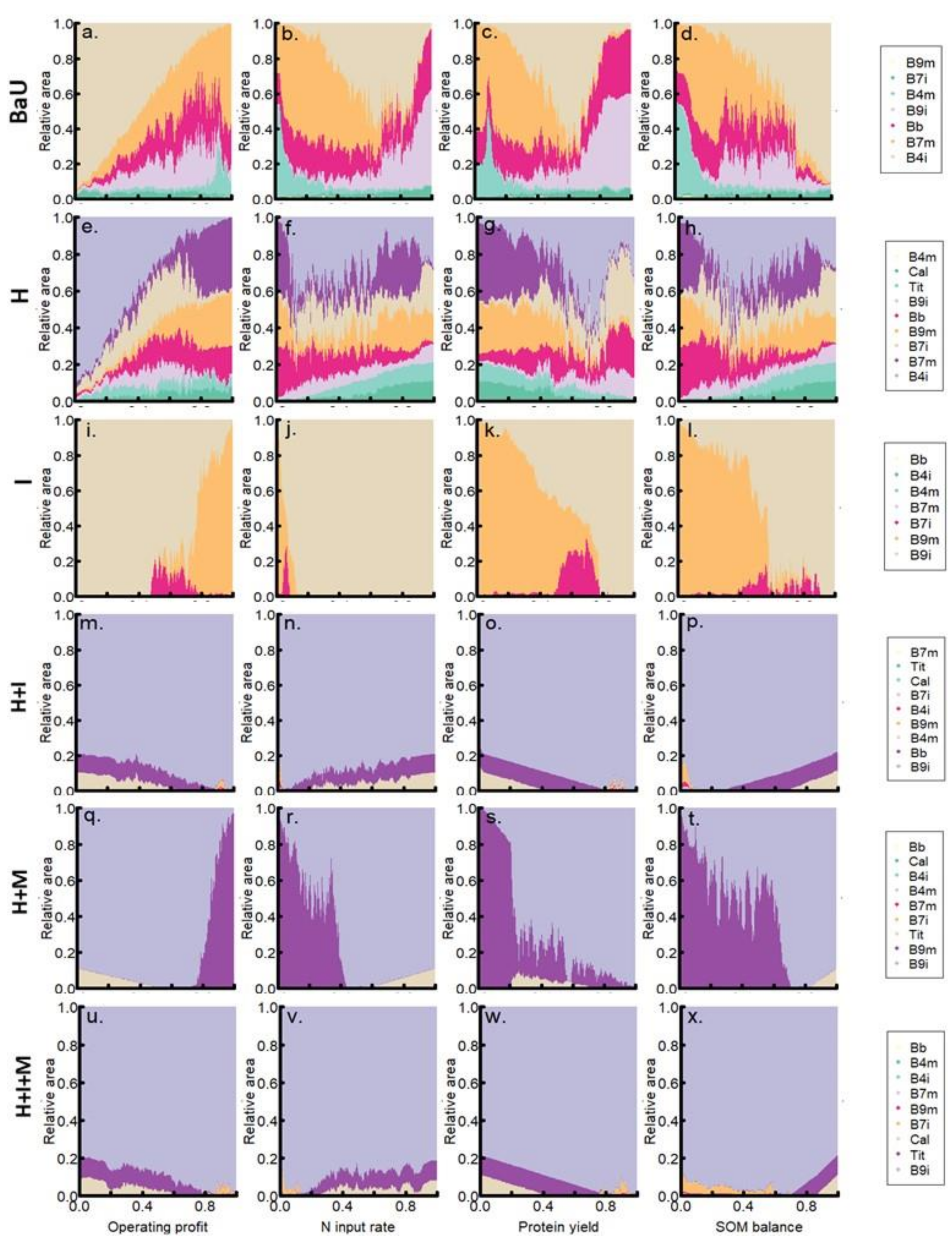
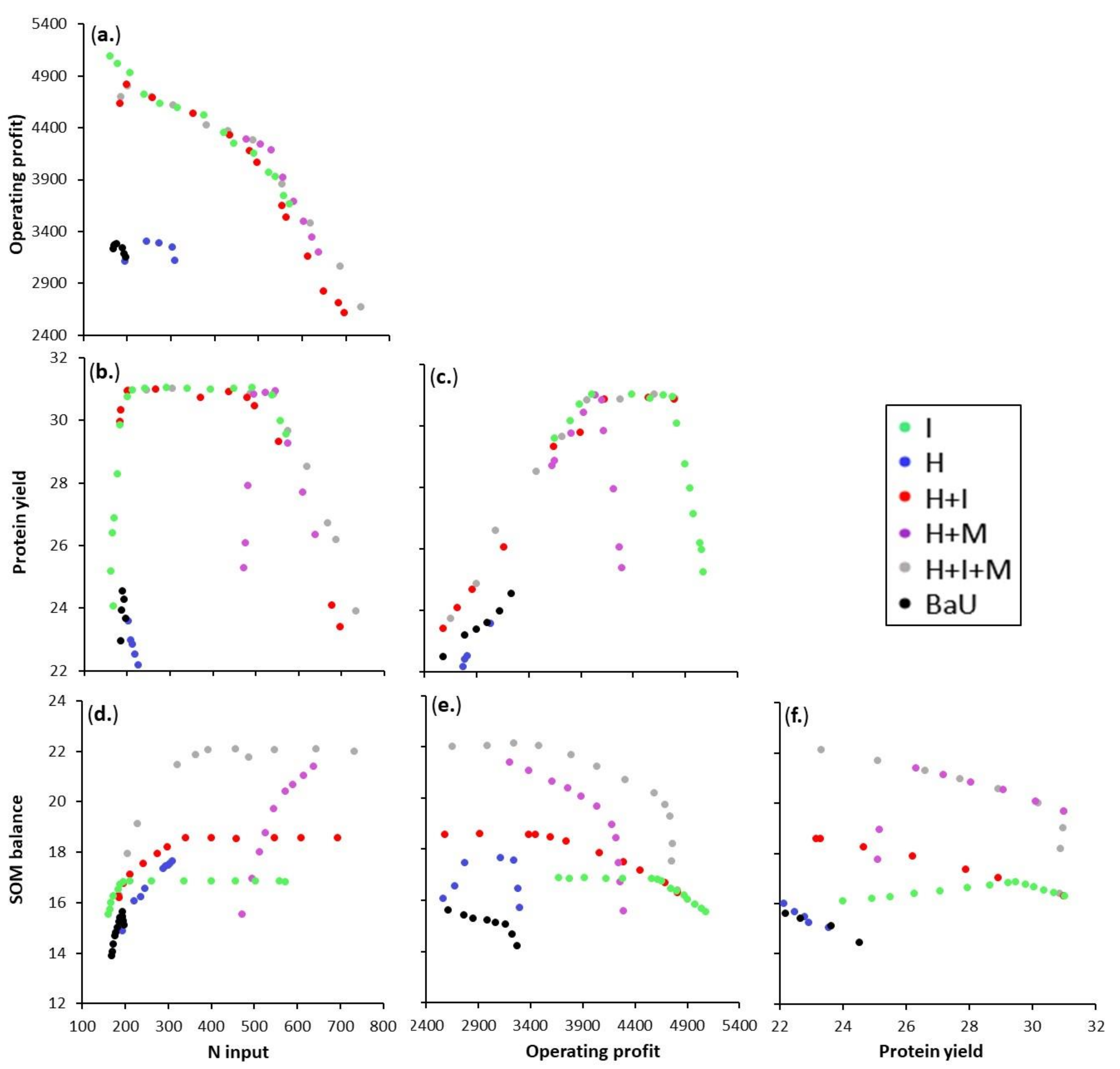
3.2. Banana–Bush Bean Intercrop Model Explorations with Different Input Scenarios

Model exploration for the scenario business as usual (‘BaU’, without extra inputs) resulted in configurations that are superior to the original field configuration (legume intercropped with bananas having four leaves) only for operating profit and N input (Figure 3). Lower performances relative to the original field configuration are observed for protein yield and the SOM balance (Figure 3b–f). Soil K balance was also negative for the system. Thus, improvements in the system for these objectives and K balance are not feasible and viable through only re-arranging the field components as in ‘BaU’. Compared to other scenarios, ‘BaU’ had the lowest levels for N input, and this could have limited model explorations.

Profound improvements in model explorations and overall performance of production objectives compared to ‘BaU’ occurred across all the input scenarios, except for the use of hedges (‘H’) (Figure 3). The ‘BaU’ and ‘H’ scenarios had small clouds of solution sets, with the hedges often performing more poorly than ‘BaU’ for some objectives (Figure 3,

Table 3. The range of the different production objectives achieved in the exploration using various scenarios for soil nutrient improvement in a banana–bush bean intercrop in eastern DR Congo.

Input Scenarios	N Input (kg ha−1 yr−1)		Operating Profit (US$ ha−1 yr−1)		Protein Yield (Persons ha−1 yr−1)		SOM Balance (kg ha−1 yr−1)
	Min	Max	Min	Max	Min	Max	Min	Max
BaU	170	199	2575	3279	18	25	13875	15604
H	176	318	2524	3385	17	24	14147	17957
I	162	574	1403	5085	23	31	14962	16851
H + I	185	697	1403	4811	23	31	14962	18585
H + M	474	640	1321	4298	23	31	15534	21373
H + I + M	186	735	1321	4810	23	31	13875	22116

BaU = Business as usual (i.e., no additional external inputs), H = hedges, I = inorganic fertilizer and M = goat manure.

). Overall, scenarios with inorganic input performed better for operating profit, protein yield, and N input, while those with manure had the highest yields for SOM balance. For example, the maximum operating profits varied between 4810 and 5085 US$ ha⁻¹ yr⁻¹ for input scenarios with inorganic fertilizers compared with 3279 US$ for ‘BaU’, 3385 US$ for hedges only, and 4298 US$ for the combination of hedges and manure (Table 3). The minimum N inputs varied between 162–186 kg for inorganic inputs compared with 170, 176, and 474 kg for ‘BaU’, hedges, and hedges with manure, respectively. The combination of hedges with manure generally had the greatest N input. With exception of ‘BaU’ and ‘H’ (protein yield between 17 and 25 persons ha⁻¹ yr⁻¹), protein yield increased to a maximum of 31 persons ha⁻¹ yr⁻¹ from 23 persons ha⁻¹ yr⁻¹ (Figure 3b,c,e; Table 3). Zones of trade-offs and synergies were visible in the clouds and frontiers of the alternative solutions across the different scenarios. For ‘BaU’ and ‘H’, where the supply of soil nutrients is low or limiting, the model appears to include more diversity of land uses, while less diverse solutions are generated for the other input scenarios (Figure 4).

3.2.1. Operating Profit

For the ‘BaU’ and hedge (‘H’) scenarios, low operating profit is associated with a higher relative area for bananas having four leaves–bush bean intercrop (‘B4i’) (Figure 4a,e), while land was predominantly allocated to the intercrop bananas having all leaves retained with bush beans (‘B9i’) for the other input scenarios (Figure 4i,m,q,u). At high operating profit levels, the model allocated land to a combination of banana with seven leaves monocrop (‘B7m’), bush bean monocrop (‘Bb’), and ‘B9i’ for the ‘BaU’ scenario (Figure 4a), whereas it was to ‘B7m’, ‘B9m’ (banana-all leaves monocrop), and ‘Bb’ for the ‘H’ scenario (Figure 4e). For the inorganic input (‘I’, Figure 4i) and combination of ‘H’ with goat manure (‘M’) (Figure 4q), the model increased land allocation to ‘B9m’, while for scenarios combining ‘H’ with ‘I’ (Figure 4m) and ‘H’, ‘M’, and ‘I’ (Figure 4u), the share for ‘B9i’ increased with increasing operating profit. For ‘H’ + ‘I’ and ‘H’ + ‘I’ + ‘M’, low amounts of calliandra (‘Cal’) and tithonia (‘Tit’) hedges are observed at lower levels of operating profit.

3.2.2. N Input

A low N input for the ‘BaU’ scenario was mainly associated with sole banana crops with seven (‘B7m’) or four (‘B4m’) leaves (Figure 4b). In contrast, a higher relative land area was allocated to ‘B7m’, ‘B9m’, and ‘Bb’ for the ‘H’ scenario (Figure 4f), ‘B9m’ and ‘B9i’ for the ‘I’ (Figure 4j) and ‘H’ + ‘M’ (Figure 4r) scenarios. The ‘H’ + ‘I’ and ‘H’ + ‘I’ + ‘M’ scenarios had a high land allocation to ‘B9i’ (Figure 4n,v). At high N input, ‘BaU’ was mainly associated with ‘Bb’ and ‘B9i’, ‘H’ with ‘B4i’, ‘B7i’ (intercrop of banana having seven leaves with bush beans), and ‘Bb’, and ‘B9i’ was associated with scenarios that had I as one of the input options.

3.2.3. Protein Yield

Land allocation with protein yield varied across the input scenarios. A low protein yield was predominantly associated with treatment ‘B7m’ in ‘BaU’ (Figure 4c), and ‘B7m’ and ‘B9m’ for ‘H’ (Figure 4g). For ‘I’ and the combination of ‘H’ with ‘M’ (Figure 4k,s), a low protein yield was mainly associated to the banana monocrop ‘B9m’, while the remaining scenarios (Figure 4o,w) were mainly associated with ‘B9i’. At high protein yield, large allocations to the bush bean monocrop (‘Bb’) occurred for scenarios ‘BaU’ (Figure 4c) and hedges (Figure 4g). Treatments ‘B9i’ for ‘BaU’ and ‘B4i’ and ‘B7i’ for hedges were also important for a high protein yield. In contrast, ‘B9i’ predominates for the other input scenarios at high protein yield (Figure 4k,o,s,w).

3.2.4. Soil Organic Matter (SOM) Balance

For the scenario ‘BaU’, a low SOM balance was associated to treatments ‘B7m’, ‘B7i’, and ‘Bb’ (Figure 4d) while to treatments ‘B7m’, ‘Bb’, and ‘B9m’ for the ‘H’ scenario (Figure 4h). For the ‘I’ (Figure 4l) and ‘H’ + ‘M’ combination (Figure 4t), more land was allocated to ‘B9m’ at a low SOM balance, while it was allocated to ‘B9i’ for ‘I’ + ‘H’ (Figure 4p) and ‘H’ + ‘M’ (Figure 4t). At high SOM balance, most of the land is allocated to ‘B4i’ for ‘BaU’ (Figure 4d), a combination of ‘B4i’, ‘B7i’, and ‘B9m’ for hedges (Figure 4h), and ‘B9i’ for other scenarios (Figure 4l,p,t,x).

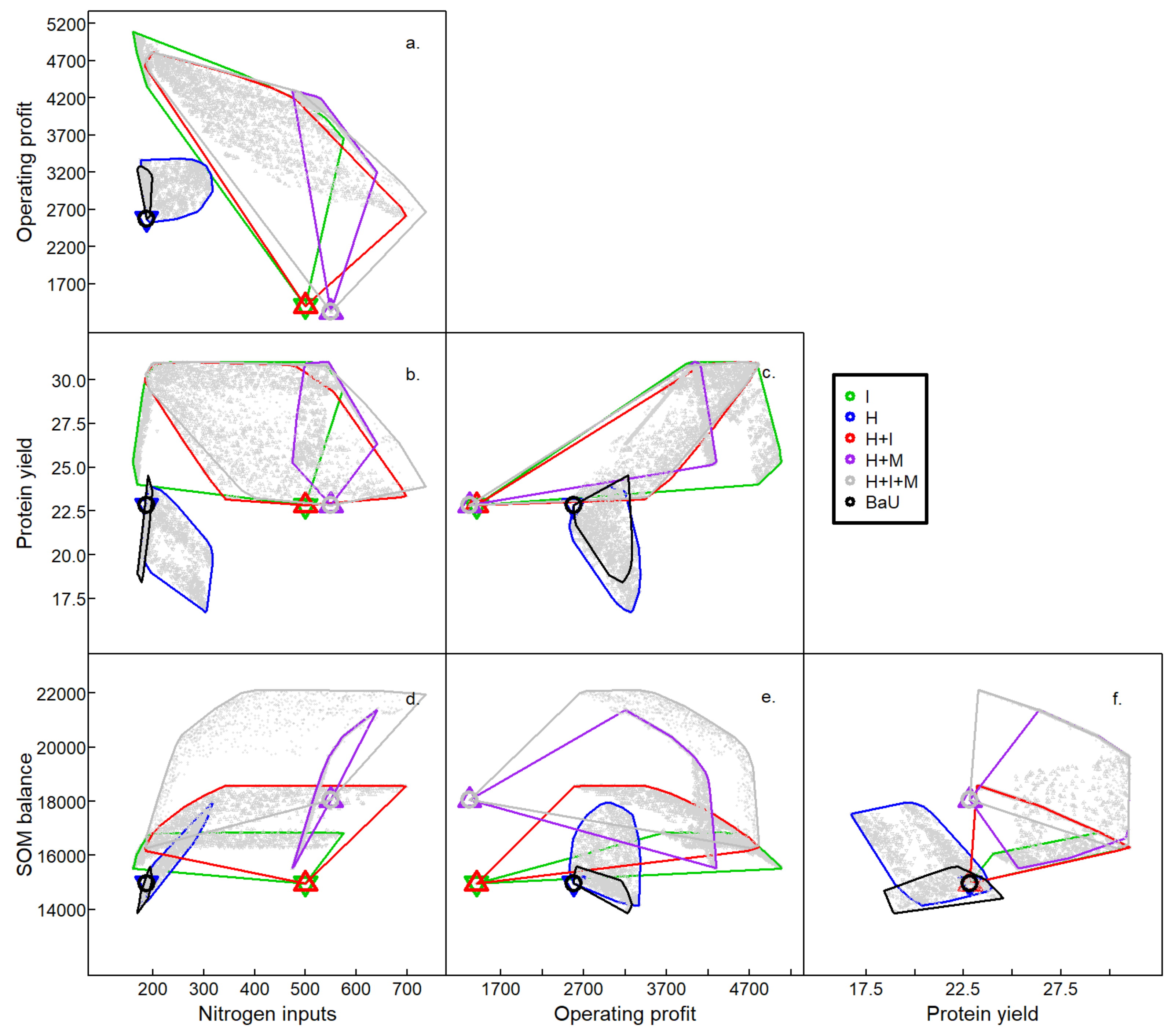
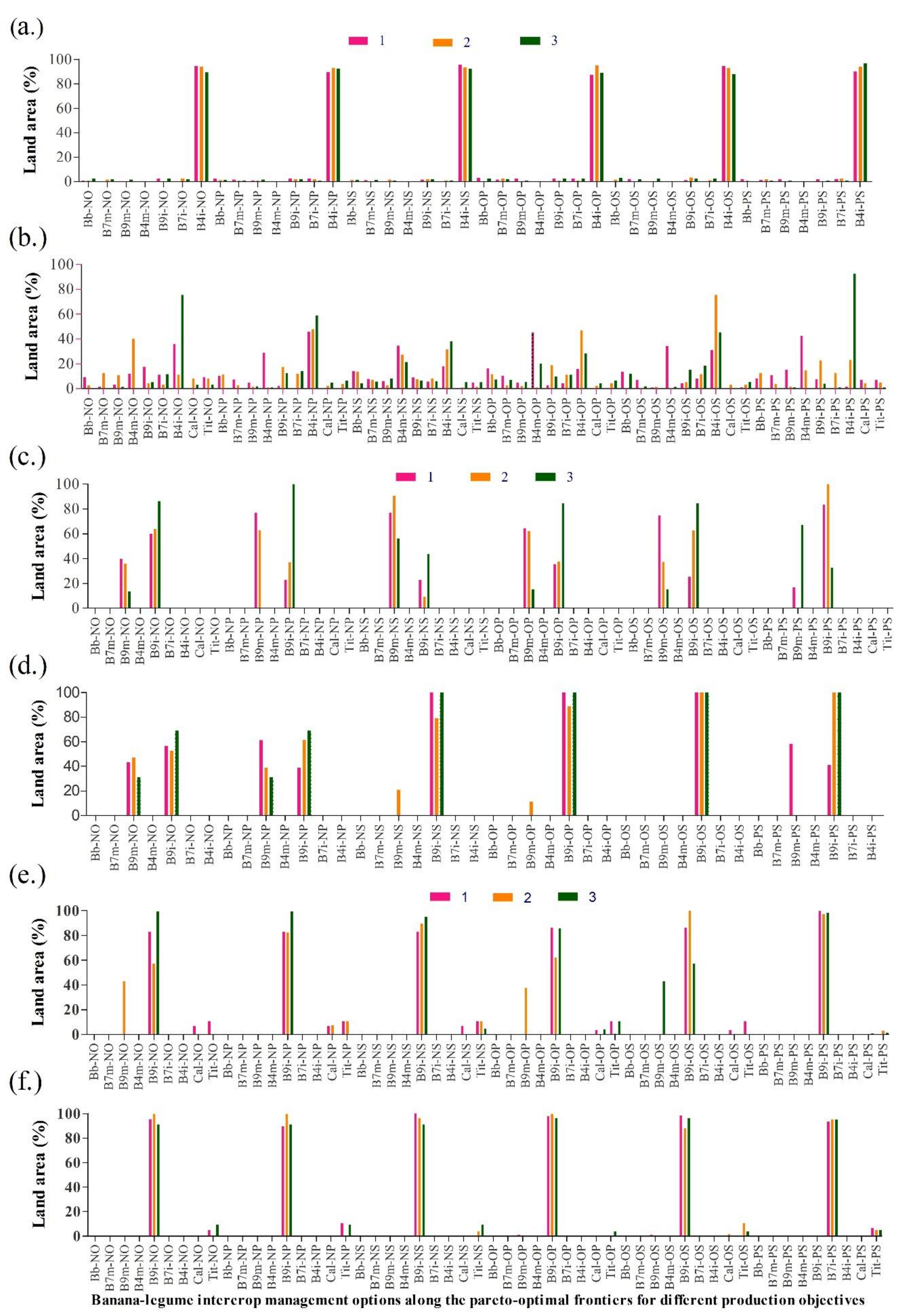
3.3. Pareto-Frontier Trade-Offs and Synergies between Production Objectives

Figure 5 presents the relationship at the Pareto frontier, i.e., ranks “0” and “1” in Figure 1, between the four production objectives, i.e., minimization of N input, maximization of operating profit, protein yield, and SOM balance. Apart from the interaction between N input and SOM balance in which a more synergistic relation occurred, zones of trade-offs and synergies were both visible for the interactions between the remaining objectives (Figure 5). The ‘BaU’ and hedge scenarios consistently had a smaller window of opportunity for exploration, resulting in smaller solution spaces and dismal levels of operating profit, protein yields, and SOM balance (Figure 3a, Figure 5a–f). A moderate performance was observed for a mixture of hedges with goat manure while options with inorganic fertilizer as a nutrient source had larger solution spaces and more robust increases in operating profit, protein yield, and SOM balance. N input, that was minimized, was relatively low (170–198 kg ha⁻¹ y⁻¹) at the Pareto frontier for the ‘BaU’ scenario and moderate (196–311 kg ha⁻¹ y⁻¹) when hedges were used for supplementing nutrients. N input for the inorganic input varied between 161 and 558 kg ha⁻¹ y⁻¹. Goat manure had the worst performance for N input (that was minimized), with high N input values varying between 473 and 639 kg ha⁻¹ y⁻¹.

Figure 6 shows the allocation of land for different field management scenarios at 3 points (left, middle, and right) along the rank “0” Pareto frontiers of the plots in Figure 5. Solutions along the rank “0” Pareto frontier outperform the original farm configuration for all production objectives. The allocation of land between the treatments/management options along the rank “0” Pareto optimal frontier profoundly differed from one input scenario to another for the interactions between the four-production objectives. For the ‘BaU’ scenario, the model predominantly allocated the available land (87–97%) to cultivation of an “intercrop of the severely pruned banana crop with bush beans” at the rank “0” Pareto frontier of the interactions between all the production objectives (Figure 6a). In the hedge-only scenario, land was split up between a range of treatments, with the largest allocation to the “intercrop of severely pruned banana crop with bush beans” (Figure 6b). When hedge plus goat manure (Figure 6c) or inorganic fertilizer (Figure 6d) is used, the model predominantly allocates land to a combination of an “un-pruned banana monocrop” and “un-pruned banana–bush bean intercrop” at the rank “0” Pareto frontier across all objectives. Differences in the levels of land allocated to the treatments are, however, observed between the production objectives for the two input scenarios. For example, for the interaction between N input and SOM balance (‘NS’ in Figure 6), 56–91% was allocated to “un-pruned banana monocrop” for the hedge–goat manure input scenario compared with 79–100% to the “un-pruned banana–bush bean intercrop” for the inorganic input scenario. The model did not allocate land to any of the hedges, in the hedge–goat manure scenario. For the hedge–inorganic fertilizer (Figure 6e) and hedge–goat manure–inorganic fertilizer (Figure 6f), respectively, 57–100% and 88–100% of land was assigned to “un-pruned banana–bush bean intercrop” across the production objectives.

4. Discussion

The FarmDESIGN model has been used to unravel complexities at farm level through the determining of trade-offs and synergies between farm objectives and exploring windows of opportunities for improving farm performance. In the current study, the model was applied at field level to address complexities associated with the management and the interaction in a banana–bush bean intercrop. Complexities in this system arise from the difficulties in measuring environment and nutrition related objectives that are often subtle to farmers and seldom a concern. The computer based FarmDESIGN model explored the trade-offs and synergies for alternative banana–bush bean intensification/management options as a basis for identifying the most economically viable and environmentally sound management alternatives. The model also explored different input scenarios for addressing soil infertility, a major limitation of banana production systems in the AGLR.

The pruning of banana leaves to integrate legumes profoundly reduced the operating profit and SOM balance of the system, whereas N input in the system reduced with increasing leaf pruning. Reduction in operating profit and SOM balances with increased leaf pruning can be attributed to the reduced photosynthetic capacity that affects overall growth and development and fruit filling. Leaf area of the banana crop has been reported to be positively correlated to bunch weight and overall performance of the crop [56,57]. Ocimati et al. [18] reported leaf cutting to integrate legumes to result in an economically inefficient system despite a higher agronomic efficiency for a moderately pruned banana crop. An increase in N input with increasing levels of leaf pruning can be attributed to (i) increased vigor of the bush bean due to higher access to light and higher biological nitrogen fixation, and (ii) a reduction in nutrient uptake/demand with increasing banana leaf pruning levels. A profound reduction in root growth and nodulation with a subsequent depression in biological N fixation in legume spp. has been reported due to shading [58,59,60]. Bloom et al. [58] reported a higher allocation of dry matter to shoots when light is limited, leading to poor root and nodule development. The reduced uptake by the banana crop can be attributed to a reduced root mass associated with leaf pruning [61]. This is further supported by the fact that the N, P, and K balances in the soil increased with increasing leaf pruning levels.

Model exploration without extra inputs (‘BaU’), i.e., re-arranging the field components alone and addition of hedges only offered a smaller solution space for improving the performance of the banana system in the studied farm for most objectives. In contrast, explorations with scenarios that included the addition of inorganic fertilizer and goat manure profoundly improved the performance of the system for most of the objectives explored. This suggests that soil nutrients are a major limiting factor for the banana–bush bean system. The dismal performance of hedges is possibly because they mainly help in nutrient recycling [62]. Furthermore, hedges reduced the total area that could be allotted to the banana and the legume crop. The scenarios with inorganic N, P, and K sources outperformed the other input scenarios for operating profit (maximized), protein yield (maximized), and N input (minimized). This can be attributed to a relatively lower cost of, and the ease to adequately fulfil, the multiple nutrient requirements of the system through the inorganic sources. In contrast, goat manure led to a very high N input and SOM balance. The goat manure had a low K content (i.e., 0.06%). Soil K is the most limiting nutrient for banana production [47,48] and the east African highland bananas are, for example, reported to be more sensitive to potassium deficiency than other factors [48]. Thus, large amounts of goat manure are needed to bring soil K to sufficient levels, leading to above optimal levels of N input. In/contrast, the amount of carbon in the goat manure was high. The N input ranges for all the input scenarios (162–735 kg ha⁻¹ yr⁻¹) were higher than the recommended blanket rate (i.e., 100 kg ha⁻¹) for east African highland banana systems in Uganda [63] but are in agreement with recommendations for high yielding banana plantations (i.e., 300–450 kg N ha⁻¹) elsewhere [64,65]. More recent studies (e.g., [47,48]) show better responses of the east African highland banana to higher levels of N, P, and K (i.e., 150–400 N, 50 P, and 250–600 K). The N input values from the FarmDESIGN model in this study are thus within the acceptable range for the banana crop.

Land allocations to treatments across the input scenarios were strongly influenced by the availability of soil nutrients and the nutrient demand of the crops. For the ‘BaU’ scenario, when all solution spaces are considered, a combination of treatments were selected, with a higher allocation to the “severely pruned banana–bush bean intercrop”, and “sole bush bean crop” at lower operating profits, while a “moderately pruned banana–bush intercrop” and/or “un-pruned banana–bush bean intercrop” at high profitability (c.f. Figure 4). This corroborates the findings of [18] that recommended intercropping bush beans within moderately pruned and un-pruned banana plants based on their high agronomic and economic efficiencies. However, the rank “0” Pareto frontier solutions in the ‘BaU’ input scenario (c.f. Figure 6) were dominated by the severely pruned banana–bush bean intercrop, suggesting that more profitable options such as moderately- or un-pruned banana intercrop with bush beans to either be unsustainable without the addition of external inputs. It is important to note that, unlike [18], who based their conclusions on the agronomic/economic efficiency only, the current study sought to optimally and simultaneously address multiple (i.e., economic, nutrition, and environment) production objectives. The selection of the “severely pruned banana crop” at the rank “0” Pareto frontier as described above, is potentially because of the low nutrient uptake arising from a reduced banana root mass. In contrast, a sole un-pruned banana as a monocrop or intercrop would demand a higher amount of nutrients, resulting in a more rapid soil nutrient depletion and in the long run a total collapse of the system in the absence of external nutrient addition. Improving the performance of the banana systems will thus necessitate the addition of external input.

The hedge scenario also had a similar distribution of treatments when all solution spaces were considered. However, unlike ‘BaU’ that had land predominantly allocated to the “intercrop of severely pruned banana and bush beans” at the rank “0” Pareto frontier, the hedge scenario had land allocated to multiple treatments including “moderately pruned and un-pruned banana intercrop with bush beans”. This suggests an increased availability of inputs, arising from the recycling of the pruned hedge biomass and N-fixed by the hedges. Hedges could thus potentially improve nutrient balances on smallholder farms. Planting hedges along the boundaries of homesteads to secure and beautify homes and around fields/farms as demarcations is a common practice in the study region. Nitrogen fixing and N-rich hedges with high biomass production ability have been reported to potentially improve soil fertility [62,66]. These hedges could also be a good source of fodder for integrating zero-grazed livestock; and improving on-farm nutrient recycling on smallholder farms. They can also be used as mulch or green manure, reducing wind and water erosion on these smallholder farms. Hedges are also known to harbor natural enemies of crop pests and increase agrobiodiversity within farms [67]. Calliandra is reported to be beneficial for rehabilitation of erosion-prone areas and lands exhausted by agriculture, providing shade for other partially shade-tolerant trees and crops, fixing N through its symbiotic Rhizobium bacteria and root fungus, and improving soil through its high N-rich leaf biomass yields and well-developed lateral rooting system [43]. It is reported to be compatible with crops having both extensive fibrous roots and deep roots, thus being suitable for hedgerow boundaries [43]. Positive effects of tithonia on subsequent rice and maize crops have also been reported [68]. Tithonia is common in the study region, growing wildly, as a hedge or weed on farms. Enlightening farmers on the potential benefits of hedges could increase their role in nutrient recycling within these production systems.

The scenarios that supplemented nutrients through the addition of inorganic fertilizers, goat manure, or a mixture of both predominantly allocated land to the “intercrop of un-pruned” and/or “a sole un-pruned banana crop with bush beans”. This contrasts with the ‘BaU’ and hedge scenarios, in which solutions with “severely pruned banana–bush bean intercrop” dominated. This supports the fact that nutrient availability is a major constraint to the banana intercrops systems in the study region. This further suggests that improving the performance of the banana intercrops systems in the region requires a judicious investment in external inputs

Trade-offs and synergies were visible between the objectives at the Pareto-optimal frontiers. Synergies occurred between N input and operating profit, suggesting that both could be improved simultaneously. Synergies were also observed for operating profit and protein yield when input scenarios contained hedges. The observed synergies could be attributed model limitations discussed below. Trade-offs were profoundly visible between the other interactions of the objectives. Strategies to manage these trade-offs will be crucial and may be more dependent on farmers priorities and access to resources. For example, a resource-endowed, market-oriented farmer may be willing to invest more in external inputs to increase his profitability, with the contrary holding true when a farmer is producing predominantly for home consumption.

The FarmDESIGN model improved the robustness of the empirical experiment and unraveled the relations between production objectives (i.e., operating profit, N input, protein yield, and SOM balances), constraints, and decision variables, which would have been challenging to explore using the empirical experiment only. The model generated numerous rank “0” Pareto-optimal alternative farm configurations with varying input and output (i.e., outcomes of the production objectives) combinations, giving a large set of alternatives that farmers can choose from. It also made the synergies and trade-offs between the objectives explicit. Knowledge of the trade-offs and synergies with environmental and nutritional objectives are especially very crucial given that they are often ignored or unknown to farmers and difficult to measure. The model could thus be useful in facilitating discussions between extension and/or research staff with farming communities to support and improve farm decision making with respect to achieving different farm objectives within production constraints. However, the high variability within farms in terms of access to land, inputs, and other production resources; environmental and socio-economic conditions and production objectives could limit or complicate the uptake of model outcomes in this study. To overcome this, grouping farms within landscapes into more homogenous groups based on the above variabilities will be helpful for targeting and tailoring model outcomes. This grouping can also take into perspective other potential production constraints such as access to labor, inputs, and farmer production objectives. For the banana intercrop system, gender roles, especially ownership and decision making with respect to the component crops, could also hinder the implementation of model outcomes. For example, in eastern DR Congo where this study was conducted, women are responsible for the cultivation of the legume components under banana, grown mainly to meet food security and nutrition needs within the household, whereas men are often responsible for the banana crop that is often grown mainly for income. Implementation of model outcomes will thus require mutual decision making and agreements within households with respect to management of the intercrops and use of the returns from the crops. Successful model implementation at both the household and community level will thus require co-redesigning of the systems with several iterations with all the relevant stakeholders, especially the farmers and extension staff. Co-redesigning will ensure relevance of the redesigns and foster ownership, adoption, and success of model outcomes. The model also has a high input data demand. On smallholder farms, the accuracy of model outcomes could be hampered by the poor culture of record keeping. Strategies for improving data collection on smallholder farms and subsequent storage will thus be crucial for supporting decision making based on this and other similar tools. Available literature and databases, e.g., on nutrient composition tables [50,51], are also suitable inputs sources for the FarmDESIGN model. Important to note is that the FarmDESIGN model is static, and as such, does not automatically adapt crop yields to management practices like increased fertilizer levels [40]. The model thus did not reflect potential yield increases and the accompanying potential incomes that could have arisen from the improved soil nutrient balances associated with the input scenarios in this study. Factoring nutrient response curves to capture the effect of fertilizers through linking the model to existing algorithms for nutrient responses is recommended for more robust outcomes.

5. Conclusions

Severe pruning of banana leaves (e.g., to four leaves) is a common practice on smallholder farms aimed at using the limiting land to intercrop shade-sensitive crops to meet income and nutritional needs. This study has shown that severe banana leaf pruning reduces profitability, which is one of the primary production objectives of smallholder banana farmers in the AGLR. An intercrop of either moderately pruned or un-pruned bananas with bush beans is more profitable, but not optimal for multiple production objectives, especially the environmental objectives. Improvements in banana–bush bean intercrop systems are stifled, resulting in lower profitability, protein yield, and SOM balance when no or limited external inputs are added. For example, in the absence of additional external nutrient inputs (i.e., ‘BaU’ scenario), the intercrop of the “severely pruned banana crop with bush beans” is predominantly picked at the rank “0” Pareto frontier as the superior/optimal solution set for all production objectives, despite being less profitable. Minor improvements occur when hedges are introduced. Profound improvements with wider solution spaces occur when external nutrient inputs (inorganic and organic fertilizers) are used, allowing for the more nutrient demanding un-pruned banana crop in a sole or intercrop state to be grown with improvements in performance of multiple production objectives. Thus, the addition of external inputs is crucial for improving the performance of the banana intercrop systems for all objectives sustainably. Nitrogen fixing fast-growing hedges could form a good bridge between the ‘BaU’ and the input dense scenarios for the resource constrained farmers. The FarmDESIGN model was very suitable for: Exploring trade-offs and synergies between the objectives; and identifying Pareto-optimal field configurations for the banana–bush bean intercrop system. The model also supported the exploration of alternative input scenarios. FarmDESIGN model is therefore a useful tool and could be widely promoted to support decision making at field level for complex intercrop systems.

References

1. FAO. 2018. Available online: http://faostat3.ao.org/browse/Q/*/E (accessed on 22 March 2018).
2. Abele, S.; Twine, E.; Legg, C. Food Security in Eastern Africa and the Great Lakes. Crop Crisis Control Project Final Report to USAID. 2007, p. 110. Available online: http://c3project.iita.org/Doc/Final%20report%20C3P%20small.pdf (accessed on 18 March 2015).
3. Karamura, E.B.; Turyagyenda, F.L.; Tinzaara, W.; Blomme, G.; Molina, A.; Markham, R. Xanthomonas Wilt (Xanthomonas Campestris pv. Musacearum) of Bananas in East and Central Africa. Diagnostic and Management Guide; Fountain Publishers: Kampala, Uganda, 2008. [Google Scholar]
4. The World Bank Group. The World Bank Data. 2019. Available online: https://data.worldbank.org (accessed on 15 March 2019).
5. Jagwe, J.; Ouma, E.; van Asten, P.; Abele, S. Banana Marketing in Rwanda, Burundi and South Kivu CIALCA Project Survey Report. 2014. Available online: https://test.cialca.org/wp-content/uploads/2018/06/6.-Banana_market_report.pdf (accessed on 15 January 2019).
6. FAO. FAPDA Country Fact Sheet on Food and Agriculture Policy Trends—BURUNDI. 2015. Available online: http://www.fao.org/3/a-i4909e.pdf (accessed on 15 March 2018).
7. IFAD. The Democratic Republic of Congo. 2018. Available online: https://www.ifad.org/en/web/operations/country/id/dr_congo#anchor-3 (accessed on 17 January 2019).
8. Uganda Investment Authority. Agriculture. 2018. Available online: https://www.ugandainvest.go.ug/projects/ (accessed on 15 March 2019).
9. Tinzaara, W.; Stoian, D.; Ocimati, W.; Kikulwe, E.; Otieno, G.; Blomme, G. Challenges and Opportunities for Smallholders in Banana Value Chains. In Achieving Sustainable Cultivation of Banana; Burleigh Dodds Science Publishing: Cambridge, UK, 2018; pp. 85–110. [Google Scholar]
10. Sunday, G.; Ocen, D. Fertilizer Consumption and Fertilizer Use by Crop in Uganda. 2015. Available online: http://www.africafertilizer.org/wp-content/uploads/2017/05/FUBC-Uganda-final-report-2015.pdf (accessed on 15 March 2019).
11. Nandwa, S.M.; Bekunda, M.A. Research on nutrient flows in east and Southern Africa: State-of-the-art. Agric. Ecosyst. Environ. 1998, 71, 5–18. [Google Scholar] [CrossRef]
12. Ocimati, W.; Karamura, D.; Rutikanga, A.; Sivirihauma, C.; Ndungo, V.; Ntamwira, J.; Blomme, G. Agronomic practices for Musa across different agro-ecological zones in Burundi, Eastern Democratic Republic of Congo and Rwanda. In Banana Systems in the Humid Highlands of Sub-Saharan Africa: Enhancing Resilience and Productivity; Blomme, G., Vanlauwe, B., van Asten, P., Eds.; CAB International: Wallingford, UK, 2013; pp. 175–190. [Google Scholar]
13. van Asten, P.J.A.; Gold, C.S.; Okech, S.H.O.; Gaidashova, S.V.; Tushemereirwe, W.; De Waele, D. Soil quality problems in East African banana systems and their relation with other yield loss factors. InfoMusa 2004, 13, 20–25. [Google Scholar]
14. Ntamwira, J.; Pypers, P.; Van, A.P.; Vanlauwe, B.; Ruhigwa, B.; Lepoint, P.; Dheda, B.; Monde, T.; Kamira, M.; Blomme, G.; et al. Effect of banana leaf pruning on banana and legume yield under intercropping in farmers’ fields in eastern Democratic Republic of Congo. J. Hortic. For. 2014, 6, 72–80. [Google Scholar] [CrossRef]
15. Blomme, G.; Ocimati, W.; Groot, J.; Ntamwira, J.; Bahati, L.; Kantungeko, D.; Remans, R.; Tittonell, P. Agroecological integration of shade- and drought-tolerant food/feed crops for year-round productivity in banana-based systems under rain-fed conditions in Central Africa. Acta Hortic. 2018, 1196, 41–54. [Google Scholar] [CrossRef]
16. Wortmann, C.S.; Sengooba, T.; Kyamanywa, S. Banana and Bean Intercropping: Factors Affecting Bean Yield and Land Use Efficiency. Exp. Agric. 1992, 28, 287–294. [Google Scholar] [CrossRef]
17. Ouma, G. Intercropping and its application to banana production in East Africa: A review. J. Plant Breed. Crop Sci. 2009, 1, 13–15. [Google Scholar]
18. Ocimati, W.; Ntamwira, J.; Groot, J.; Taulya, G.; Tittonell, P.; Dhed’A, B.; Van Asten, P.; Vanlauwe, B.; Ruhigwa, B.; Blomme, G. Banana leaf pruning to facilitate annual legume intercropping as an intensification strategy in the East African highlands. Eur. J. Agron. 2019, 110, 125923. [Google Scholar] [CrossRef]
19. Dapaah, H.K.; Asafu-Agyei, J.N.; Ennin, S.A.; Yamoah, C. Yield stability of cassava, maize, soya bean and cowpea intercrops. J. Agric. Sci. 2003, 140, 73–82. [Google Scholar] [CrossRef]
20. Zinsou, V.; Wydra, K.; Ahohuendo, B.; Hau, B. Effects of soil amendments, inter- cropping and planting time in combination on the severity of cassava bacterial blight and yield in two ecozones of West Africa. Plant Pathol. 2004, 53, 585–595. [Google Scholar] [CrossRef]
21. Amanullah, M.M.; Somasundaram, E.; Vaiyapuri, K.; Sathyamoorthi, K. Inter-cropping in cassava. Agric. Rev. 2007, 28, 179–187. [Google Scholar]
22. Sileshi, G.; Akinnifesi, F.K.; Ajayi, O.C.; Chakeredza, S.; Kaonga, M.; Matakala, P.W. Contributions of agroforestry to ecosystem services in the Miombo eco-region of eastern and southern Africa. Afr. J. Environ. Sci. Technol. 2007, 1, 68–80. [Google Scholar]
23. Chakeredza, S.; Hove, L.; Akinnifesi, F.K.; Franzel, S.; Ajayi, O.C.; Sileshi, G. Managing fodder trees as a solution to human–livestock food conflicts and their contribution to income generation for smallholder farmers in southern Africa. Nat. Resour. Forum. 2007, 31, 286–296. [Google Scholar] [CrossRef]
24. McIntyre, B.C.; Gold, I.; Kashaija, H.; Ssali Night, E.; Bwamiki, D. Effects of legume Intercrops on soil borne pests, biomass, nutrients and soil water in banana. Biol. Fertil. Soils 2001, 34, 342–348. [Google Scholar]
25. Vandermeer, J. The ecological basis of alternative agriculture. Annu. Rev. Ecol. Syst. 1995, 26, 201–224. [Google Scholar] [CrossRef]
26. Ntamwira, J.; Pypers, P.; van Asten, P.; Vanlauwe, B.; Ruhigwa, B.; Lepointe, P.; Blomme, G. Effect of Leaf Pruning of Banana on Legume Yield in Banana–Legume Intercropping Systems in Eastern Democratic Republic of Congo. In Banana Systems in the Humid Highlands of Sub-Saharan Africa: Enhancing Resilience and Productivity; Blomme, G., van Austen, P., Vanlauwe, B., Eds.; CABI: Oxfordshire, UK, 2013; pp. 158–165. [Google Scholar]
27. Robinson, J.C.; Anderson, T.; Eckstein, K. The influence of functional leaf removal at flower emergence on components of yield and photosynthetic compensation in banana. J. Hortic. Sci. 1992, 67, 403–410. [Google Scholar] [CrossRef]
28. Blomme, G.; Ocimati, W.; Sivirihauma, C.; Vutseme, L.; Mariamu, B.; Kamira, M.; Van Schagen, B.; Ekboir, J.; Ntamwira, J. A control package revolving around the removal of single diseased banana stems is effective for the restoration of Xanthomonas wilt infected fields. Eur. J. Plant Pathol. 2017, 149, 385–400. [Google Scholar] [CrossRef]
29. Groot, J.; Rossing, W.A.; Jellema, A.; Stobbelaar, D.J.; Renting, H.; Van Ittersum, M.K. Exploring multi-scale trade-offs between nature conservation, agricultural profits and landscape quality—A methodology to support discussions on land-use perspectives. Agric. Ecosyst. Environ. 2007, 120, 58–69. [Google Scholar] [CrossRef]
30. Groot, J.C.J.; Oomen, G.; Rossing, W.A.H. Model-Based on Farm Design of Mixed Farming Systems. In Proceedings of the Congreso de Co-Innovación de Sistemas Sostenibles de Sustento Rural, Lavalleja, Uruguay, 28–30 April 2010; pp. 155–158. [Google Scholar]
31. Janssen, S.; van Ittersum, M.K. Assessing farm innovations and responses to policies: A review of bio-economic farm models. Agric. Syst. 2007, 3, 622–636. [Google Scholar] [CrossRef]
32. Mandryk, M.; Reidsma, P.; Kanellopoulos, A.; Groot, J.C.; van Ittersum, M.K. The role of farmers’ objectives in current farm practices and adaptation preferences: A case study in Flevoland, the Netherlands. Reg. Environ. Chang. 2014, 14, 1463–1478. [Google Scholar] [CrossRef]
33. Cortez-Arriola, J.; Groot, J.; Rossing, W.A.; Scholberg, J.M.; Massiotti, R.D.A.; Tittonell, P. Alternative options for sustainable intensification of smallholder dairy farms in North-West Michoacán, Mexico. Agric. Syst. 2016, 144, 22–32. [Google Scholar] [CrossRef]
34. Ditzler, L.; Komarek, A.M.; Chiang, T.W.; Alvarez, S.; Chatterjee, S.A.; Timler, C.; Raneri, J.E.; Estrada-Carmona, N.; Kennedy, G.; Groot, J.C. A model to examine farm household trade-offs and synergies with an application to smallholders in Vietnam. Agric. Syst. 2019, 173, 49–63. [Google Scholar] [CrossRef]
35. Kempers, A.J.; Zweers, A. Ammonium determination in soil extracts by the salicylate method. Commun. Soil. Sci. Plant Anal. 1986, 17, 715–723. [Google Scholar] [CrossRef]
36. Mehlich, A. Mehlich 3 soil test extractant: A modification of Mehlich 2 extractant. Commun. Soil. Sci. Plant Anal. 1984, 15, 1409–1416. [Google Scholar] [CrossRef]
37. CIALCA. CIALCA Base (v1.01). 2019. Available online: https://cialca.shinyapps.io/cialca_base_2files/ (accessed on 7 January 2021).
38. AATF African Agricultural Technology Foundation. Feasibility Study on Technologies for Improving Banana for Resistance Against Bacterial Wilt in Sub-Saharan Africa (Nairobi, Kenya). 2009. Available online: https://www.aatf-africa.org/wp-content/uploads/2018/11/Banana_Bacterial_Wilt_Feasibility_Study.pdf (accessed on 11 January 2021).
39. Groot, J.; Rossing, W.A.H. Model-aided learning for adaptive management of natural resources: An evolutionary design perspective. Methods Ecol. Evol. 2011, 2, 643–650. [Google Scholar] [CrossRef]
40. Groot, J.C.; Oomen, G.J.; Rossing, W.A. Multi-objective optimization and design of farming systems. Agric. Syst. 2012, 110, 63–77. [Google Scholar] [CrossRef]
41. Goldberg, D.E. Genetic Algorithms in Search, Optimization, and Machine Learning; Addison Wesley: Reading, MA, USA, 1989. [Google Scholar]
42. Groot, J.C.J. Farm DESIGN Manual—Version 4.21.0; Farming Systems Ecology Group, Wageningen University and Research: Wageningen, The Netherlands, 2018. [Google Scholar]
43. Orwa, C.; Mutua, A.; Kindt, R.; Jamnadass, R.; Anthony, S. Agroforestree Database: A Tree Reference and Selection Guide Version 4.0. 2009. Available online: http://www.worldagroforestry.org/sites/treedbs/treedatabases.asp (accessed on 5 February 2019).
44. Heuzé, V.; Tran, G.; Doreau, M.; Lebas, F. Calliandra (Calliandra calothyrsus) Feedipedia, a Programme by INRA, CIRAD, AFZ and FAO. 2017. Available online: https://www.feedipedia.org/node/586 (accessed on 7 April 2017).
45. Heuzé, V.; Tran, G.; Giger-Reverdin, S.; Lebas, F. Mexican Sunflower (Tithonia diversifolia) Feedipedia, A Programme by INRA, CIRAD, AFZ and FAO. 2016. Available online: https://www.feedipedia.org/node/15645 (accessed on 15 March 2018).
46. DeFries, R.S.; Fanzo, J.; Remans, R.; Palm, C.; Wood, S.; Anderman, T.L. Metrics for land-scarce agriculture. Science 2015, 349, 238–240. [Google Scholar] [CrossRef]
47. Nyombi, K.; Van Asten, P.; Corbeels, M.; Taulya, G.; Leffelaar, P.; Giller, K.E. Mineral fertilizer response and nutrient use efficiencies of East African highland banana (Musa spp., AAA-EAHB, cv. Kisansa). Field Crops Res. 2010, 117, 38–50. [Google Scholar] [CrossRef]
48. Taulya, G. East African highland bananas (Musa spp. AAA-EA) ‘worry’ more about potassium deficiency than drought stress. Field Crops Res. 2013, 151, 45–55. [Google Scholar] [CrossRef]
49. Nyombi, K. Fertilizer management of Highland bananas in East Africa. Better Crops 2014, 98, 29–31. [Google Scholar]
50. Hotz, C.; Abdelrahman, L.; Sison, C.; Moursi, M.; Loechl, C. A Food Composition Table for Central and Eastern Uganda; HarvestPlus: Washington, DC, USA, 2012. [Google Scholar]
51. USDA. USDA Food Composition Databases. 2017. Available online: https://ndb.nal.usda.gov/ndb/search/listWall (accessed on 14 March 2019).
52. Wiersum, K.F.; Rika, I.K. Calliandra calothyrsus (PROSEA). 2016. Available online: https://uses.plantnet-project.org/en/Calliandra_calothyrsus_(PROSEA) (accessed on 14 March 2019).
53. Joy, J.; Raj, A.K.; Kunhamu, T.K.; Jamaludheen, V. Forage yield and nutritive quality of three-years-old calliandra (Calliandra calothyrsus Meissn.) under different management options in coconut plantations of Kerala, India. Indian J. Agrofor. 2018, 20, 11–15. [Google Scholar]
54. Nguyen, V.S.; Nguyen, T.M.; Ðinh, V.B. Biomass production of Tithonia diversifolia (Wild Sunflower), soil improvement on sloping land and use as high protein foliage for feeding goats. Livest. Res. Rural Dev. 2010, 22, 151. [Google Scholar]
55. Songyo. Towards Sustainable Banana Production in Central Uganda: Assessing Four Alternative Banana Cropping Systems. Master’s of Science Thesis, Wageningen University and Research, Wangenigen, The Netherlands, 2014. Available online: http://edepot.wur.nl/416414 (accessed on 15 March 2019).
56. Stover, R.H.; Simmonds, N.W. Bananas, 3rd ed.; Tropical Agricultural Series; Wiley: New York, NY, USA, 1987; p. 468. [Google Scholar]
57. Mukasa, H.H.; Ocan, D.; Rubaihayo, P.R.; Blomme, G. Relationships between bunch weight and plant growth characteristics of Musa spp. assessed at farm level. MusAfrica 2005, 16, 2–4. [Google Scholar]
58. Bloom, A.J.; Chapin, F.S., III; Mooney, H.A. Resource limitation in plants-an economic analogy. Annu. Rev. Ecol. Syst. 1985, 16, 363–392. [Google Scholar] [CrossRef]
59. Butler, G.W.; Greenwood, R.M.; Soper, K. Effects of Shading and Defoliation on the Turnover of Root and Nodule Tissue of Plants of Trifolium repens, Trifolium pratense, and Lotus uliginosus. N. Z. J. Agric. Res. 1959, 2, 415–426. [Google Scholar] [CrossRef]
60. Fujita, K.; Ofosu-Budu, K.G.; Ogata, S. Biological nitrogen fixation in mixed legume-cereal cropping systems. Plant Soil 1992, 141, 155–175. [Google Scholar] [CrossRef]
61. Blomme, G.; Tenkouano, A. Swennen, R. Influence of leaf removal on shoot and root growth in banana (Musa spp.). InfoMusa 2001, 10, 10–13. [Google Scholar]
62. Fairhurst, T. Handbook of Integrated Soil Fertility Management; Africa Soil Health Consortium: Nairobi, Kenya, 2012. [Google Scholar]
63. Ssali, H.; McIntyre, B.D.; Gold, C.S.; Kashaija, I.N.; Kizito, F. Effects of mulch and mineral fertilizer on crop, weevil and soil quality parameters in highland banana. Nutr. Cycl. Agroecosyst. 2003, 65, 141–150. [Google Scholar] [CrossRef]
64. Lahav, E.; Turner, D.W. Fertilizing for High Yield—Banana; Bulletin No. 7; International Potash Institute: Berne, Switzerland, 1983; p. 62. [Google Scholar]
65. Robinson, J.C. Bananas and Plantains; CAB International: Wallingford, UK, 1996. [Google Scholar]
66. Ocimati, W.; Groot, J.C.J.; Tittonell, P.; Taulya, G.; Blomme, G. Effects of Xanthomonas wilt and other banana diseases on ecosystem services in banana-based agroecosystems. Acta Hortic. 2018, 1196, 19–32. [Google Scholar] [CrossRef]
67. Groot, J.C.; Jellema, A.; Rossing, W.A. Designing a hedgerow network in a multifunctional agricultural landscape: Balancing trade-offs among ecological quality, landscape character and implementation costs. Eur. J. Agron. 2010, 32, 112–119. [Google Scholar] [CrossRef]
68. Olabode, O.S.; Sola, O.; Akanbi, W.B.; Adesina, G.O.; Babajide, P.A. Evaluation of Tithonia diversifolia (Hemsl.) A Gray for soil improvement. World J. Agric. Sci. 2007, 3, 503–507. [Google Scholar]
69. Ocimati, W. Sustainability of Banana-Based Agroecosystems Affected by Xanthomonas Wilt Disease of Banana. Ph.D. Thesis, Wageningen University, Wageningen, The Netherlands, 2019; pp. 153–179. [Google Scholar]
Figure 1. An illustration of a Pareto-based ranking for a solution space of two objectives U1 and U2 that are maximized. The green and blue circles are rank 1 and Pareto-optimal solutions, while the yellow circles with ranks 2 to 4 are not Pareto-optimal. The Pareto-optimal solutions with rank 0 (blue circles) outperform the original farm configuration (red square) for all objectives (Source: Groot et al., [40]).
Agronomy 11 00311 g001
Figure 2. Schematic representation of the conceptual model of the field. The solid boxes indicate the field system components; the arrows, the flow of resources (red and black arrows) and influence/interactions (green arrows) from management practices, the environment, and socio-economic factors. The dashed lines denote the boundary of the field system with the external environment.
Agronomy 11 00311 g002
Figure 3. FarmDESIGN modelled alternative banana–bush bean intercrop field intensification configurations (represented by dots) for different pairs of objectives (af) for six different nutrient input scenarios The objectives include: minimizing soil nitrogen (N) input (kg ha−1 y−1); maximizing operating profit (US$ ha−1 y−1), protein yield (persons ha−1 y−1), and soil organic matter (SOM) balance (kg ha−1 y−1). The input scenarios include: (i) Business as usual, i.e., no supplementation (‘BaU’); supplementation with (ii) live hedges (H); (iii) inorganic N, P, and K sources (‘I’); (iv) ‘H’ + ‘I’; (v) ‘H’ and goat manure (‘M’); and (vi) H’ + ‘I’ + ‘M’. The circles (for the ‘BaU’ and ‘H’ + ‘I’ + ‘M’ scenario) and triangles (other scenarios) represent the original field configuration (i.e., intercrop of bush beans with banana pruned to four leaves).
Agronomy 11 00311 g003
Figure 4. The relative allocation of land to alternative treatments (i.e., banana–bush bean intercrop management options) for all solutions arranged in order (ascending from low to high) of production objectives i.e. operating profit (a,e,i,m,q,u), nitrogen (N) input (b,f,j,n,r,v), protein yield (c,g,k,o,s,w), and soil organic matter (SOM) balance (d,h,l,p,t,x), for six different nutrient input scenarios. The input scenarios include: (i) Business as usual, i.e., no supplementation (‘BaU’); supplementation with (ii) live hedges (‘H’); (iii) inorganic N, P, and K sources (‘I’); (iv) ‘H’ + ‘I’; (v) ‘H’ and goat manure (‘M’); and (vi) ‘H’ + ‘I’ + ‘M’. Treatments ‘B9m’, ‘B7m’, and ‘B4m’ depict banana monocrops in which all (on average 9), seven, and four leaves have been respectively retained; ‘B9i’, ‘B7i’, and ‘B4i’, respectively, stand for bush bean intercrops with banana having all, seven, and four leaves retained; ‘Bb’ a bush bean monocrop; ‘Cal’ a calliandra hedge; and ‘Tit’ a tithonia hedge.
Agronomy 11 00311 g004
Figure 5. Plot of the Pareto-optimal frontiers of the FarmDESIGN solution spaces presenting interactions between four production objectives (a) to (f) for 6 input scenarios for improving in the performance of a banana–bush bean intercrop. The objectives include: Nitrogen (‘N’) input (kg ha−1 y−1; minimized), operating profit (US$ ha−1 y−1; maximized), protein yield (persons ha−1 y−1; maximized), and soil organic matter (SOM) balance (×103 kg ha−1 y−1). The input scenarios included (i) inorganic fertilizers (‘I’), (ii) calliandra and tithonia hedges (‘H’), (iii) a combination of inorganic fertilizer and the hedges (‘H’ + ‘I’), (iv) a combination of goat manure and the hedges (‘H’ + ‘M’), and (v) a combination of the inorganic fertilizers, hedges, and goat manure (‘H’ + ‘I’ + ‘M’).
Agronomy 11 00311 g005
Figure 6. The allocation of land to alternative treatments (i.e., banana–bush bean intercrop management options) along the rank “0” Pareto frontiers of different production objectives and input scenarios. (af) are input scenarios and respectively denote no additional input after banana establishment (‘BaU’), planting hedges in part of the land as a source of manure (‘H’), addition of goat manure (‘M’) and ‘H’, application of inorganic fertilizer (‘I’), a combination of ‘H’ and ‘I’, and a combination of ‘H’, ‘I’, and ‘M’. Along the x-axis, ‘N’, ‘O’, ‘P’, and ‘S’ are the interacting production objectives, and respectively, denote N input, operating profit, protein yield, and soil organic matter balance while ‘B9m’, ‘B7m’, and ‘B4m’ are, respectively, banana monocrop treatments in which all (on average 9), seven, and four leaves have been retained. Treatment ‘B9i’, ‘B7i’, and ‘B4i’ respectively stand for bush bean intercrops with banana having all, seven, and four leaves retained; ‘Bb’ a bush bean monocrop; ‘Cal’ a calliandra hedge; and ‘Tit’ a tithonia hedge.
Agronomy 11 00311 g006