Classification of Non-Infected and Infected with Basal Stem Rot Disease Using Thermal Images and Imbalanced Data Approach

Abstract

Basal stem rot (BSR) disease occurs due to the most aggressive and threatening fungal attack of the oil palm plant known as Ganoderma boninense (G. boninense). BSR is a disease that has a significant impact on oil palm crops in Malaysia and Indonesia. Currently, the only sustainable strategy available is to extend the life of oil palm trees, as there is no effective treatment for BSR disease. This study used thermal imagery to identify the thermal features to classify non-infected and BSR-infected trees. The aims of this study were to (1) identify the potential temperature features and (2) examine the performance of machine learning (ML) classifiers (naïve Bayes (NB), multilayer perceptron (MLP), and random forest (RF) to classify oil palm trees that are non-infected and BSR-infected. The sample size consisted of 55 uninfected trees and 37 infected trees. We used the imbalance data approaches such as random undersampling (RUS), random oversampling (ROS) and synthetic minority oversampling (SMOTE) in these classifications due to the different sample sizes. The study found that the T_max feature is the most beneficial temperature characteristic for classifying non-infected or infected BSR trees. Meanwhile, the ROS approach improves the curve region (AUC) and PRC results compared to a single approach. The result showed that the temperature feature T_max and combination feature T_max T_min had a higher correct classification for the G. boninense non-infected and infected oil palm trees for the ROS-RF and had a robust success rate, classifying correctly 87.10% for non-infected and 100% for infected by G. boninense. In terms of model performance using the most significant variables, T_max, the ROS-RF model had an excellent receiver operating characteristics (ROC) curve region (AUC) of 0.921, and the precision–recall curve (PRC) region gave a value of 0.902. Therefore, it can be concluded that the ROS-RF, using the T_max, can be used to predict BSR disease with relatively high accuracy.

1. Introduction

Palm oil, as vegetable oil, is highly adaptable, being utilized in a wide variety of applications ranging from biofuels to soaps to snack foods. In Asia, palm oil is regarded for its health and food preservation properties. Meanwhile, it is a frequently utilized biofuel in Europe due to its relatively high energy content and ability to combine well with other oils. It also appeals to both regions because of its inexpensive cost when compared to other oils. As a result, since the 1990s, global palm oil production has quadrupled. Malaysia was predicted to generate over 30% of the world’s total palm oil by 2020 [1]. Malaysia’s economy benefits considerably from the solid financial returns associated with palm oil sales. In 2020, palm oil would account for roughly 38% of Malaysia’s agricultural output and contribute 3% to the country’s gross domestic product [2]. Improved mature oil palm acreage and higher oil palm productivity through increased fresh fruit bunch (FFB) yield and higher oil extraction rates are predicted to help Malaysia’s palm oil production reach 22 million metric tonnes (mt) by 2025 and up to 25 million mt by 2030 [3]. Meanwhile, palm-oil plantations cover approximately 18% of the country’s territory, directly employ 441,000 people (more than half of whom are small landholders), and indirectly use a large number in a country with a population of 32 million [1].

Even though the palm oil industry in Malaysia is more than a century old and is the country’s most important commodity, it continues to face numerous significant issues. As a result, integrated disease and pest management for oil palm farms has been embarked upon. This is critical to avoid substantial crop destruction, mainly due to major diseases such as basal stem rot (BSR). Numerous control strategies or methods have been employed or developed to mitigate the economic impact brought about by the disease, such as destroying or eliminating the infected palms, treating the infected palms, or providing protection to the young or healthy palms that are not infected yet [4]. At present, BSR disease has no effective cure [5]. Most control techniques can only extend the productive lives of infected palms without completely curing the disease.

BSR disease begins with pathogenic fungi colonizing the oil palm root, followed by the destruction of basal stem tissue [6]. The disease eventually kills the internal tissue and palm xylem, disrupting water and nutrient flow from the root to the plant’s upper half [7]. Infected trees will show signs of wilting, dry fronds, and unopened spears. Later, basidiocarps or fruiting bodies in the shape of a conch will emerge on the palm trunk. At this point, the fungal infections have spread widely throughout the palm and typically result in plant death [8]. The fruiting body might then release spores, which can spread to the soil or to neighboring palms. As a result, Ganoderma reduces the productive life of oil palm trees, resulting in considerable output losses for the oil palm business [9]. With an average mortality rate of 3.7 percent, the anticipated yield loss owing to this disease in Malaysia might exceed USD 500 million [10]. To regulate the spread of BSR disease in oil palm estates, the health status of oil palm must crucially be monitored through plantation management. Disease monitoring can be implemented, and oil palm life can be extended to increase productivity [11]. The need for an automated non-destructive approach has led to the creation of a rapid specific method suitable for the early detection of diseases, and remote sensing techniques can be used to monitor plant diseases and stress [12].

Recently, numerous researchers have employed remote detection approaches for the early detection and mapping of BSR disease in oil palm plants based on the symptoms of G. boninense infection [13]. Non-invasive remote sensing techniques, including ground-based, airborne, and space-borne remote sensing, have also been investigated to identify and map BSR-infected trees. Recent studies have demonstrated that hyperspectral and multispectral remote sensing methods can distinguish healthy and BSR-infected trees [14,15,16,17,18,19,20]. Terrestrial laser scanning (TLS) [21,22,23], synthetic aperture radar (SAR) data [24,25], intelligent electronic nose (E-Nose) systems [26,27], tomographic sensors [28,29], and microfocus X-ray fluorescence [30] also showed positive results in detecting BSR-infected trees. These reports showed that the approaches employed can detect BSR early and distinguish healthy from BSR-infected trees. However, several of the techniques were limited in their ability to further characterize the degree of BSR infection [13].

Biological activity produces metabolic heat, which causes the temperature of the products to rise [31]. A temperature differential will form at the surface due to the loss of water through transpiration. Varied features of plant leaves will result in different temperature distributions on the surface due to transpiration, which is dependent on the plant’s growth stage [32]. Using a sensitive camera and the appropriate image analysis software, the method allows the surface temperature of plant leaves to be displayed visually and quantified with high resolution. Thermal imaging is a technique for measuring temperature distributions from a distance. Therefore, thermal imaging has the potential to determine plant properties in a non-contact and non-destructive manner.

Numerous studies demonstrate thermal imaging’s capacity to detect plant diseases in either a controlled environment such as a plant growth chamber or a greenhouse or in an uncontrolled environment such as a field site. The authors of [33] used infrared (IR) thermography to characterize the temperature range of affected leaves while monitoring scab disease on apple leaves in a greenhouse. The maximum temperature difference (MTD) was shown to increase in direct proportion to scab formation and to be highly correlated with the extent of infection regions. Due to the leaf withering, the MTD was reduced in later phases. However, the leaf area with enhanced perspiration was more significant than the leaf area with scab lesions, and the percentage decreased from more than 70% in the early stage to 20% in mature lesions. The study in [34] examined the ability of thermal imaging to identify the early indicators of fungal diseases on rose plants (Rosa hybrida L.). Two tests were conducted in a plant growth chamber to determine the impact of powdery mildew and gray mold infections. A feature selection was carried out, with the best retrieved thermal properties with the highest linguistic hedge values being chosen. The findings of this study demonstrated that pre-symptomatic detection of powdery mildew and gray mold infections is possible. The best prediction rates were 69% and 80% (on the second day after inoculation) for identifying mildew and gray matter in their pre-symptomatic stages. Image spectroscopy and thermal photography were employed in this work [35] to identify peanut leaf spots in peanut fields. Two thermal assessments were conducted: one spanning the entire canopy and the other focusing on a single plant. Thermal infrared tests in the diseased zone revealed a greater radiance than in the healthy region in the first set. The decreased root absorption efficiency seen in infected plants, which was more pronounced during the hottest hours of the day when the plant’s water requirement was more significant, may contribute to this thermal behavior. The second set of assessments was conducted on single plants that were observed for thermal activity and accurate IR responses throughout the day. The diseased plants’ temperature was found to be 2.2 °C greater than that of the healthy plants. The temperature difference enabled identification of infected and healthy leaves prior to apparent necrosis on the leaves. Subsequently, ref. [36] used thermal images of canopy regions of oil palm trees from non-infected and infected BSR trees. The images were processed to derive intensity values that correspond to the plants’ thermal characteristics. These values were analyzed statistically. Selected principal component scores were employed in multivariate classification algorithms such as k-nearest neighbor (kNN) and support vector machine (SVM). The findings indicated that when the average intensity value of trees was employed, the SVM-based model achieved the maximum overall classification accuracy of 89.2% for the training set and 84.4% for the test set. A recent study [37] utilized thermal imagery to detect BSR in oil palm during the seedling stage. The extracted values of thermal characteristics were obtained by processing thermal images of oil palm seedlings for each infected and healthy seedling. Statistical analysis was performed to find any significant differences that indicate healthy and diseased seedlings. To minimize the input’s dimensionality, principal component analysis (PCA) was employed. The SVM (fine Gaussian) classification model using principal component 1 and principal component 3 input parameters produced the best results, with an accuracy of 80%.

Although there have been studies to detect trees infected by BSR [36,37], these studies differ in terms of image acquisition and image processing. In terms of image acquisition, this study is innovative because it balances the effects of several different radiation sources, such as emissivity, reflection temperature, and other environmental parameters (atmospheric temperature, ecological humidity, and camera distance), in contrast to previous studies in which the parameters of the thermal camera were set to a fixed value. The parameters involved were emissivity (0.98), reflected apparent temperature (RAT) (20 °C), atmospheric temperature (20 °C), and relative humidity (50%). The emissivity was kept constant (0.98) in this investigation, but the RAT value was varied according to the value reflected by the reflector. The reflector is positioned within the field of vision of the infrared camera, and its temperature is measured using the reflector’s emissivity of one. The reflection temperature is the outcome of the reflector temperature. Meanwhile, atmospheric temperature and relative humidity values were set every half hour and ranged from 24–30 °C and 67–92%, respectively. Meanwhile, prior research standardized the image temperature scale from 24–34 °C to ensure that pixel intensity corresponds to the exact temperature representation, in contrast to this study, which assessed each thermal image by focusing on features of temperature variance. In this regard, we strive to improve existing methodologies and to develop novel approaches for detecting BSR illness in oil palm plantations.

A machine learning (ML) algorithm is one probable method that can be used to classify oil palm trees that are non-infected and BSR-infected. ML algorithms use a computation method to find out information directly from the data without depending on the equations that have been designated as a model [38]. In the last decade, ML algorithms have been used in various applications, such as agricultural monitoring [39,40,41], land cover mapping [42,43,44], and forest monitoring [45,46,47]. ML approaches have also been applied to precision farming, which is now known as digital farming [41]. One of the most significant concerns of digital agriculture is pest and disease control. Recently, ML algorithms have also been used to classify remote sensing data and crop disease detection [48].

Numerous researchers have researched BSR disease detection using ML. Researchers [49] used electrical properties to detect BSR disease in oil palm trees at an early stage. Only 56 mature tree samples were chosen, with 14 trees representing each of the four infection levels. Quadratic Discriminant Analysis (QDA) achieved the maximum accuracy, while impedance performed the best, with an overall accuracy of 82–100%. Multispectral Quickbird satellite images were employed by [50] for BSR disease classification. The plot contained 144 oil palm trees ranging in age from 10 to 21 years old. In comparison to SVM and regression tree (CART) models, the RF classifier performed the best, with the highest accuracy in the producer (91%), user (83%), and overall (91%) categories. In a recent study, ref. [22] used TLS to classify the healthiness levels of BSR disease. The results indicated that the kernel naïve Bayes (KNB) model created utilizing principal component 1 and 2 as input parameters performed the best among 90 other models.

Nevertheless, the data’s class imbalance presents a challenge for machine learning classifiers, as the class imbalance frequently favors a majority class [51]. To address issues of class imbalance, data-level techniques are frequently used. Random oversampling (ROS), random undersampling (RUS), and synthetic minority oversampling (SMOTE) are the most often utilized data-level techniques for resolving the imbalance problem in a variety of agricultural applications [52,53].

Thus, this research aims to use a thermal imaging dataset to distinguish non-infected and infected oil palm trees utilizing an imbalance data technique and a machine learning algorithm. The two objectives of this research are to: (1) identify potential temperature features and (2) assess the performance of machine learning (ML) classifiers (naïve Bayes (NB), multilayer perceptron (MLP), and random forest (RF)) to distinguish non-infected and BSR-infected oil palm trees.

2. Materials and Methods

2.1. Data Collections

The study site is located within the Felcra Seberang Perak 10, Phase 1, Parcel 3 oil palm farms. It is located approximately at latitude 4°06′01″–4°06′44″ N and longitude 100°53′07″–100°53′42″ E in Mukim Pasir Salak, Perak Tengah district, Perak. Parcel 3 covers an area of 26 hectares and contains a total of 3660 trees. Oil palm trees for Phase 1, Parcel 3 were planted in 2005 as second-generation plants. The oil palm trees in this study were 13 years old, and 2009 was the first year of fruit production for the plantation. The oil palm planting was maintained similarly to commercial palm oil plantations, including fertilization, fruit harvesting, trimming, and weed control. Pruning mature palms properly was necessary to remove dead or senescing leaves and to provide access to the FFBs in the appropriate harvesting period. The plot was planted at a density of 142 palms per hectare, and the palms were spaced 9 × 9 × 9 m apart in an equilateral triangular design.

The data for the classification model were collected between 20 and 22 March 2017. A total of 92 samples of oil palm trees used in this study were selected randomly. The samples were categorized as non-infected (healthy tree) and BSR-infected. The number of oil palm trees for non-infected was 55, and that for BSR-infected was 37. The health status of trees infected with BSR was determined by an expert based on visual signs provided by the Malaysian Oil Palm Board (MPOB).

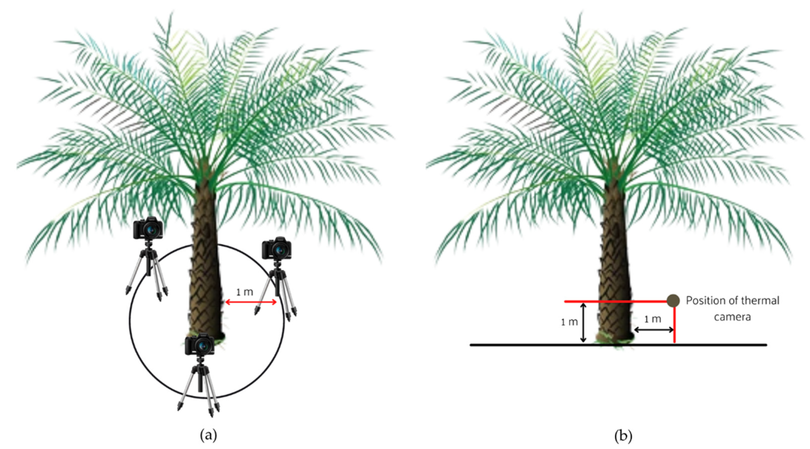
The FLIR T620 IR infrared thermal imaging camera (FLIR Systems, Inc., Wilsonville, OR, USA) was used for data acquisition. The trunk images of each tree section were randomly captured at three different angles. The age of the tree was 13 years old, having a height of more than 4 m. The thermal camera position was 1 m above the ground and 1m away from the tree. The image acquisition was carried out for trunk sections in two different sessions: morning and afternoon. For the morning session, the images were captured from 7.30 a.m. to 10 a.m. Meanwhile, the images in the afternoon session were captured from 4.30 p.m. to 7 p.m. This selection session was based on the sun’s heat energy gradually absorbed by crop plants during daylight hours. Moreover, as the ambient temperature rises throughout the day, these objects become less distinct from other warm objects that the camera’s sensor detects and highlights. An illustration diagram for the experimental setup of the trunk is shown in Figure 1.

To measure temperature accurately, the effects of several different radiation sources must therefore be offset, such as emissivity, reflected temperature, and other environmental parameters (atmospheric temperature, ecological humidity, and camera distance). The temperature of the object (T_obj) can be calculated from Equation (1). Different camera manufacturers use similar equations to perform temperature measurements [54]. In order to solve Equation (1), numerous parameter inputs are required by the camera, or software, to precisely estimate the temperature of the object.

$$T_{obj}={}^4\sqrt{\frac{W_{tot}-\left(1-{\epsilon }_{obj}\right) . {\tau }_{atm} . \sigma . {\left(T_{ref}\right)}^4-\left(1-{\tau }_{atm}\right) . \sigma . {\left(T_{atm}\right)}^4}{{\epsilon }_{obj} . {\tau }_{atm} . \sigma }}$$

(1)

where ε_obj refers to the object’s emissivity, T_ref refers to the reflected temperature, τ_atm refers to the transmittance of the atmosphere, and T_atm refers to the atmosphere’s temperature. Generally, the transmittance of the atmosphere is determined by the distance between the object and the camera and the relative humidity. This value is typically close to one. However, because the atmosphere’s emittance is close to zero (1 − τ_atm), this characteristic has a negligible effect on temperature measurements. On the other hand, the emissivity of the object and the reflected temperature have a significant impact on the temperature measurement and must be determined precisely.

2.1.1. Emissivity Measurement

Emissivity is the efficiency of an object to radiate heat. Provided that both the object and an ideal blackbody are at the same temperature, emissivity can be defined as the ratio of infrared energy emitted by the object, as compared to that emitted by an ideal blackbody and represented as a percent or a decimal. In this experimental study, the emissivity of the oil palm tree’s surface was estimated using an emissivity coating method [55]. If a part of the surface under study can be coated with a black paint with a known emissivity, the emissivity of the surface can be obtained by changing the emissivity value set on the device until the surface temperatures measured on the coated and uncoated surfaces are the same [56]. Several authors utilized a similar approach, except instead of black paint, black electrical tape was employed [57,58,59,60]. The configuration of the emissivity is then changed until the actual temperature is measured. The final configured emissivity is the emissivity of the object. As a result, at emissivity of 0.98, the oil palm tree’s temperature and the tape’s temperature recorded by the thermal camera were the same.

2.1.2. Reflected Apparent Temperature (RAT)

The reflected apparent temperature must be calibrated for accurate measurement. The object’s perceived temperature compensates for the radiation reflected from its surroundings into the camera. When the emissivity is low and the object temperature is significantly different from the reflected apparent temperature, it is even more crucial to set the reflected apparent temperature accurately. A crumpled and re-flattened sheet of aluminum foil is a frequently used substitute [55]. The reflector is positioned within the infrared camera’s field of view, and the reflector’s temperature is determined using an emissivity of one and a distance of zero. Finally, the test is repeated with the reflector’s temperature as the reflected temperature. The final reflected temperature is the resultant temperature value.

2.1.3. Atmospheric Temperature and Humidity

Additionally, the camera may take into account the effect of atmospheric temperature. The nature of the camera demonstrates that transmittance is dependent on the relative humidity present in the atmosphere. The temperature and humidity of the atmosphere were recorded every half hour using a TFA Dostmann Digital Thermo-Hygrometer (30.5002) (TFA-Dostmann.de., Wertheim-Reicholzheim, Germany).

2.1.4. The Distance between the Object and the Camera

Distance is a parameter that indicates the distance between an object and the front lens of the camera. In this research, the distance was fixed at 1 m. The camera was focused on the trunk of the oil palm tree at a height of 1 m above the ground, where the G. boninense fruiting bodies appear on the basal stem.

2.2. Data Pre-Processing

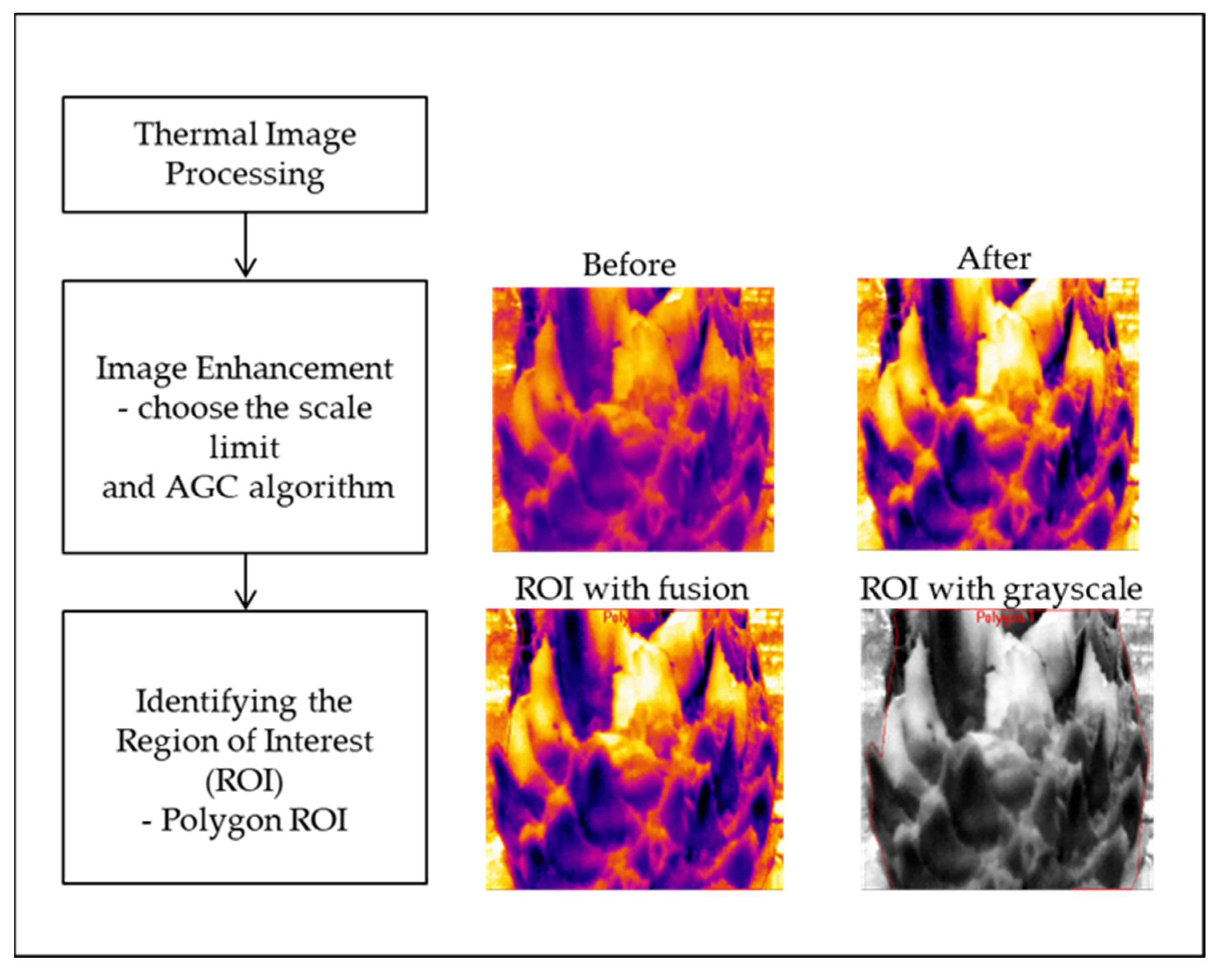
The temperature variation for each of the thermal images was analyzed using the camera manufacturer’s software, FLIR ResearchIR Max (FLIR Systems, Inc., Wilsonville, OR, USA). The two primary image processing steps involved in this study and the processing workflow are depicted in Figure 2.

2.2.1. Image Enhancement

Image enhancement seeks to improve the perceived utility of images for human viewers or help in processing other image-based techniques by computer. Two inputs for changing the image’s contrast are used in image enhancement, such as setting the limits for different scales and using automatic gain control (AGC) algorithms (these algorithms can improve image detail and contrast). This study used scale limits from image and plateau equalization (PE). Scale limits from image’s function is to look at the entire image to determine the min and max values for the scale; meanwhile, PE allows for excellent contrast in almost all scenes. Users can control the algorithm’s aggressiveness and choose how intense they want the image enhancements to be using a PE slider. In short, the outcome of image enhancement improves the image’s quality and can lead to better views of an image. Image differences before and after the image enhancement process can be seen in Figure 2.

2.2.2. Identifying the Region of Interest (ROI)

The first thing to consider is that the oil palm trunk area needs to be separated from its background. The process starts with recognizing different regions in the image that are likely to contain foreground objects. Defining the region of interest (ROI) is the first and primary step in thermography processing analysis. Current software uses various shapes, including a box, ellipse, line, bendable line, polygon, freehand, spot cursor, and measurement cursor for defining these regions. The ROI was represented in this study by a polygon. Polygons were selected due to the irregular trunk features of the oil palm tree. As a result, the ROI temperature was considered, as shown in Figure 2.

2.3. Feature Extraction—Thermal Image

Feature extraction is a technique for reducing the dimension of an image by efficiently representing remarkable regions as a compact feature vector. This method was carried out on the thermal images that had been processed. FLIR Tools in the FLIR ResearcherIR Max software environment was used to extract features from each thermal image. The following features were retrieved from the ROI of the thermal images that represent the oil palm trees denoted by $A={\left\{a_i\right\}}_{i=1}^N$ and are defined as below:

• Maximum temperature of oil palm trunk, (T_max) = max (A)
• Minimum temperature of oil palm trunk, (T_min) = min (A)
• Center temperature of oil palm trunk, (T_center) = center (A)
• Mean temperature of oil palm trunk, (T_mean) = $\frac{{{\displaystyle \sum }}_{i=1}^N{a}_i}{N}$
• Standard deviation temperature of oil palm trunk, (T_sd) = $\sqrt{\frac{1}{N}{\displaystyle \sum }_{i=1}^N{(a_i-T_{mean})}^2 }$

where N is total number of pixels and $a_i$ is pixel value at i.

Every feature was extracted from the three images taken at different angles and the values averaged. These averaged features were then used to analyze the characteristics of non-infected and infected trees using a statistical analysis of variance (ANOVA) using JMP Pro 16 (SAS Institute Inc., Cary, NC, USA).

2.4. Statistical Analysis

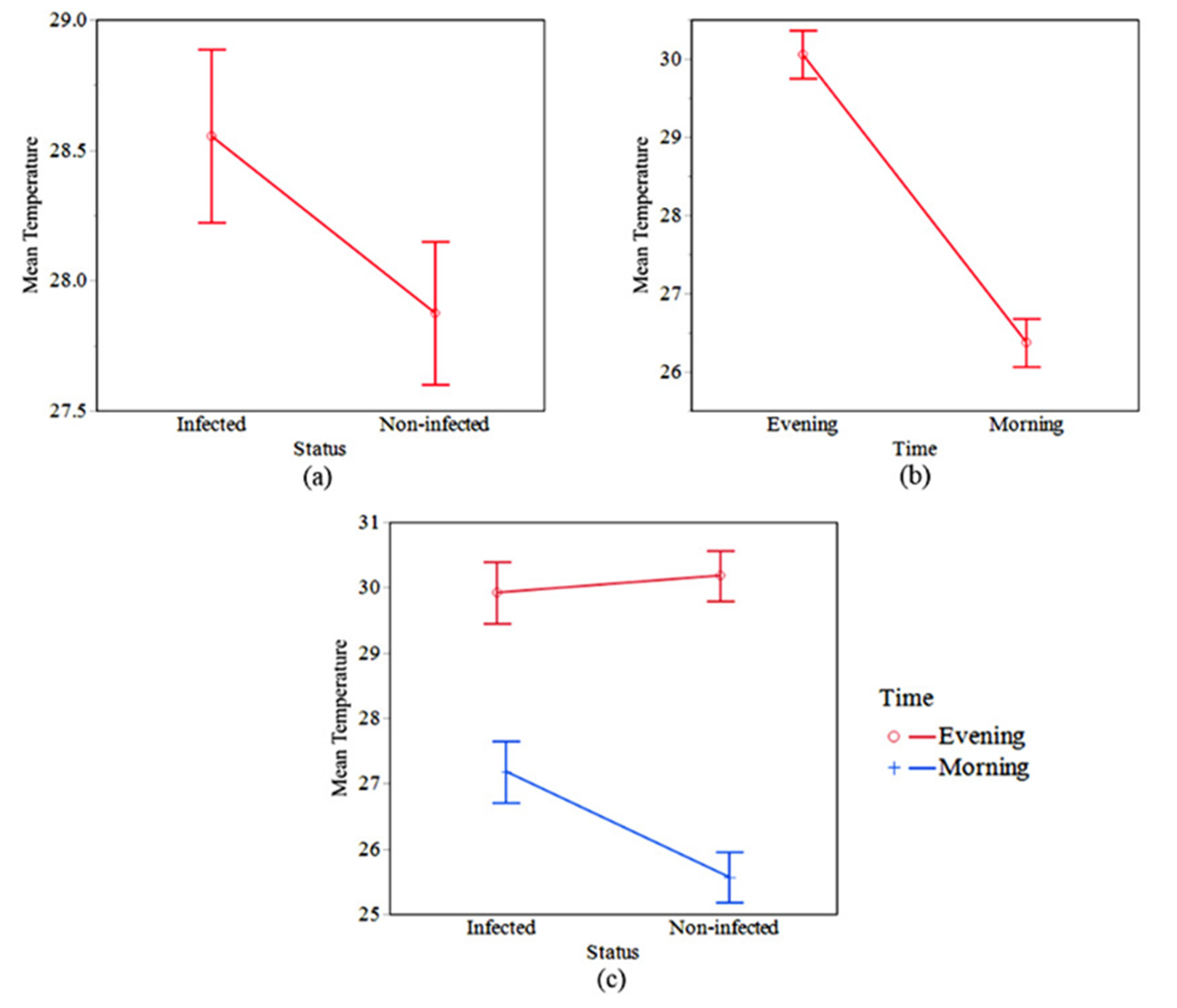
Since a series of comparisons were carried out in the present study, the variances were analyzed (through an ANOVA test) to see whether the means of dependent variables are different in the involved groups or not. In this study, an ANOVA test was conducted in the following order:

• to assess the temperature characteristic of the non-infected and infected trees during morning and evening sessions to see if there was a significant effect between non-infected and infected trees during morning and evening sessions;
• to evaluate the relationship between non-infected and infected trees and the feature temperature captured by the thermal camera.

2.5. Machine Learning Approach

Additionally, the machine learning approach can be utilized to categorize both large numbers of samples and small numbers of samples [22,61]. Classification is performed using the features retrieved from the thermal images as input. The extracted features act as the predictor while the oil palm status serves as a response. To differentiate between non-infected and BSR-infected trees, the classification was performed using the Waikato Environment for Knowledge Analysis (WEKA) version 3.8.5. We used cross-validation to evaluate the model’s performance due to the small sample size. WEKA’s K-fold cross-validation function divided the data into training and testing sets and carried out an independent assessment of the model’s accuracy. As a result, the model generated was acceptable and not restricted to a single collection of data. We performed ten iterations of cross-validation, randomly partitioning the original data into ten subsamples. Three ML techniques were employed, as follows:

(i) Naïve Bayes (NB). The NB algorithm is a probabilistic generative model based on the concept of conditional independence of predictor features, which means that the presence of one feature in a class is unrelated to any other feature [62]. NB’s conditional independence assumption enables the computation of the sample data’s class-conditional probabilities, which can be calculated directly from the training data rather than by assessing all feature possibilities [63].

(ii) Multilayer perceptron (MLP). MLP is an artificial neural network feed-forward model that charts input datasets to a set of appropriate outputs. An MLP is the result of multiple layers of nodes being connected [64]. Except for the input nodes, every node is a neuron (or processing element) with a nonlinear activation function. For training the network, MLP utilizes a supervised learning technique called backpropagation [65]. MLP is a modification of the standard linear perception and can distinguish non-linearly separable data.

(iii) Random forest (RF). RF is a classification algorithm that consists of a collection of stochastic decision trees. In RF, each tree is trained using a separate bootstrap sample from the original datasets, and each node contains a random feature from the original dataset [66]. The dataset is assigned using a majority vote obtained from an ensemble of trees constructed using the RF technique [67]. Additionally, it has high predictive accuracy, is resilient to noise, and is effective with an imbalanced dataset [68,69].

2.6. Imbalance Data Approach

Using ML, classifiers are developed with the goal of minimizing classification errors and increasing predicting accuracy. These classification methods make the basic assumption that the dataset under research comprises a well-balanced number of examples for each specific class of classifications. Therefore, the target classes’ prior probabilities are considered identical [70]. Classification algorithms have traditionally been motivated by improving the predicted accuracy of the generated classifiers.

Nonetheless, maximizing overall accuracy may not be the optimal strategy in the event of an unbalanced dataset. To maximize overall accuracy, a classifier concentrates on the majority class, which carries the maximum weight in the data. As a result, the classifier can achieve high accuracy on the majority class while doing poorly on the minority group due to the overall dataset extension. Our concern is with the minority class. Due to the small number of BSR-infected samples relative to non-infected samples, data imbalance was a challenge in this study. In machine learning, class imbalance can be addressed by either altering the underlying algorithm’s learning processes or modifying the dataset itself. The approach to solving this problem is a data-level approach. To increase the imbalance ratio, concerning data-level imbalance handling, the incidence of the two classes is algorithmically equated.

Data Sampling

The data-level approach is often referred to as the data sampling technique. It accomplishes this by artificially balancing the class instances in the dataset. Resampling corrects for imbalances by altering each class type instance, which frequently employs sampling techniques such as undersampling or oversampling, or a combination of the two [71]. Resampling techniques are more adaptable because they are not dependent on the classifier chosen [72].

(i) Undersampling is one of the simplest strategies to handle imbalanced data. The primary undersampling method arbitrarily eliminates majority class examples in order to balance the dataset [73]. The simplest yet most effective method is undersampling the majority class, most commonly implemented as random undersampling (RUS). In RUS, the majority of class instances are discarded at random until a more balanced distribution is attained [74]. Consider, for example, a dataset consisting of 100 majority class instances and 10 minority class instances. In RUS, by selecting 90 majority class instances at random to be removed, one might attempt to create a balanced class distribution. The resulting dataset will then have 20 instances: 10 (the original) minority class instances and 10 (randomly remaining) majority class instances.

(ii) Oversampling is another common sampling method employed in dealing with an imbalanced class problem. Numerous oversampling methods are available including random oversampling (ROS), focused oversampling, and synthetic sampling [75,76]. In ROS, minority class instances are copied and also repeated in the dataset until a more balanced distribution is attained. Therefore, if there are 100 majority class instances and two minority class instances, traditional oversampling would copy the two minority class instances 49 times. The resulting dataset will have 200 instances: the 100 majority class instances and 100 minority class instances (i.e., 50 of each of the two minority class instances). In focused oversampling, only those minority class values having samples that occur on the boundary between the majority and minority class values are resampled.

(iii) SMOTE is a method that generates synthetic samples to oversample the minority class [75]. SMOTE selects a representative of a minority class at random and then locates the nearest minority class neighbor. The synthetic instance is then constructed by randomly selecting one of the k-nearest neighbors, B, and linking A and B in space attributes to form a line segment. The synthetic samples are created by combining two selected samples, A and B, convexly [77]. Finally, new minority class instances are synthesized.

This study used resampling approaches such as RUS, ROS, and SMOTE. Resampling was performed using an open-source ML program, WEKA. Prior to classification, the resampling parameters were determined and are summarized in

Table 1. Summary of the parameters used for the imbalanced approach.

Technique	Parameter
RUS	distributionSpread = 1
ROS	biasToUniformClass = 1
	noReplacement = false
SMOTE	classValue = 0
	nearestNeighbors = 5
	percentage = 50

Random Undersampling (RUS), Random Oversampling (ROS), Synthetic Minority Oversampling (SMOTE).

.

We divided the dataset into 70% training and 30% test for testing purposes.

Table 2. A pre-processed dataset applying an imbalanced approach for non-infected and Basal Stem Rot (BSR)-infected trees.

	Training		Testing
	Non-Infected (Majority)	BSR-Infected (Minority)	Non-Infected (Majority)	BSR-Infected (Minority)
Single (without class imbalance approach)	38	25	17	12
RUS	25	25	12	12
ROS	31	31	14	14
SMOTE	38	38	17	17

illustrates the imbalanced technique used to pre-process the dataset for non-infected and BSR-infected trees.

2.7. Accuracy Assessment

Overall accuracy as an assessment metric will be biased because of the data imbalance problem since it mainly represents the majority class’s accuracy [54]. This analysis, therefore, presented the description of the confusion matrix as an alternative in terms of the success rate of the non-infected and BSR-infected trees, along with the receiver operating characteristic (ROC) curve region (AUC) and precision–recall curve (PRC). These metrics were used to evaluate different classifier and imbalanced approaches and measure their performance. The receiver operating characteristic (ROC) curve represents the degree or measure of separability, whereas the area under the curve (AUC) represents the degree or measure of separability. In AUC, the true positive rate (TPR), on the y-axis, is plotted against the false positive rate (FPR), on the x-axis [78]. The AUC is a good metric for classifier performance because it is decision-dependent, and the score is always confined between 0 and 1 [79]. No viable classifier has an AUC value less than 0.5 [80]. The higher the AUC value, the more capable the model is at discriminating between positive and negative classifications. The PRC is an alternative to the AUC. PRC is calculated and plotted as the precision (y-axis) versus recall (x-axis) for a single classifier at various thresholds [78]. In general, the greater the area under the PRC score, the better a classifier performs. In contrast to AUC, PRC does not take into account the number of true negative outcomes [81].

This study considered the AUC and PRC value of 0.50 as fail, 0.51–0.69 as poor, 0.70–0.79 as acceptable, 0.80–0.89 as excellent, and 0.90–1.00 as outstanding [82]. Meanwhile, this study classified the success rate of classifying the non-infected and BSR-infected trees as poor if it was less than 40.00 percent, moderate if it was 40.00–80.00 percent, and robust if it was more significant than 80.00 percent [83].

3. Results

3.1. Selection of the Time Session

In this study, the temperature characteristic of the non-infected and infected trees during morning and evening sessions was found. Figure 3 shows an example of the processed thermal image during the morning and evening session of a trunk section. The feature of the mean temperature was extracted from the thermal images. The results were compared to see if there was a significant effect between non-infected and infected trees during morning and evening sessions.

The two-way ANOVA was conducted to compare the main effects of status (non-infected and infected with BSR) and session (morning and evening) and their interaction effects on the mean temperature of the oil palm trees.

Table 3. Descriptive statistics for mean temperature extracted from the thermal images.

Status	Time	Mean	Std. Deviation	n
Non-infected	Morning	25.57	0.90	55
	Evening	30.18	1.44	55
Infected	Morning	27.18	1.91	37
	Evening	29.92	1.59	37

shows the descriptive statistics for mean temperature extracted from the thermal images.

Table 4. ANOVA summary table for mean temperature extracted from the thermal images.

Source	df	Mean Square	F	Sig.	Partial Eta Squared
Status	1	20.382	9.700	0.002	0.051
Session	1	598.529	284.851	0.000	0.613
Status * Time	1	39.073	18.596	0.000	0.094
Error	180	2.101
Total	183

*-Factor interactions, df-Degrees of Freedom, F-Variance Ratio, Sig.-Significant.

shows that the status and session effects were statistically significant at p < 0.005. The main effect for the status yielded an F ratio of F (1,180) = 9.70, p < 0.002, indicating a significant difference between non-infected oil palm trees and those infected with BSR. The main effect for the session yielded an F ratio of F (1,180) = 284.851, p < 0.001, indicating a significant difference between morning and evening sessions. The interaction effect was significant, F (1,180) = 18.596, p < 0.001. Therefore, this result shows that the data collection for the thermal image acquisition process can be carried out during morning and evening sessions for a trunk section. The relationship between feature temperature (T_mean) and the status of the oil palm trees is shown in Figure 4a; the relationship between feature temperature (T_mean) and the session captured in a thermal image in Figure 4b; and the interaction effect of feature temperature (T_mean) with the healthiness of oil palm and session in Figure 4c.

Figure 4a illustrates that the T_mean for BSR-infected trees is higher than for non-infected trees. Meanwhile, Figure 4b shows that the T_mean in the evening session is higher compared to the morning session. Furthermore, Figure 4c reveals that the T_mean for BSR-infected trees is higher than the non-infected trees in the morning session and contradicts the evening session result.

3.2. Feature Temperature Selection

The one-way analysis of variance (ANOVA) test evaluated the relations among non-infected and infected trees and the thermal camera’s feature temperature. The independent variables in the present study were non-infected and BSR-infected oil palm trees. On the other hand, the dependent variable consisted of T_mean, T_sd, T_center, T_max, and T_min extracted from the thermal image. These analyses helped determine whether the data on the healthiness oil palm trees differed significantly or not.

Table 5. The descriptive statistics for features extracted from the thermal images.

Feature	Status	Number of Samples(n)	Mean	Std. Deviation	Std. Error	95% Confidence Interval for Mean
						Lower Bound	Upper Bound
Tmean	Non-infected	55	25.566	0.902	0.122	25.322	25.810
	Infected	37	27.184	1.912	0.314	26.547	27.822
Tsd	Non-infected	55	0.422	0.121	0.016	0.389	0.455
	Infected	37	0.742	0.678	0.111	0.516	0.968
Tcenter	Non-infected	55	25.559	0.941	0.127	25.305	25.814
	Infected	37	27.208	2.131	0.350	26.498	27.918
Tmax	Non-infected	55	27.333	1.408	0.190	26.952	27.713
	Infected	37	30.842	4.976	0.818	29.183	32.501
Tmin	Non-infected	55	24.447	0.829	0.112	24.222	24.671
	Infected	37	25.567	0.993	0.163	25.235	25.898

shows the descriptive statistics for features extracted from the thermal images.

A summary of the results of the ANOVA test is presented in

Table 6. ANOVA results comparing the mean of T_mean, T_sd, T_center, T_max, and T_min between non-infected and BSR-infected oil palm trees.

Feature	p Value	Significance
Tmean	<0.0001	Yes
Tsd	<0.0001	Yes
Tcenter	<0.0001	Yes
Tmax	<0.0001	Yes
Tmin	0.0392	Yes

. The ANOVA result’s significance can be seen from all the feature temperatures, T_mean, T_sd, T_center, T_max, and T_min. It is then assumed that all the feature temperatures are suitable for further classification of the oil palm trees.

3.3. Classification Analysis of Feature Temperature

The features obtained from the thermal images were classified into non-infected and BSR-infected trees based on the imbalanced data approaches RUS, ROS, and SMOTE, and without an imbalanced data approach using several classification methods, namely, NB, MLP, and RF. The AUC, PRC, and success rate (%) of the non-infected trees and trees infected by G. boninense are shown in

Table 7. The area under the curve (AUC) of the NB, MLP, and RF classifiers according to temperature feature.

Feature	NB				MLP				RF
	Single	RUS	ROS	SMOTE	Single	RUS	ROS	SMOTE	Single	RUS	ROS	SMOTE
Tmean	0.787 c	0.722 c	0.797 c	0.801 d	0.806 d	0.766 c	0.785 c	0.823 d	0.665 b	0.710 c	0.800 d	0.734 c
Tsd	0.588 b	0.555 b	0.649 b	0.573 b	0.629 b	0.522 b	0.628 b	0.627 b	0.529 b	0.435 a	0.754 c	0.512 b
Tcenter	0.754 c	0.692 b	0.758 c	0.793 c	0.791 c	0.718 c	0.745 c	0.801 d	0.682 b	0.658 b	0.838 d	0.760
Tmax	0.765 c	0.638 b	0.762 c	0.796 c	0.833 d	0.752 c	0.797 c	0.846 d	0.881 d	0.798 c	0.921 e	0.899 d
Tmin	0.811 b	0.780 c	0.808 d	0.835 d	0.799 c	0.762 c	0.780 c	0.815 d	0.696 b	0.680 b	0.838 d	0.744 c
Tmean, Tsd	0.738 c	0.721 c	0.802 d	0.767 c	0.811 d	0.755 c	0.759 c	0.815 d	0.677 b	0.674 b	0.855 d	0.748 c
Tmax, Tmin	0.823 b	0.774 c	0.827 d	0.846 d	0.806 d	0.718 c	0.810 d	0.816 d	0.801 d	0.750 c	0.907 e	0.844 d
Tmean, Tsd, Tcenter, Tmax, Tmin	0.796 c	0.736 c	0.826 d	0.807 d	0.789 c	0.739 c	0.801 d	0.811 d	0.766 d	0.706 c	0.920 e	0.845 d

^a as fail, ^b as poor, ^c as acceptable, ^d as excellent, ^e as outstanding.

,

Table 8. The area precision–recall curve (PRC) of the NB, MLP, and RF classifiers according to temperature feature.

Feature	NB				MLP				RF
	Single	RUS	ROS	SMOTE	Single	RUS	ROS	SMOTE	Single	RUS	ROS	SMOTE
Tmean	0.784 c	0.697 b	0.760 c	0.771	0.777	0.721	0.737	0.791	0.648 b	0.659 b	0.780 c	0.728
Tsd	0.632 b	0.596 b	0.657 b	0.600 b	0.685 b	0.557 b	0.623 b	0.637 b	0.556 b	0.489 a	0.739 c	0.558 b
Tcenter	0.749 c	0.692 b	0.769 c	0.776 c	0.758 c	0.667 b	0.718 c	0.767 c	0.673 b	0.634 b	0.811 d	0.711 c
Tmax	0.782 c	0.634 b	0.736 c	0.783 c	0.814 d	0.724 c	0.764 c	0.827 d	0.864 d	0.758 c	0.902 e	0.877 d
Tmin	0.798 c	0.750 c	0.776 c	0.822 d	0.765 c	0.709 c	0.726 c	0.775 c	0.680 b	0.646 b	0.816 d	0.729 c
Tmean, Tsd	0.748 c	0.704 c	0.782 c	0.748 c	0.806 d	0.712 c	0.716 c	0.776 c	0.671 b	0.638 b	0.828 d	0.727 c
Tmax, Tmin	0.802 d	0.751 c	0.782 c	0.831 d	0.766 c	0.679 b	0.772 c	0.791 c	0.765 c	0.705 c	0.885 d	0.811 d
Tmean, Tsd, Tcenter, Tmax, Tmin	0.770 c	0.710 c	0.772 c	0.785 c	0.764 c	0.702 c	0.771 c	0.784 c	0.724 c	0.652 b	0.902 e	0.806 d

^a as fail, ^b as poor, ^c as acceptable, ^d as excellent, ^e as outstanding.

and

Table 9. The success rate (%) for non-infected (N) and BSR-infected (I) trees for feature temper-atures used.

Feature	IA	Classification Model
		NB		MLP		RF
		N	I	N	I	N	I
Tmean	Single	92.11c	44.00 b	84.21 c	72.00 b	73.68 b	36.00 a
	RUS	88.00 c	44.00 b	84.00 c	72.00 b	72.00 b	52.00 b
	ROS	90.32 c	48.39 b	77.42 b	74.19 b	70.97 b	90.32 c
	SMOTE	92.11 c	55.26 b	84.21 c	71.05 b	65.79 b	52.63 b
Tsd	Single	94.74 c	32.00 a	94.74 c	24.00 a	60.53 b	52.00 b
	RUS	92.00 c	24.00 a	88.00 c	24.00 a	44.00 b	48.00 b
	ROS	93.55 c	29.03 a	90.32c	35.48 a	70.97 b	80.65 c
	SMOTE	94.74 c	23.68 a	86.84 c	39.47 a	57.89 b	50.00 b
Tcenter	Single	92.11 c	48.00 b	89.47 c	56.00 b	73.68b	52.00 b
	RUS	92.00 c	48.00 b	80.00 c	56.00 b	72.00 b	52.00 b
	ROS	90.32 c	48.39 b	77.42 b	67.74 b	83.87 c	90.32 c
	SMOTE	92.11 c	55.26 b	86.84 c	65.79 b	76.32b	71.05 b
Tmax	Single	92.11 c	36.00 a	84.21 c	72.00 b	86.84 c	80.00 c
	RUS	92.00 c	36.00 a	84.00 c	60.00 b	80.00 c	72.00 c
	ROS	93.55 c	48.39 b	90.32c	74.19 b	87.10 c	100.00 c
	SMOTE	94.74 c	42.11b	81.58 c	76.32 b	84.21 c	81.58 c
Tmin	Single	94.74 c	63.63b	86.84 c	64.00 b	73.68 b	56.00 b
	RUS	84.00 c	64.00 b	76.00 b	64.00 b	64.00 b	60.00 b
	ROS	87.10 c	67.74 b	80.65 c	70.97 b	74.19 b	90.32 c
	SMOTE	89.47 c	65.79 b	84.21 c	65.79 b	71.05 b	65.79 b
Tmean, Tsd	Single	94.74 c	44.00 b	81.58 c	64.00 b	73.68 b	56.00 b
	RUS	92.00 c	36.00 a	84.00 c	68.00 b	72.00 b	72.00 b
	ROS	93.55 c	41.94 b	74.19 b	77.42 b	77.42 b	93.55 c
	SMOTE	94.74 c	42.11 b	84.21 c	71.05 b	76.32 b	68.42 b
Tmax, Tmin	Single	89.47 c	44.00 b	86.84 c	60.00 b	84.21 c	76.00 b
	RUS	88.00 a	44.00 b	76.00 b	64.00 b	76.00 b	80.00 c
	ROS	90.32 a	61.29 b	83.87 c	74.19 b	87.10 c	100.00 c
	SMOTE	89.47 a	57.89 b	84.21 c	63.16 b	84.21 c	81.58 c
Tmean, Tsd, Tcenter, Tmax, Tmin	Single	92.11 a	44.00 b	84.21 c	60.00 b	84.21 c	68.00 b
	RUS	88.00 a	40.00 a	80.00 c	64.00 b	76.00 b	68.00 b
	ROS	90.32 a	48.39 b	83.87 c	74.19 b	83.87 c	96.77 c
	SMOTE	92.11 a	52.63 b	84.21 c	65.79 b	84.21 c	81.58 c

^a as poor, ^b as moderate, ^c as robust.

, respectively.

The AUC and PRC results are relatively similar (Table 7 and Table 8). The best AUC and PRC (outstanding) results obtained from the T_max feature and the RF classifier and ROS approach were 0.921 and 0.902, respectively. Using the RF classifier and ROS approach, the T_max features improve AUC and PRC results compared to a single approach. The RUS approach yields the lowest AUC and PRC results on all features and classifiers.

Table 9 shows all feature success rates of three classifiers NB, MLP, and RF. NB delivers strong results when classifying non-infected trees, but its ability to classify BSR-infected trees is reduced compared to the other two classifiers. The T_max feature provides the best overall success rate for all three classifiers, while the RF classifier has the highest success rate for classifying non-infected and BSR-infected trees. Meanwhile, in terms of the imbalanced approach, using the RF classifier, the ROS approach has the highest success rate of 87.10% for non-infected trees and 100% for BSR-infected trees.

Table 10. ANOVA for the effect of features, imbalanced approaches, and classifiers on AUC and PRC across non-infected and BSR-infected trees.

Source	AUC				PRC
	DF	Sum of Squares	F Ratio	Prob > F	DF	Sum of Squares	F Ratio	Prob > F
Feature	7	0.451	139.611	<0.0001 *	7	0.254	95.663	<0.0001 *
Imbalance Approach	3	0.135	97.435	<0.0001 *	3	0.135	118.367	<0.0001 *
Classifier	2	0.003	3.394	0.0430 *	2	0.002	2.935	0.0641
Feature*Imbalance Approach	21	0.026	2.691	0.0031 *	21	0.018	2.279	0.0114 *
Feature*Classifier	14	0.068	10.496	<0.0001 *	14	0.056	10.610	<0.0001 *
Imbalance Approach*Classifier	6	0.067	24.031	<0.0001 *	6	0.080	34.975	<0.0001 *
Error	42	0.019			42	0.016
C. Total	95	0.769		<0.0001	95	0.561		<0.0001

*-The mean difference is significant at the 0.05 level.

shows the ANOVA model results for the effect of features, imbalanced approaches, classifiers, and two-way interaction (Feature*Imbalance Approach, Feature*Classifier, and Imbalance Approach*Classifier) on AUC and PRC across non-infected and BSR-infected trees. For the AUC and PRC response variable, two main factors (Feature and Imbalance Approach) and their two-way interaction are all statistically significant at the α = 0.05 level. One main factor, “Classifier”, was found to be not significant at this significance level for PRC.

The Tukey’s HSD test was performed since each of the main factors is statistically significant, indicating which levels of these factors result in significantly different performances than the other levels of that factor. The first part of

Table 11. Mean comparison of AUC and PRC obtained from Tukey’s HSD test according to features, imbalanced approaches, classifiers, and classifier and imbalance approach interaction.

Feature
AUC	Mean	PRC	Mean
Tmax, Tmin	0.810 a	Tmax	0.789 a
Tmax	0.807 a	Tmax, Tmin	0.778 ab
Tmean, Tsd, Tcenter, Tmax, Tmin	0.795 ab	Tmean, Tsd, Tcenter, Tmax, Tmin	0.762 bc
Tmin	0.779 bc	Tmin	0.749 cd
Tmean	0.766 cd	Tmean, Tsd	0.738 cd
Tmean, Tsd	0.760 cd	Tmean	0.737 cd
Tcenter	0.749 d	Tcenter	0.727 d
Tsd	0.583 e	Tsd	0.611 e
Imbalance Approach
AUC	Mean	PRC	Mean
ROS	0.799 a	ROS	0.772 a
SMOTE	0.777 b	SMOTE	0.759 a
Single	0.751 c	Single	0.741 b
RUS	0.698 d	RUS	0.674 c
Classifier
AUC	Mean	PRC	Mean
MLP	0.764 a	NB	0.742 a
NB	0.754 ab	MLP	0.737 a
RF	0.751 b	RF	0.730 a
Imbalance Approach*Classifier
AUC	Mean	PRC	Mean
ROS-RF	0.854 a	ROS-RF	0.833 a
SMOTE-MLP	0.794 b	SMOTE-MLP	0.769 b
Single-MLP	0.783 b	Single-MLP	0.767 b
ROS-NB	0.779 b	SMOTE-NB	0.765 b
SMOTE-NB	0.777 b	Single-NB	0.758 bc
ROS-MLP	0.763 b	ROS-NB	0.754 bc
SMOTE-RF	0.761 b	SMOTE-RF	0.743 bc
Single-NB	0.758 b	ROS-MLP	0.728 cd
RUS-MLP	0.717 c	Single-RF	0.698 de
Single-RF	0.712 cd	RUS-NB	0.692 e

* Means with different letters in the same column according to group types are significantly different at p < 0.05.

provides HSD test results for the main factor feature. This factor has eight levels (the eight different features of temperature used for classification), each of which is assigned to a group (indicated by a letter) based on its average performance (across all the other factors). All the response variables’ results show a relatively consistent result for AUC and PRC. The combination feature T_max, T_min outperforms all other features in the AUC, and T_max outperforms all other features in the PRC. The Tukey’s HSD test demonstrated the combination of feature T_max, T_min was not statistically different from the T_max feature and combination T_mean, T_sd, T_center, T_max, T_min, but it significantly differed from the other temperature feature in AUC. Meanwhile, in PRC, the T_max feature was not statistically different from the combination feature T_max, T_min, but it significantly differed from the other temperature features. However, the T_sd feature is demonstrated to be lower than the statistically significant margin of all other temperature features.

The four imbalance approaches’ main factor levels perform significantly differently, with the ROS approach outperforming all three other approaches in AUC and PRC. Meanwhile, the RUS approach is lower than the statistically significant margin of all other imbalance approaches.

In AUC, MLP was not statistically different from NB, but it significantly differed from the RF. There is no statistical difference for the main factor of the three classifiers present in PRC.

Table 11 also shows the mean AUC and PRC values for the imbalance approach and classifier interaction. ROS-RF had a higher mean value and significantly differed from other interactions for the imbalance approach and classifier. The bottom performer was RUS-RF for AUC and PRC results.

4. Discussion

4.1. Selection of the Time Session

A tree trunk’s temperature influences a tree’s physiological processes and the microclimate for insects, parasites, fungi, and other organisms. Trunk temperatures may be significant in the translocation of water and photosynthates. The thermal properties of a tree (absorptivity, specific heat, and conductivity) combined with geometrical factors govern heat energy distribution [84].

In plants, water is absorbed from the soil into the plant’s roots, then up through the xylem into the leaves to be used differently for the plant’s continuance and help the plant maintain its temperature. Transpiration has two important functions: cooling and maintaining the plant temperature and transporting nutrients to the leaves for photosynthesis [85]. Transpiration is an evaporative cooling system that brings down plants’ temperature, but it must be accurately regulated since it leads to water loss. Most of the water in plants is lost through transpiration when the water is warmed by the sun and evaporated into vapor through thousands of stomata, mostly on the leaf surface’s underside.

The surface temperature of the trunk will respond to environmental factors almost instantaneously. In comparison, at a significant depth in the trunk, the temperature may take time to follow the surface. In a BSR-infected oil palm tree, restricted water uptake due to the damaged basal tissue causes the transpiration rate to become low. As the plant cannot cool down its temperature, it causes the infected tree’s temperature to be higher than a non-infected tree [86].

Due to the contradictory finding that the temperature of BSR-infected trees is lower in the evening than that of non-infected trees, this phenomenon can be expanded by referring to [35] who observed peanut leaf spots. As dead or severely damaged leaf tissue has a lower thermal capacity than normal tissue, it can be heated more easily and exhibits a greater radiance. Dead leaf tissue, on the other hand, can be cooled more quickly than healthy tissue. This fact explains the diseased plant’s increased radiance in the afternoon, corresponding to the decrease in air temperature. Two damaged trees of similar species, even when they have the same pathology, can generate different thermal patterns because the availability of water to which the tree is subject to differs and varies with the temperature gradient along the trunk/tree [87]. The temperature pattern, which allows identifying functional or dysfunctional tissues, is unique for each tree.

As mentioned above, the non-infected tree and infected tree characteristics have significant differences in the morning and evening. It is shown that oil palms’ health status can be determined when thermal images are taken in the morning (7.30 a.m. to 10 a.m.) and in the evening (4.30 p.m. to 7 p.m.). However, we used only morning session data in this study because thermal cameras are typically more effective in the early morning than in the afternoon [88,89].

4.2. Effect of Temperature Feature

One of the objectives of this study was to determine the potential of the temperature feature for classifying BSR disease in oil palm plants. Numerous studies have demonstrated the efficacy of thermal imaging in detecting temperature variations caused by water stress in plants. When transpiration happens and water is drained from the plants, the temperature of the plants decreases. Transpiration is a thermodynamic process that is endo-energetic. When plants are water-stressed in the soil, they frequently respond by decreasing their stomata conductance, decreasing transpiration. In an oil palm tree infected with BSR, the reduced water intake caused by the damaged basal tissue results in a poor transpiration rate. The disruption of water and nutrient transport caused by trunk damage has a detrimental effect on numerous elements of plant physiology, most notably photosynthetic potential [90]. The initial symptoms of BSR in oil palm are visible in the leaves, and this occurs after at least 50% of the cross-sectional area of the stem base has been injured. The rot impedes nutrient and water availability to the aerial regions, resulting in symptoms similar to nutritional imbalance and water stress [91].

Ref. [92] conducted a study of the existing literature on the application of infrared thermography to tree health assessment. While the majority of studies focused on pest detection and water stress detection, a small number of them examined wood degradation and cavity formation. Ref. [93] proposed detecting structural tree defects by analyzing the surface temperature of the tree trunk and discovered that the temperature of the tree bark surface varied significantly from the temperature of decayed wood areas. Due to the difference in moisture content between tree trunks with and without cavities, the emissivity varies, resulting in a difference in temperature observed by a thermal camera even though the temperature is the same [87]. The change in temperature patterns is an indication of an unhealthy state and enables scientific detection of tree cavities early. Trees have varying cooling impacts on the surface temperature depending on their kind and degree of decay. As a result, thermal imaging of the trunk temperature can assist in determining the temperature difference between healthy and unhealthy trees.

Our study discovered an outstanding outcome: classification of oil palm trees that are non-infected and BSR-infected can be successfully carried out using temperature parameters retrieved from thermal data. For all three classifiers, the T_max feature followed by the combination of T_max and T_min is more successful at accurately classifying non-infected and G. boninense-infected oil palm plants.

4.3. Effects of Data Imbalance on Classification

Classification, being a supervised learning process, depends mainly on the training data. The level of training plays a major role in the resultant accuracy of the classifier. The imbalanced nature of the datasets is a huge downside in this scenario. Due to the minimal occurrence of the minor classes, the classifier is insufficiently trained and hence provides inaccurate predictions. In the case of multiclass classifiers, such imbalance results in low representation of entries and, eventually, these entries tend to be totally ignored [94]. Most classifiers tend to implicitly consider their data as balanced; hence, standard classifiers are biased towards the majority.

Countering imbalance in data tends to be one of the major areas of research where real-time classification is concerned. Classifiers operating on data have a basic assumption that the data are balanced. Hence, the weight provided to each of the samples is equal [95]. However, in imbalanced data, this mode of operation makes the classifier biased towards the majority classes. Provided with a sufficiently high level of imbalance, the minority classes can even be ignored during the rule-building process. Data balancing techniques have been proposed to handle this scenario [96,97]. Data handling can be carried out by modifying the existing algorithms to increase weightage of the minority classes [78], increasing their contribution levels or sampling [98,99,100].

This study deals with the RUS, ROS, and SMOTE imbalanced approaches to counter the imbalance problem. This is not an exhaustive list of techniques but rather a starting point to handle imbalanced data. It was observed from this study that the ROS approach performs better compared to the single (without class imbalance) approach. It has better success classifying non-infected and BSR-infected oil palm trees. However, there is no best approach or model suited for all problems, and it is strongly recommended to try different techniques and models to evaluate what works best.

4.4. Effects of Classifiers on the Model Performance

All three ML models used in this study have nearly similar performance in classifying the oil palm trees based on the AUC, PRC, and success rate of non-infected trees and trees infected by G. boninense. We need a thorough understanding of these methods’ output to make maximum use of each classification system.

When adopting an algorithm, there are two factors to consider: (1) performance: when selecting a classification or regression algorithm, the total output of the algorithm is a significant determinant. (2) Robustness: when evaluating performance, it is crucial to consider the application’s robustness rather than the fitting’s consistency [101]. We eliminate the possibility of excessive generalization in this circumstance. This can be mitigated by limiting the number of models that an algorithm can recommend. Both MLP and RF can be utilized in this manner, each with its own set of advantages and limitations. The number of hidden neurons and layers in an MLP model has a significant impact on the model’s complexity and the amount of regularization employed while optimizing the weights. We can adjust the size and number of trees and the size and depth of individual trees to address the issue. Additionally, each of these techniques is capable of coping with ambiguity and overfitting. In contrast to NB, when classifying a new instance, the algorithm calculates the conditional probability of each class value. It selects the class with the highest probability as the anticipated class [102]. The method estimates all required probability values using the training data. To maintain tractability during computation, the approach makes the naïve assumption that all attribute values are conditionally independent of the class value.

In reality, all these three methods help with various characteristics of applications. No single algorithm can be beneficial in every case, according to ML. As a result, no single approach consistently outperforms others, and the outcomes of an algorithm will vary significantly depending on the application and dataset size. Thus, one can compare the outputs of multiple learning algorithms for a given task to determine the optimal algorithm. It is also good to put together ensembles of many models created using different methods to combine their strengths and minimize their flaws.

5. Conclusions

In this study, the feature properties of oil palm trees were extracted from thermal data and divided into two status levels: non-infected and infected by G. boninense. Eight (8) temperature features were used, namely, T_mean, T_sd, T_center, T_max, T_min, a combination of T_mean, T_sd, T_max, T_min, and T_mean, T_sd, T_center, T_max, T_min. Single, RUS, ROS, and SMOTE approaches were used with three classifier models NB, MLP, and RF.

In a comparison of performance, the AUC and PRC results for all feature temperatures (except T_sd) increased when using all three classifiers with the ROS approach instead of the single approach. In terms of model performance in the ROS approach, given any temperature features, the RF model had an AUC ranging from 0.754 to 0.921 compared to 0.649 to 0.827 for the NB model and 0.628 to 0.810 for the MLP model. Comparison between the RF, NB, and MLP models for the PRC gave a range of 0.739–0.902, 0.657–0.782, and 0.623–0.772, respectively.

Regarding the temperature features, specific features such as T_max stand out more than others. Using the most significant variable, T_max, the RF model had an AUC of 0.921 compared to 0.797 for the MLP model and 0.762 for the NB model. For PRC, a comparison of the RF model, the MLP model, and the NB model yielded values of 0.902, 0.764, and 0.736.

In conclusion, by using only the T_max feature, RF can predict BSR disease with a relatively outstanding accuracy compared to the MLP and NB which had an acceptable accuracy. The significant benefit derived from this study is the potential of using thermal data and the imbalanced data approach to classify oil palm trees infected by G. boninense using ML techniques. In the future, studies with samples of different severity levels will be used to analyze temperature features and identify oil palm trees that have been infected with BSR disease.

References

1. Chang, F.K. Palm Oil: Malaysian Economic Interests and Foreign Relations—Foreign Policy Research Institute. Available online: https://www.fpri.org/article/2021/04/palm-oil-malaysian-economic-interests-and-foreign-relations/ (accessed on 6 August 2021).
2. Department of Statistics Malaysia Selected Agricultural Indicators, Malaysia. 2020. Available online: https://www.dosm.gov.my/v1/index.php?r=column/cthemeByCat&cat=72&bul_id=RXVKUVJ5TitHM0cwYWxlOHcxU3dKdz09&menu_id=Z0VTZGU1UHBUT1VJMFlpaXRRR0xpdz09 (accessed on 6 August 2021).
3. Kondalamahanty, A. INTERVIEW: Malaysia 2021 Palm Oil Output Seen up on Better Weather, Yield: MPOB Chief. Available online: https://www.spglobal.com/platts/en/market-insights/latest-news/agriculture/060821-interview-malaysia-2021-palm-oil-output-seen-up-on-better-weather-yield-mpob-chief (accessed on 29 October 2021).
4. Chung, G. Management of Ganoderma diseases in oil palm plantations. Planter 2011, 87, 325–339. [Google Scholar]
5. Siddiqui, Y.; Surendran, A.; Paterson, R.R.M.; Ali, A.; Ahmad, K. Current strategies and perspectives in detection and control of basal stem rot of oil palm. Saudi J. Biol. Sci. 2021, 28, 2840–2849. [Google Scholar] [CrossRef]
6. Durand-Gasselin, T.; Asmady, H.; Flori, A.; Jacquemard, J.C.; Hayun, Z.; Breton, F.; de Franqueville, H. Possible sources of genetic resistance in oil palm (Elaeis guineensis Jacq.) to basal stem rot caused by Ganoderma boninense—prospects for future breeding. Mycopathologia 2005, 159, 93–100. [Google Scholar] [CrossRef]
7. Sahebi, M.; Hanafi, M.M.; Wong, M.-Y.; Idris, A.S.; Azizi, P.; Jahromi, M.F.; Shokryazdan, P.; Abiri, R.; Mohidin, H. Towards immunity of oil palm against Ganoderma fungus infection. Acta Physiol. Plant. 2015, 37, 1–16. [Google Scholar] [CrossRef]
8. Rees, R.W.; Flood, J.; Hasan, Y.; Wills, M.A.; Cooper, R.M. Ganoderma boninense basidiospores in oil palm plantations: Evaluation of their possible role in stem rots of Elaeis guineensis. Plant Pathol. 2012, 61, 567–578. [Google Scholar] [CrossRef] [Green Version]
9. Maluin, F.N.; Hussein, M.Z.; Idris, A.S. An Overview of the Oil Palm Industry: Challenges and Some Emerging Opportunities for Nanotechnology Development. Agronomy 2020, 10, 356. [Google Scholar] [CrossRef] [Green Version]
10. Hushiarian, R.; Yusof, N.A.; Dutse, S.W. Detection and control of Ganoderma boninense: Strategies and perspectives. Springerplus 2013, 2, 555. [Google Scholar] [CrossRef] [PubMed] [Green Version]
11. Priwiratama, H.; Susanto, A. Utilization of Fungi for the Biological Control of Insect Pests and Ganoderma Disease in the Indonesian Oil Palm Industry. J. Agric. Sci. Technol. 2014, 4, 103–111. [Google Scholar]
12. Khaled, A.Y.; Abd Aziz, S.; Bejo, S.K.; Nawi, N.M.; Seman, I.A.; Onwude, D.I. Early detection of diseases in plant tissue using spectroscopy–applications and limitations. Appl. Spectrosc. Rev. 2018, 53, 36–64. [Google Scholar] [CrossRef]
13. Khosrokhani, M.; Bejo, S.K.; Pradhan, B. Geospatial technologies for detection and monitoring of Ganoderma basal stem rot infection in oil palm plantations: A review on sensors and techniques. Geocarto Int. 2018, 33, 260–276. [Google Scholar] [CrossRef]
14. Izzuddin, M.A.; Hamzah, A.; Nisfariza, M.N.; Idris, A.S. Analysis of Multispectral Imagery From Unmanned Aerial Vehicle (UAV) using Object-Based Image Analysis for Detection of Ganoderma Disease in Oil Palm. J. Oil Palm Res. 2020, 32, 497–508. [Google Scholar] [CrossRef]
15. Izzuddin, M.A.; Ezzati, B.; Nisfariza, M.N.; Idris, A.S.; Alias, S.A. Analysis of Red, Green, Blue (RGB) and Near Infrared (NIR) Images from Unmanned Aerial Vehicle (UAV) for Detection of Ganoderma Disease in Oil Palm. Oil Palm Bull. 2019, 79, 9–15. [Google Scholar]
16. Izzuddin, M.A.; Nisfariza, M.N.; Ezzati, B.; Idris, A.S.; Steven, M.; Byod, D. Analysis of Airborne Hyperspectral Image using Vegetation Indices, Red Edge Position and Continuum Removal for Detection of Ganoderma Disease in Oil Palm. J. Oil Palm Res. 2018, 30, 416–428. [Google Scholar] [CrossRef]
17. Santoso, H. Performa Random Forest Group untuk Klasifikasi Penyakit Busuk Pangkal Batang yang Disebabkan oleh Ganoderma boninense pada Perkebunan Kelapa Sawit. J. Penelit. Kelapa Sawit 2020, 28, 133–146. [Google Scholar] [CrossRef]
18. Santoso, H.; Tani, H.; Wang, X.; Prasetyo, A.E.; Sonobe, R. Classifying The Severity of Basal Stem Rot Disease in Oil Palm Plantations Using Worldview-3 Imagery and Machine Learning Algorithms. Int. J. Remote Sens. 2019, 40, 7624–7646. [Google Scholar] [CrossRef]
19. Azmi, A.N.N.; Bejo, S.K.; Jahari, M.; Muharam, F.M.; Yule, I.; Husin, N.A. Early Detection of Ganoderma boninense in Oil Palm Seedlings Using Support Vector Machines. Remote Sens. 2020, 12, 3920. [Google Scholar] [CrossRef]
20. Bejo, S.K.; Jaleni, M.; Husin, M.E.; Khosrokhani, M.; Muharam, F.M.; Seman, I.A.; Anuar, M.I. Basal Stem Rot (BSR) Detection Using Textural Analysis of Unmanned Aerial Vehicle (UAV) Image. Proc. eProc. Chem. 2018, 3, 40–45. [Google Scholar]
21. Husin, N.A.; Bejo, S.K.; Abdullah, A.F.; Kassim, M.S.M.; Ahmad, D.; Azmi, A.N.N. Application of Ground-Based LiDAR for Analysing Oil Palm Canopy Properties on the Occurrence of Basal Stem Rot (BSR) Disease. Sci. Rep. 2020, 10, 6464. [Google Scholar] [CrossRef] [Green Version]
22. Husin, N.A.; Bejo, S.K.; Abdullah, A.F.; Kassim, M.S.M.; Ahmad, D.; Aziz, M.H.A. Classification of Basal Stem Rot Disease in Oil Palm Plantations Using Terrestrial Laser Scanning Data and Machine Learning. Agronomy 2020, 10, 1624. [Google Scholar] [CrossRef]
23. Husin, N.A.; Bejo, S.K.; Abdullah, A.F.; Kassim, M.S.M.; Ahmad, D. Analysis of Changes in Oil Palm Canopy Architecture From Basal Stem Rot Using Terrestrial Laser Scanner. Plant Dis. 2019, 103, 3218–3225. [Google Scholar] [CrossRef] [Green Version]
24. Toh, C.M.; Izzuddin, M.A.; Ewe, H.T.; Idris, A.S. Analysis of Oil Palms with Basal Stem Rot Disease with L Band SAR Data. Int. Geosci. Remote Sens. Symp. 2019, 4900–4903. [Google Scholar] [CrossRef]
25. Hashim, I.C.; Shariff, A.R.M.; Bejo, S.K.; Muharam, F.M.; Ahmad, K. Machine-Learning Approach Using SAR Data for the Classification of Oil Palm Trees That Are Non-Infected and Infected with the Basal Stem Rot Disease. Agronomy 2021, 11, 532. [Google Scholar] [CrossRef]
26. Kresnawaty, I.; Mulyatni, A.S.; Eris, D.D.; Prakoso, H.T.; Tri-Panji; Triyana, K.; Widiastuti, H. Electronic nose for early detection of basal stem rot caused by Ganoderma in oil palm. In Proceedings of the IOP Conference Series: Earth and Environmental Science; Institute of Physics Publishing: Bristol, UK, 2020; Volume 468. [Google Scholar]
27. Abdullah, A.H.; Adorn, A.H.; Shakaff, A.Y.M.; Ahmad, M.N.; Saad, M.A.; Tan, E.S.; Fikri, N.A.; Markom, M.A.; Zakaria, A. Electronic Nose System for Ganoderma detection. Sens. Lett. 2011, 9, 353–358. [Google Scholar] [CrossRef]
28. Mazliham, M.S.; Loonis, P.; Idris, A.S. Interpretation of Sound Tomography Image for the Recognition of Ganoderma Infection Level in Oil Palm. In Trends in Intelligent Systems and Computer Engineering; Springer: Boston, MA, USA, 2008; Volume 6, pp. 409–426. [Google Scholar]
29. Hamidon, N.A.; Mukhlisin, M. View of A Review of Application of Computed Tomography on Early Detection of Basal Stem Rot Disease. J. Teknol. 2014, 70, 45–47. [Google Scholar]
30. Yusoff, M.; Khalid, A.; Seman, I.A. Identification of Basal Stem Rot Disease In Local Palm Oil by Microfocus XRF. J. Nucl. Relat. Technol. 2009, 6, 282–287. [Google Scholar]
31. Harrap, M.J.M.; De Ibarra, N.H.; Whitney, H.M.; Rands, S.A. Reporting of thermography parameters in biology: A systematic review of thermal imaging literature. R. Soc. Open Sci. 2018, 5, 1–20. [Google Scholar] [CrossRef] [Green Version]
32. Xu, H.; Zhu, S.; Ying, Y.; Jiang, H. Early detection of plant disease using infrared thermal imaging. In Proceedings of the SPIE 6381, Optics for Natural Resources, Agriculture, and Foods; International Society for Optics and Photonics: Boston, MA, USA, 2006; Volume 6381, p. 638110. [Google Scholar]
33. Oerke, E.-C.; Fröhling, P.; Steiner, U. Thermographic assessment of scab disease on apple leaves. Precis. Agric. 2011, 12, 699–715. [Google Scholar] [CrossRef]
34. Jafari, M.; Minaei, S.; Safaie, N. Detection of pre-symptomatic rose powdery-mildew and gray-mold diseases based on thermal vision. Infrared Phys. Technol. 2017, 85, 170–183. [Google Scholar] [CrossRef]
35. Omran, E.S.E. Early sensing of peanut leaf spot using spectroscopy and thermal imaging. Arch. Agron. Soil Sci. 2017, 63, 883–896. [Google Scholar] [CrossRef]
36. Bejo, S.K.; Abdol Lajis, G.; Abd Aziz, S.; Seman, I.A.; Ahamed, T. Detecting Basal Stem Rot (BSR) Disease at Oil Palm Tree Using Thermal Imaging Technique. In Proceedings of the 14th International Conference on Precision Agriculture, Montreal, QC, Canada, 24–27 June 2018; pp. 1–8. [Google Scholar]
37. Johari, S.N.Á.M.; Bejo, S.K.; Lajis, G.A.; DaimDai, L.D.J.; Keat, N.B.; Ci, Y.Y.; Ithnin, N. Detecting BSR-infected Oil Palm Seedlings using Thermal Imaging Technique. Basrah J. Agric. Sci. 2021, 34, 73–80. [Google Scholar] [CrossRef]
38. Chang, C.-W.; Lee, H.-W.; Liu, C.-H. A Review of Artificial Intelligence Algorithms Used for Smart Machine Tools. Inventions 2018, 3, 41. [Google Scholar] [CrossRef] [Green Version]
39. Ayaz Mirani, A.; Suleman Memon, M.; Chohan, R.; Ali Wagan, A.; Qabulio, M. Machine Learning in Agriculture: A Review. LUME 2021, 10, 5. [Google Scholar]
40. More, S.; Singla, J. Machine learning techniques with IoT in agriculture. Int. J. Adv. Trends Comput. Sci. Eng. 2019, 8, 742–747. [Google Scholar] [CrossRef]
41. Liakos, K.G.; Busato, P.; Moshou, D.; Pearson, S.; Bochtis, D. Machine learning in agriculture: A review. Sensors 2018, 18, 2674. [Google Scholar] [CrossRef] [PubMed] [Green Version]
42. Abdi, A.M. Land cover and land use classification performance of machine learning algorithms in a boreal landscape using Sentinel-2 data. GIScience Remote Sens. 2020, 57, 1–20. [Google Scholar] [CrossRef] [Green Version]
43. Jamali, A. Land use land cover mapping using advanced machine learning classifiers: A case study of Shiraz city, Iran. Earth Sci. Inform. 2020, 13, 1015–1030. [Google Scholar] [CrossRef]
44. Pan, L.; Gu, L.; Ren, R.; Yang, S. Land cover classification based on machine learning using UAV multi-spectral images. In Proceedings of the Earth Observing Systems XXV; International Society for Optics and Photonics: Boston, MA, USA, 2020; Volume 11501, p. 115011F. [Google Scholar]
45. Liu, Z.; Peng, C.; Work, T.; Candau, J.N.; Desrochers, A.; Kneeshaw, D. Application of machine-learning methods in forest ecology: Recent progress and future challenges. Environ. Rev. 2018, 26, 339–350. [Google Scholar] [CrossRef] [Green Version]
46. Lee, J.; Im, J.; Kim, K.; Quackenbush, L.J. Machine Learning Approaches for Estimating Forest Stand Height Using Plot-Based Observations and Airborne LiDAR Data. Forests 2018, 9, 268. [Google Scholar] [CrossRef] [Green Version]
47. Li, M.; Im, J.; Beier, C. Machine learning approaches for forest classification and change analysis using multi-temporal Landsat TM images over Huntington Wildlife Forest. GIScience Remote Sens. 2013, 50, 361–384. [Google Scholar] [CrossRef]
48. Sharma, A.; Jain, A.; Gupta, P.; Chowdary, V. Machine Learning Applications for Precision Agriculture: A Comprehensive Review. IEEE Access 2021, 9, 4843–4873. [Google Scholar] [CrossRef]
49. Khaled, A.Y.; Abd Aziz, S.; Bejo, S.K.; Nawi, N.M.; Abu Seman, I. Spectral features selection and classification of oil palm leaves infected by Basal stem rot (BSR) disease using dielectric spectroscopy. Comput. Electron. Agric. 2018, 144, 297–309. [Google Scholar] [CrossRef]
50. Santoso, H.; Tani, H.; Wang, X. Random Forest classification model of basal stem rot disease caused by Ganoderma boninense in oil palm plantations. Int. J. Remote Sens. 2017, 38, 4683–4699. [Google Scholar] [CrossRef]
51. Thabtah, F.; Hammoud, S.; Kamalov, F.; Gonsalves, A. Data imbalance in classification: Experimental evaluation. Inf. Sci. 2020, 513, 429–441. [Google Scholar] [CrossRef]
52. Chemchem, A.; Alin, F.; Krajecki, M. Combining SMOTE sampling and machine learning for forecasting wheat yields in France. In Proceedings of the Proceedings—IEEE 2nd International Conference on Artificial Intelligence and Knowledge Engineering, AIKE 2019, Sardinia, Italy, 3–5 June 2019; pp. 9–14. [Google Scholar]
53. Ma, H.; Huang, W.; Jing, Y.; Yang, C.; Han, L.; Dong, Y.; Ye, H.; Shi, Y.; Zheng, Q.; Liu, L.; et al. Integrating growth and environmental parameters to discriminate powdery mildew and aphid ofwinter wheat using bi-temporal Landsat-8 imagery. Remote Sens. 2019, 11, 846. [Google Scholar] [CrossRef] [Green Version]
54. Frank, E. Liebmann Infrared Target Temperature Correction System and Method 2010. U.S. Patent 7,661,876, 16 February 2010. [Google Scholar]
55. Usamentiaga, R.; Venegas, P.; Guerediaga, J.; Vega, L.; Molleda, J.; Bulnes, F.G. Infrared Thermography for Temperature Measurement and Non-Destructive Testing. Sensors 2014, 14, 12305–12348. [Google Scholar] [CrossRef] [Green Version]
56. Buchlin, J.M. Convective Heat Transfer and Infrared Thermography (IRTH). J. Appl. Fluid. Mech. 2010, 3, 55–62. [Google Scholar]
57. Bazilian, M.D.; Kamalanathan, H.; Prasad, D.K. Thermographic analysis of a building integrated photovoltaic system. Renew. Energy 2002, 26, 449–461. [Google Scholar] [CrossRef]
58. Avdelidis, N.; Moropoulou, A. Emissivity considerations in building thermography. Energy Build. 2003, 35, 663–667. [Google Scholar] [CrossRef]
59. Fokaides, P.A.; Kalogirou, S.A. Application of infrared thermography for the determination of the overall heat transfer coefficient (U-Value) in building envelopes. Appl. Energy 2011, 88, 4358–4365. [Google Scholar] [CrossRef]
60. Cerdeira, F.; Vázquez, M.E.; Collazo, J.; Granada, E. Applicability of infrared thermography to the study of the behavior of stone panel as building envelopes. Energy Build. 2011, 43, 1845–1851. [Google Scholar] [CrossRef]
61. Vabalas, A.; Gowen, E.; Poliakoff, E.; Casson, A.J. Machine learning algorithm validation with a limited sample size. PLoS ONE 2019, 14, e0224365. [Google Scholar] [CrossRef] [PubMed]
62. Frank, E.; Trigg, L.; Holmes, G.; Witten, I.H. Technical note: Naive Bayes for regression. Mach. Learn. 2000, 41, 5–25. [Google Scholar] [CrossRef] [Green Version]
63. Christopher, M. Bishop Pattern Recognition and Machine Learning; Springer Science+Business Media, LLC: New York, NY, USA, 2006; ISBN 978-0387-31073-2. [Google Scholar]
64. Marius, P.; Balas, V.E.; Mastorakis, N.E.; Popescu, M.-C.; Balas, V.E. Multilayer perceptron and neural networks. WSEAS Trans. Circuits Syst. 2009, 8, 579–588. [Google Scholar]
65. Stańczyk, U. Rough set and artificial neural network approach to computational stylistics. Smart Innov. Syst. Technol. 2013, 13, 441–470. [Google Scholar] [CrossRef]
66. Immitzer, M.; Atzberger, C.; Koukal, T. Tree Species Classification with Random Forest Using Very High Spatial Resolution 8-Band WorldView-2 Satellite Data. Remote Sens. 2012, 4, 2661–2693. [Google Scholar] [CrossRef] [Green Version]
67. Berhane, T.; Lane, C.; Wu, Q.; Autrey, B.; Anenkhonov, O.; Chepinoga, V.; Liu, H. Decision-Tree, Rule-Based, and Random Forest Classification of High-Resolution Multispectral Imagery for Wetland Mapping and Inventory. Remote Sens. 2018, 10, 580. [Google Scholar] [CrossRef] [Green Version]
68. Breiman, L. Random forests. Mach. Learn. 2001, 45, 5–32. [Google Scholar] [CrossRef] [Green Version]
69. Rodriguez-Galiano, V.F.; Ghimire, B.; Rogan, J.; Chica-Olmo, M.; Rigol-Sanchez, J.P. An assessment of the effectiveness of a random forest classifier for land-cover classification. ISPRS J. Photogramm. Remote Sens. 2012, 67, 93–104. [Google Scholar] [CrossRef]
70. Guo, X.; Yin, Y.; Dong, C.; Yang, G.; Zhou, G. On the class imbalance problem. In Proceedings of the Proceedings—4th International Conference on Natural Computation, ICNC 2008, Jinan, China, 18–20 October 2008; Volume 4, pp. 192–201. [Google Scholar]
71. Ali, A.; Shamsuddin, S.M.; Ralescu, A.L. Classification with class imbalance problem: A review. Int. J. Adv. Soft Comput. Appl. 2013, 7, 176–204. [Google Scholar]
72. López, V.; Fernández, A.; García, S.; Palade, V.; Herrera, F. An insight into classification with imbalanced data: Empirical results and current trends on using data intrinsic characteristics. Inform. Sci. 2013, 250, 113–141. [Google Scholar] [CrossRef]
73. Tahir, M.A.; Kittler, J.; Mikolajczyk, K.; Yan, F. A multiple expert approach to the class imbalance problem using inverse random under sampling. In MCS 2009: Multiple Classifier Systems; Springer: Berlin, Heidelberg, 2009; Volume 5519 LNCS, pp. 82–91. ISBN 3642023258. [Google Scholar]
74. Hoens, R.; Chawla, N.V. Imbalanced Learning: Foundations, Algorithms, and Applications, 1st ed.; Haibo, H., Yunqian, M., Eds.; John Wiley & Sons, Inc.: Hoboken, NJ, USA, 2013. [Google Scholar]
75. Chawla, N.V.; Bowyer, K.W.; Hall, L.O.; Kegelmeyer, W.P. SMOTE: Synthetic minority over-sampling technique. J. Artif. Intell. Res. 2002, 16, 321–357. [Google Scholar] [CrossRef]
76. Estabrooks, A.; Jo, T.; Japkowicz, N. A multiple resampling method for learning from imbalanced data sets. Comput. Intell. 2004, 20, 18–36. [Google Scholar] [CrossRef] [Green Version]
77. He, H.; Garcia, E.A. Learning from imbalanced data. IEEE Trans. Knowl. Data Eng. 2009, 21, 1263–1284. [Google Scholar] [CrossRef]
78. Saito, T.; Rehmsmeier, M. The Precision-Recall Plot Is More Informative than the ROC Plot When Evaluating Binary Classifiers on Imbalanced Datasets. PLoS ONE 2015, 10, e0118432. [Google Scholar] [CrossRef] [Green Version]
79. Tharwat, A. Classification assessment methods. Appl. Comput. Inform. 2018, 17. [Google Scholar] [CrossRef]
80. Bradley, A.E. The use of the area under the {ROC} curve in the evaluation of machine learning algorithms. Pattern Recognit. 1997, 30, 1145–1159. [Google Scholar] [CrossRef] [Green Version]
81. Steen, D. Precision-Recall Curves. Available online: https://medium.com/@douglaspsteen/precision-recall-curves-d32e5b290248 (accessed on 22 October 2021).
82. Hosmer, D.W., Jr.; Lemeshow, S.; Sturdivant, R.X. Assessing the Fit of the Model. In Applied Logistic Regression; John Wiley & Sons, Inc.: Hoboken, NJ, USA, 2013; pp. 153–225. [Google Scholar]
83. Amirruddin, A.D.; Muharam, F.M.; Ismail, M.H.; Tan, N.P.; Ismail, M.F. Hyperspectral spectroscopy and imbalance data approaches for classification of oil palm’s macronutrients observed from frond 9 and 17. Comput. Electron. Agric. 2020, 178, 105768. [Google Scholar] [CrossRef]
84. Derby, R.W.; Gates, D.M. The Temperature of Tree Trunks-Calculated and Observed. Am. J. Bot. 1966, 53, 580–587. [Google Scholar]
85. Sterling, T.M. Transpiration: Water Movement through Plants. J. Nat. Resour. Life Sci. Educ. 2005, 34, 123. [Google Scholar] [CrossRef]
86. Harun, M.H.; Noor, M.R.M. Canopy Temperature Difference (CTD) for Detecting Stress; MPOB Information Series; MPOB: Kuala Lumpur, Malaysia, 2006. [Google Scholar]
87. Catena, A.; Catena, G. Overview of thermal imaging for tree assessment. Arboric. J. 2008, 30, 259–270. [Google Scholar] [CrossRef]
88. Karp, D. Detecting small and cryptic animals by combining thermography and a wildlife detection dog. Sci. Rep. 2020, 10, 5220. [Google Scholar] [CrossRef]
89. RS Components Everything You Need to Know about Thermal Imaging Cameras. Available online: https://uk.rs-online.com/web/generalDisplay.html?id=ideas-and-advice/thermal-imaging-cameras-guide (accessed on 2 September 2021).
90. Osakabe, Y.; Osakabe, K.; Shinozaki, K.; Tran, L.-S.P. Response of plants to water stress. Front. Plant Sci. 2014, 5, 86. [Google Scholar] [CrossRef] [Green Version]
91. Rebitanim, N.A.; Hanafi, M.M.; Idris, A.S.; Nor, S.; Abdullah, A.; Mohidin, H.; Rebitanim, N.Z. GanoCare® Improves Oil Palm Growth and Resistance against Ganoderma Basal Stem Rot Disease in Nursery and Field Trials. BioMed Res. Int. 2020, 2020, 3063710. [Google Scholar] [CrossRef]
92. Vidal, D.; Pitarma, R. Infrared thermography applied to tree health assessment: A review. Agriculture 2019, 9, 156. [Google Scholar] [CrossRef] [Green Version]
93. Catena, G.; Palla, L.; Catalano, M. Thermal infrared detection of cavities in trees. Eur. J. For. Pathol. 1990, 20, 201–210. [Google Scholar] [CrossRef]
94. Fernández, A.; López, V.; Galar, M.; Del Jesus, M.J.; Herrera, F. Analysing the classification of imbalanced data-sets with multiple classes: Binarization techniques and ad-hoc approaches. Knowl.-Based Syst. 2013, 42, 97–110. [Google Scholar] [CrossRef]
95. Batista, G.E.A.P.A.; Prati, R.C.; Monard, M.C. A study of the behavior of several methods for balancing machine learning training data. ACM SIGKDD Explor. Newsl. 2004, 6, 20–29. [Google Scholar] [CrossRef]
96. Hoens, T.R.; Chawla, N.V. Imbalanced datasets: From sampling to classifiers. In Imbalanced Learning: Foundations, Algorithms, and Applications; He, H., Ma, Y., Eds.; John Wiley & Sons, Inc.: Hoboken, NJ, USA, 2013; pp. 43–59. ISBN 9781118646106. [Google Scholar]
97. Van Hulse, J.; Khoshgoftaar, T.M.; Napolitano, A. Experimental perspectives on learning from imbalanced data. In Proceedings of the ACM International Conference Proceeding Series; ACM Press: New York, NY, USA, 2007; Volume 227, pp. 935–942. [Google Scholar]
98. Ali, I.; Greifeneder, F.; Stamenkovic, J.; Neumann, M.; Notarnicola, C. Review of machine learning approaches for biomass and soil moisture retrievals from remote sensing data. Remote Sens. 2015, 7, 16398–16421. [Google Scholar] [CrossRef] [Green Version]
99. Alejo, R.; Valdovinos, R.M.; García, V.; Pacheco-Sanchez, J.H. A hybrid method to face class overlap and class imbalance on neural networks and multi-class scenarios. Pattern Recognit. Lett. 2013, 34, 380–388. [Google Scholar] [CrossRef] [Green Version]
100. Nguyen, G.H.; Bouzerdoum, A. Son Lam Phung Learning Pattern Classification Tasks with Imbalanced Data Sets. In Pattern Recognition; Yin, P.-Y., Ed.; InTech Open: London, UK, 2009; pp. 193–2008. [Google Scholar]
101. McPhail, C.; Maier, H.R.; Kwakkel, J.H.; Giuliani, M.; Castelletti, A.; Westra, S. Robustness Metrics: How Are They Calculated, When Should They Be Used and Why Do They Give Different Results? Earth’s Futur. 2018, 6, 169–191. [Google Scholar] [CrossRef]
102. Rish, I. An empirical study of the naive Bayes classifier. In Proceedings of the International Joint Conference on Artificial Intelligence, Seattle, WA, USA, 4–10 August 2001; pp. 41–46. [Google Scholar]
Figure 1. (a) Trunk images of each tree section were captured randomly at three different angles. (b) Position of the thermal camera when capturing the images of the trunk.
Agronomy 11 02373 g001
Figure 2. Workflow for thermal image pre-processing.
Agronomy 11 02373 g002
Figure 3. Thermal images of (a) non-infected (morning session), (b) infected with BSR (morning session), (c) non-infected (evening session), (d) infected with BSR (evening session).
Agronomy 11 02373 g003
Figure 4. (a) The relationship between feature temperature (Tmean) and the status of the oil palm trees. (b) The relationship between feature temperature (Tmean) and the session captured in thermal image. (c) The interaction effect of feature temperature (Tmean) with the healthiness of oil palm and session.
Agronomy 11 02373 g004