DeepPaSTL: Spatio-Temporal Deep Learning Methods for Predicting Long-Term Pasture Terrains Using Synthetic Datasets

Abstract

Effective management of dairy farms requires an accurate prediction of pasture biomass. Generally, estimation of pasture biomass requires site-specific data, or often perfect world assumptions to model prediction systems when field measurements or other sensory inputs are unavailable. However, for small enterprises, regular measurements of site-specific data are often inconceivable. In this study, we approach the estimation of pasture biomass by predicting sward heights across the field. A convolution based sequential architecture is proposed for pasture height predictions using deep learning. We develop a process to create synthetic datasets that simulate the evolution of pasture growth over a period of 30 years. The deep learning based pasture prediction model (DeepPaSTL) is trained on this dataset while learning the spatiotemporal characteristics of pasture growth. The architecture purely learns from the trends in pasture growth through available spatial measurements and is agnostic to any site-specific data, or climatic conditions, such as temperature, precipitation, or soil condition. Our model performs within a 12% error margin even during the periods with the largest pasture growth dynamics. The study demonstrates the potential scalability of the architecture to predict any pasture size through a quantization approach during prediction. Results suggest that the DeepPaSTL model represents a useful tool for predicting pasture growth both for short and long horizon predictions, even with missing or irregular historical measurements.

1. Introduction

Pasture lands provide an extensive ecosystem for grazing, maintaining plant and animal biodiversity, and regulating soil erosion [1]. Furthermore, pasture lands are arguably one of the primary and cheapest sources of livestock feed, particularly where agricultural enterprises are not feasible [2]. The profitability of a pasture-dairy based farm heavily depends on maximizing utilization of pastures, where feed availability for livestock can vary as widely as $50\%$ [3,4,5]. The inherent spatial and temporal dependencies of pasture growth lead to high uncertainty in estimates for sward height data, especially when grasslands cannot be monitored with labor-intensive traditional methods. This problem is essential as incorrect estimates result in wastage in areas with high forage availability and underfeeding of livestock at low forage availability [4]. Monitoring pasture growth with Unmanned Aerial Vehicles (UAVs) (e.g., [3]) and subsequently coupling with robot planning algorithms(e.g., [6,7,8,9,10,11,12,13]) can yield decisions for pasture feed allocation to maximize profitability. However, the deployment of these remote sensing UAVs and the subsequent time to process and interpret the data consumes valuable resources that may hinder timely decision-making for daily feed allocation.

Traditional numerical methods for prediction models of pastures have been proposed to help alleviate the problem of regular field measurements. They rely either on a perfect model of the site with extensive inputs such as soil conditions, crop physiology, and reproduction or rely on simplified measurements of site-specific data to generate yield predictions [14,15]. More significantly, even when site-specific data are available to either process-based models, it is an uphill battle to calibrate the models due to uncertainty in the parameters. Prior methods generally ignored the uncertainty in the data inputs and empirically calibrated their models with ground truth observations. However, when uncertainties in parameter values are considered, this uncertainty translated to large errors in scenarios where these parameters did not lie in the initial calibrated distribution [15].

In contrast, time series prediction techniques based on statistical models or machine learning are capable of learning not only through a generic set of model parameters or field measurements such as temperature changes, soil conditions or precipitation, but also capable of being agnostic to these data inputs by learning these features implicitly from historical pasture data [5,16,17,18,19,20,21]. The flexibility offered by these algorithms opens up a tremendous opportunity to support decision-making systems for agricultural prediction and planning tools even with sparse data and measurements. Statistical models generally rely on either time-series regression models, through spatial correlation, or through a combination of spatio-temporal variations. One advantage of statistical models is their inherent capability to assess model uncertainties, which machine learning models need to be adapted to specifically to capture these uncertainties. Despite the caveats to the added complexity from machine learning methods, they have limited reliance on site-specific data, allow a transparent assessment of parameter uncertainties, and have been shown to be surprisingly effective across various domains (e.g., in multi-robot systems [22,23]). For example, if a Bayesian Learning [24] is employed for a neural network based prediction model, the predictions would reflect a wider confidence interval if the model cannot adequately represent future pasture yield given its history and if available site-specific data. However, the current methods are generally focused on predicting pasture yields and cannot adequately address the issue of predicting pasture maps or specifically the individual sward heights across the complete fields of variable sizes, especially for long horizon predictions [15] or large pastures with variable size.

To address this issue, we utilize tools from recent advances in computer vision techniques, especially convolution neural networks (CNNs) [25,26] that have provided excellent results in long-term frame predictions for video sequences [27,28,29,30] and are also quite successfully used to capture intricate features of images or video frames [31,32,33,34,35,36,37]. The main advantage of deep learning models specifically based on CNNs is their capability to consider a map of historical sward heights in a field as an input sequence and predict the future map of sward heights of the pasture. With a well-designed neural network, and sufficient sward height data for training, the model has the capacity to provide useful insights on how to solve this complex and dynamic spatiotemporal problem. Encoder–Decoder models based on Convolutional Long Short-Term Memory (ConvLSTM) [34] models provide a general framework for spatiotemporal sequence-to-sequence learning problems. This is achieved by training connected ConvLSTMs that encode patterns within the historical observations and then unfold them to perform multi-step predictions of the future pasture terrains.

As a step towards the overall goal of predicting the pastureland environments, we propose a novel deep learning architecture, Deep Pasture Spatio-Temporal Learning (DeepPaSTL) that not only predicts the sward height data of pastures with high accuracy, but also provides a computationally efficient model of determining its prediction uncertainty. The proposed methodology reduces the burden of field measurements of the pasturelands by potentially reducing the frequency of measurements for areas that the DeepPasTL predicts with high certainty. For training, we create a new dataset that is generated from 30 years of historical data through a dynamic Gaussian mixture model (GMM), and evaluation is done both on a synthetic dataset derived from the simulated data and also from 3D modeled grass pastures in Gazebo [38]. The aim of this paper is not just an evaluation of deep learning performance but to introduce a new direction for prediction-based systems on spatiotemporal evolution of pasture environments.

2. Materials and Methods

2.1. Problem Formulation

The goal of our study is to learn and predict the evolution of pasture growths through previously observed field measurements of sward heights. By applying a novel deep learning methodology to this problem, we forecast the future sward height maps of a variable length time horizon. Generally, in the real world, field measurements of pastures are performed every few days. Estimating the future of sward heights or, more generally, understanding how the pasture terrain evolves based on these historical measurements is of utmost importance to plan grazing activity or allocate resources for field measurements in the future, especially when predictions can be uncertain. This problem can be regarded as spatiotemporal sequence forecasting and can be solved through the sequence-to-sequence learning [39] within the domain of deep learning.

To enable training of the prediction network, we generate a synthetic dataset $\mathcal{Z}$ of dynamic 2D maps of pastures simulating grass growth over time based on publicly available historical pasture yield data, as described in Section 2.2. To this end, we consider the sward heights of pastures as an evolving 3D spatiotemporal process. Formally, we can now define the pasture terrain prediction as, given a periodically observed data $Z_{1,\dots ,L_{in}}$, where $Z_i\in \mathcal{Z}$, denotes the sward height measurements of the field in an $N\times N$ grid, $Z_i\in {\mathbb{R}}^{N\times N}$, the goal is to predict the most likely $L_{out}$ sequences, $Z_{L_{in}+1},\dots ,Z_{L_{in}+L_{out}}$, given the previous $L_{in}$ sequences of sward heights,

$$Z_{L_{in}+1},\dots ,Z_{L_{in}+L_{out}}=\underset{{\widehat{Z}}_{L_{in}+1},\dots ,{\widehat{Z}}_{L_{in}+L_{out}}}{arg\; max}p({\widehat{Z}}_{L_{in}+1},\dots ,{\widehat{Z}}_{L_{in}+L_{out}}|Z_1,\dots ,Z_{L_{in}}).$$

(1)

Moreover, we also compare the accuracy of the results when the model training and inference are adapted with an Approximate Bayesian Learning with Markov Chain Monte Carlo (MCMC) [40] sampling to enable prediction of sward heights with uncertainty estimates as described in Section 2.6.

2.2. Simulated Spatiotemporal Dataset

We utilize the historical pasture data generated using Agri-cultural Production Systems sIMulator (APSIM) Next Generation’s modules. Three sites in Iowa were selected in APSIM’s Met module from 1979 to 2013 [41]. Site-specific parameters such as rain, temperature, day length, solar radiation, snowfall, and atmospheric pressure were considered from the dataset. We use mixed, fine loamy, superactive, mesic Hapludolls soil [41] available in APSIM’s module and also common in Iowa to generate average pasture heights, and the SoilOM module was set to $1000\mathrm{kg}/\mathrm{ha}$ initial surface residue. APSIM’s tall fescue AgPasture module was used for modeling forage species [42] with the following parameters: initial values for belowground, aboveground biomass are set to $1000\mathrm{kg}/\mathrm{ha}$ and $3000\mathrm{kg}/\mathrm{ha}$, with a rooting depth of $1 \mathrm{m}$. ${\mathrm{NO}}_3\text{-}\mathrm{N}$ was used for fertilizer application with a bi-yearly schedule of $84\mathrm{kg}\mathrm{N}/\mathrm{ha}$ on the first day of January and August. Since we simulate an ungrazed pasture, we disable APSIM’s grazing module, and an average pasture height is generated through the above parameters as shown in Figure 1a.

To generate a 2D map of pasture environments, an evolving process of pastures is simulated through a Gaussian Mixture Model (GMM) (inspired by works in our eventual application domain of multi-robot systems, such as [6,7,9,43,44,45,46]). The dynamic GMM process is defined as,

$$Z_t(x,y)=\sum _{j=1}^K{w}_j\left(t\right)g_j(x,y)={\mathbf{w}}^T\left(t\right)\mathbf{g}(x,y),$$

where $(x,y)\in {\mathbb{R}}^2$ is the 2D coordinates of the pasture, $w_j\left(t\right)\in {\mathbb{R}}^1$ is the weight associated with each basis function $g_j(x,y)\in {\mathbb{R}}^1$ for the corresponding location $(x,y)$ and time t, K is the number of basis functions, and $Z_t\in {\mathbb{R}}^2$ is the height of the pasture at location $(x,y)$ at time t. The basis function is then defined as

$$g_j(x,y)=exp\left(-\frac{\left((x,y)-{(k_{x,j},k_{y,j})}^2\right)}{2l_j^2}\right),$$

where $l_j$ is the length scale, and $(k_{x,j},k_{y,j})\in {\mathbb{R}}^2$ is the corresponding jth basis of the function $g_i(x,y)$. The dynamics of each weight $w_j$ are modeled using random walk (1D) across different time steps t.

Finally, a pasture field is generated and mapped to a 10 m × 10 m area. In order to match the rate of growth of sward heights from the historical data, Figure 1b, we add a bias to the results $Z_t(x,y)\leftarrow Z_t(x,y)+m_t-{\overline{Z}}_t$, where $m_t$, ${\overline{Z}}_t$ is the mean of the historical and simulated pasture heights, respectively. Additionally, a truncated Gaussian noise $\sigma (0,1)$ is added to further match real-world measurements of sward heights. These steps are repeated for all days in 30 years of data and a synthetic dataset $\mathcal{Z}=\left\{Z_t|t=0,\dots T\right\}\in {\mathbb{R}}^{100\times 100}$ of 2D pasture sward heights is generated, which correlates to 100 point measurements per ${\mathrm{m}}^2$, and T is the total number of days in the historical dataset of 30 years from APSIM’s Met module.

2.3. Pasture Construction for Evaluation

In order to reconstruct pasture environments similar to the real-world, as part of this study, we develop five different types of 3D grass models using the Gazebo simulation and design tool, [38], Figure 2. A 10 m × 10 m patch is then generated in Gazebo and populated with these 3D grass models with a density of $250\mathrm{grass}\mathrm{models}/{\mathrm{m}}^2$. To reduce computational requirements, we split the Gazebo model in 2 m × 2 m patches. Grass heights are modulated by re-scaling the model size to fit the approximate heights in the simulated dataset given by $\mathcal{Z}$. In order to simulate field measurements by UAV, we equip the standard hector quad-copter available in Gazebo with LIDAR and measure the point clouds over the pasture Figure 3a. Standard crop box filters in Gazebo are utilized to remove noise from the LIDAR measurements, and the height of the sward heights is measured with respect to the ground plane of the model, i.e., the perimeter of the pasture. Raw measurements Figure 3b of the point cloud data are not particularly suited for neural networks due to a large noise floor for each coordinate in the map. To ease the prediction for the neural network, we process the raw point cloud through a median and flat convolution filter with a kernel size of $3\times 3$ effectively smoothing the surface to a large degree Figure 3c. Due to the large computational time required to generate simulated pastures in Gazebo, we limit our 3D pasture models to 30 samples of $100\mathrm{m}\times 100\mathrm{m}$ within the following time period: 01 April 2019 to 26 July 2019. The selected time period has the highest pasture growth in our simulated dataset Figure 1b and is indicative of a difficult prediction problem for the DeepPaSTL architecture due to its heavy fluctuations of the sward height measurements.

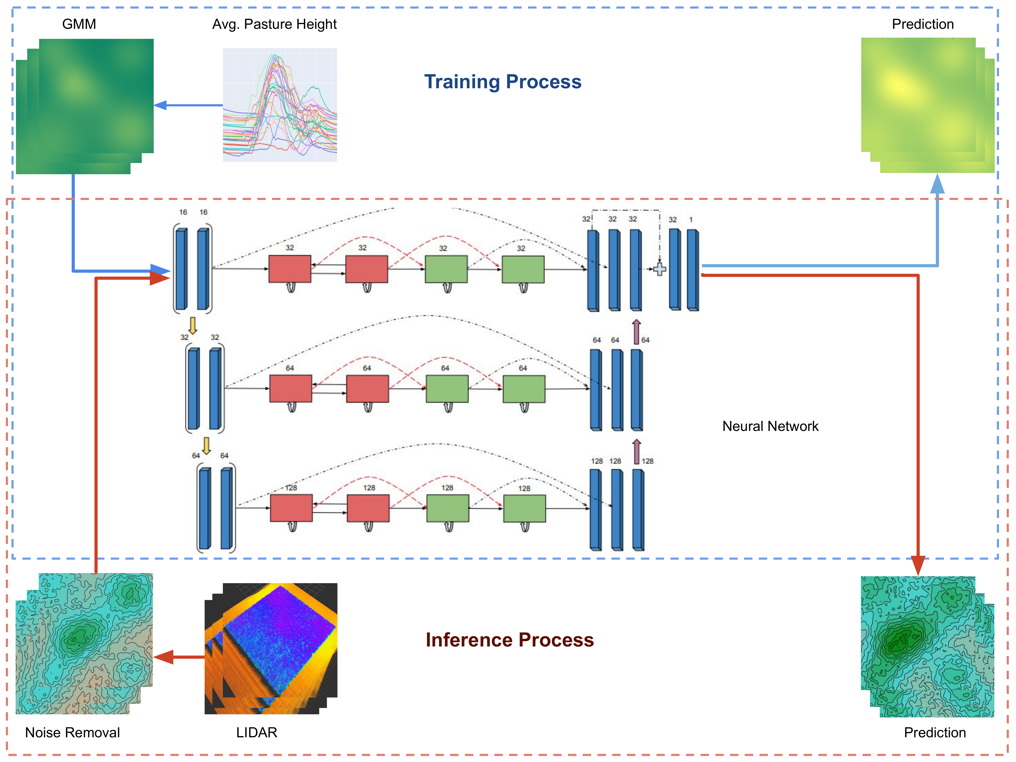
2.4. Data Processing for Training and Inference

First, in order to accommodate a truly scalable solution that is agnostic to the spatial dimensions of the pasture prediction problem, we train our model to predict on quantized patches of pastures and stitch the final prediction together. This methodology allows the model to accommodate varying pasture sizes for long-term predicts. Additionally, several other processing steps on the dataset are performed to improve the performance of the prediction model as described below:

• The use of convolution neural networks in deep learning introduces an unintended side effect popularly termed as boundary effects [47,48], where artifacts are introduced at the boundaries of the image due to no spatial information [49,50] available when CNN filters pass over boundaries of the image. We circumvent this issue by enlarging each image with size $\delta \le 100$, pixels through mirror padding [51] to add spatial information on the boundaries of each pasture image in the dataset $\mathcal{Z}\in {\mathbb{R}}^{100\times 100}$ updating our new training dataset to ${\mathcal{Z}}_{new}\in {\mathbb{R}}^{100+\delta \times 100+\delta }$.
• Training and inference of the neural network on original dimensions of the training dataset ${\mathcal{Z}}_{new}$ may potentially increase accuracy. However, it severely limits the capability of the neural network to adapt to variable input dimensions while also increasing computational requirements as GPU memory is a limited resource, specifically when training inputs with large dimensions. To this end, we quantize the training data ${\mathcal{Z}}_{new}\in {\mathbb{R}}^{100+\delta \times 100+\delta }$ into smaller sized patches of ${\mathcal{Z}}_q\in {\mathbb{R}}^{\delta \times \delta }$ with an overlap of $50\%$ between them. The overlapping of the images and subsequent reconstruction of the image post inference through a weighted average allows us to mitigate boundary effects between each cropped frame, an undesirable artifact of CNN output that would occur if they were to be naively cropped without any overlaps. This methodology requires the neural network to only learn over small patches of the field and can be practically used to predict field sizes of any size $N\times N$, as long as the original image is appropriately processed to meet the input size of $\delta \times \delta$, where $N\ge \delta$.
• We fix the sequence length of the training inputs and output prediction to trajectories of time $L_{in},L_{out}=15$. The final input training set is then defined as input sequences of ${\mathcal{Z}}_{in}=\left\{{\mathcal{Z}}_{in}^i|i=1,\dots ,\tau -L_{in}-L_{out}\right\}$, where $\tau$ is the number of data points in the quantized dataset ${\mathcal{Z}}_q$. Each individual sequence for the backward propagation is ${\mathcal{Z}}_{in}^i=\left\{Z_q^i,\dots ,Z_q^{i+L_{in}}\right\}$, where ${\mathcal{Z}}_{in}^i\in {\mathbb{R}}^{\delta \times \delta }$. Similarly, the target values dataset $\mathcal{Y}=\left\{{\mathcal{Y}}^i|i=1,\dots ,\tau -L_{in}-L_{out}\right\}$ is created for training. Each input sequence ${\mathcal{Z}}_{in}^i$ has a corresponding target value ${\mathcal{Y}}_{out}^i=\left\{Y_q^{i+1+L_{in}},\dots ,Y_q^{i+1+L_{in}+L_{out}}\right\}\in {\mathbb{R}}^{\delta \times \delta }$, where $Y_q^j=Z_q^j$.

2.5. Deep Learning Model for Long-Term Prediction

The choice of our architecture Figure 4 is primarily motivated by our goal of spatiotemporal learning. Recently, ConvLSTMs [34] have shown remarkable progress in learning representations and future frame predictions of video sequences, precipitation nowcasting, and also for classification problems of deforestation. A ConvLSTM can be simply defined as an LSTM recurrent network [52], with convolution operations replacing the matrix multiplication within an LSTM network as shown in Equation (2). LSTM networks are designed to process temporal dependencies by propagating its hidden state across time [33,39,52,53,54,55,56,57,58], or more simply, they transfer an aggregated history to allow future predictions to take advantage of the past. Similarly, the emergence of ConvLSTM is motivated by taking advantage of the temporal dependence of LSTMs and extending it as a spatiotemporal representation, making it an excellent choice for our application. The ConvLSTM architecture is defined as

$$\begin{array}{cc}\hfill i_t& =\sigma (W_{xi}\ast U^t+W_{hi}\ast H_{t-1}+W_{ci}\circ C_{t-1}+b_i),\hfill \\ \hfill f_t& =\sigma (W_{xf}\ast U^t+W_{hf}\ast U_{t-1}+W_{cf}\circ C_{t-1}+b_f),\hfill \\ \hfill C_t& =f_t\circ C_{t-1}+i_t\circ \tan \mathrm{h}(W_{xc}\ast U_t+W_{hc}\ast H_{t-1}+b_c),\hfill \\ \hfill o_t& =\sigma (W_{xo}\ast U^t+W_{ho}\ast H_{t-1}+W_{co}\circ C_t+b_o),\hfill \\ \hfill H_t& =o_t\circ tanh\left(C_t\right),\hfill \end{array}$$

(2)

where $U^t\in {\mathbb{R}}^{1\times d\times d}$ is an input to the ConvLSTM layer, $(H_1,\dots ,H_t)\in {\mathbb{R}}^{1\times d\times d}$, $(C_1,\dots C_t)\in {\mathbb{R}}^{1\times d\times d}$ are the hidden and cell states of the ConvLSTM cell, and $i_t,f_t,o_t\in {\mathbb{R}}^{1\times d\times d}$ are the interaction, forget, and output gates similar to an LSTM cell. The gates control the integration of information from the past and the present data to the next timestep. * is the convolution operation, and ∘ is the Hadamard Product [59].

In order to generate multi-step predictions, our architecture should be capable of identifying the underlying temporal patterns of available historical pasture growth $L_{in}$, and more so the spatial correlation within the pasture before generating predictions. To capture this spatiotemporal history, we introduce an encoder similar to the original ConvLSTM for precipitation nowcasting through radar data. However, we employ the use of Bi-ConvLSTM networks [60] similar to Bi-LSTMs [61], where we run two separate ConvLSTM networks each in the forward $(i\to i+L_{in})$ and reverse $(i+L_{in}\to i)$ direction of the input sequence. By learning the bi-direction temporal dependencies of pasture growth, we enable our model to achieve a better representation of time-series data. The hidden states of the ConvLSTM networks are then merged with a CNN operation at each timestep before being fed to the subsequent networks, $H_t=f^{bi}(H_t^f,H_t^b)$, where $f^{bi}$ is a CNN layer, and $H_t^f,H_t^b$ are the hidden states at time t of the ConvLSTM encoder in the forward and reverse direction, respectively. The encoder recursively parses the spatiotemporal information in the input sequence and generates an aggregated hidden representation in the final step, which is then used as a basis for forecasting future growth. This approach allows our network to generate richer representations specifically for learning the trends in sward height growth by encoding the history of pasture dynamics through the encoder.

A decoder framework is then implemented to enable the reconstruction of future predictions based on the aggregated historical hidden representations of the encoder. Since we do not have information for future time steps, we only use ConvLSTM networks processing the output sequence in the forward direction. The decoders copy the last hidden state of the encoder networks as their own initial state. The decoder utilizes its own output states as an input for future timesteps along with the hidden states of the encoder to recursively generate predictions for pasture heights.

Finally, to increase the representational power of the DeepPaSTL architecture, we use CNNs to pre-encode the inputs before feeding the recurrent encoder–decoder networks. Similarly, the outputs of the encoder–decoder are also parsed through CNNs to generate the final prediction. We implement the encoder–decoder framework across three spatial resolutions by down-sampling them by a factor of 2 with MaxPool layers [62] to allow the network to learn dependencies at different spatial representations, akin to the ubiquitous U-Net CNN framework [63]. Similar to [34], we use two sets of BiConvLSTM for each encoder and similarly two ConvLSTM decoders to independently learn the concept of distance and correlation within its neighborhood [64]. The representations at different spatial resolutions are finally merged together by up-sampling through CNNs. In order to improve training time, performance and negate the problem of vanishing gradients during training, we employ the use of residual connection [65,66,67,68], and batch normalization [69]. Residual connections from the pre-encoding to the post-encoding layers also help the network recreate the spatial context of the original images.

2.6. Uncertainty Estimation of the Model

Standard deep learning models that are trained through supervised learning do not estimate the uncertainty in its prediction. However, the paradigm of Bayesian Neural Networks (BNN) [24] enables the neural networks to estimate uncertainty in their outputs by evaluating the posterior distribution over its network weights. However, to model a large BNN, especially with the representational power required to forecast pasture growth, makes them computationally prohibitive. This is due to the fact that a full posterior distribution over the parameters of the neural network needs to be computed for each forward and backward pass. Recently, a computationally efficient method of approximating Bayesian inference [24] with the use of dropouts [40] was proposed. The key idea was to perform Markov Chain Monte Carlo (MCMC) sampling of the network parameters to generate stochastic inference of the network only in the forward pass. Dropouts in deep learning are more popularly used only during training to remove randomly sampled nodes from each layer l with a fixed probability $p^l$, to reduce overfitting and increase the robustness of the network by allowing each node to learn redundant and independent representations. However, Ref. [40] shows that introducing dropouts during inference enables the model to estimate uncertainty in its output. We utilize the approximate Bayesian inference in our model by introducing dropouts between each layer preceding the final output layer with $p^l=0.4$, and generate 500 samples of stochastic inference before estimating the average for the final prediction.

2.7. Experiment Details

In a brief comparison of different inputs of patch sizes, $\delta$ is used to compare the accuracy of the architecture as input size increases. The main limitation of the patch size is attributed to the limited GPU memory (VRAM) available for training. The input sizes can be increased as large as the available system capacity allows, although through our empirical evaluations, we observe that lower input sizes had better performance. Since it is quite unlikely that field measurements of pastures are available for every consecutive day, we compare results when the input observations are split apart every few days, i.e., $s=\{1,2,4\}$ time intervals between each input in the sequence. Additionally, having a larger s increases the effective time horizon of prediction, for example, for $s=4$ and $L_{out}=15$, and the model predicts 60 days into the future where every step is a progression of 4 days. We also perform comparisons to identify the architecture’s adaptability to missing data by performing imputation, wherein mean data are added between missing observations in the case of $s=\{2,4\}$. This helps simulate cases where field measurements might not be available due to severe weather conditions or resource constraints, and observe that the prediction model performs sufficiently well under these cases. To verify the effectiveness of the DeepPaSTL architecture, we evaluate our trained model on the simulated dataset in Section 2.2 and on 3D simulation of pasture environments in Gazebo with point cloud measurements as described in Section 2.3.

2.8. Model Training and Evaluation

Training and inference are performed for an input and output sequence of 15 steps, each using back-propagation through time (BPTT). However, it is to be noted that, due to the dynamic encoder–decoder framework, the architecture can use a variable sequence length during inference.The complete training and evaluation process is shown in Figure 5.

All models are trained with mean square error loss (MSE). Training is stopped when the validation loss does not improve for 10 consecutive epochs. Learning rates were individually tuned for each network by calculating the steepest gradient on a small sample dataset, although they usually were set to $3.5\times {10}^{-4}$. To test the model performance, we use the last two years of data $(2008,2009)$ for all evaluations in this study. The models are trained on 2x AMD Epyc 7742 CPUs and 8x Nvidia RTX 6000 GPUs with PyTorch as its back-end. Training time is generally 15 to 20 h for 30 epochs.

We evaluate the performance of our architecture with the following metrics: Root Mean Square Error (RMSE), Mean Absolute Error (MAE), Mean Absolute Percentage Error (MAPE), and average standard deviation of all predictions (aSt. Dev.), defined as

$$\begin{array}{cc}\hfill \mathrm{RMSE}& =\sqrt{\frac{1}{B}\times \sum _{i=1}^B{(Y_i-{\widehat{Y}}_i)}^2},\hfill \\ \hfill \mathrm{MAE}& =\frac{1}{B}\times \sum _{i=1}^B\left|Y_i-{\widehat{Y}}_i\right|,\hfill \\ \hfill \mathrm{MAPE}(\%)& =\frac{100}{B}\times \sum _{i=1}^B\left|\frac{Y_i-{\widehat{Y}}_i}{Y_i}\right|,\hfill \\ \hfill \mathrm{aSt}.\mathrm{Dev}.& =\sqrt{\frac{1}{B}\sum _{i=1}^{B}var\left({\widehat{Y}}_i\right)},\hfill \end{array}$$

where B is the number of output sequences, $Y_i$ is the ground truth, and ${\widehat{Y}}_i$ is the final prediction of the neural network after post-processing as described in Section 2.4.

3. Results

A comparison of the DeepPaSTL architecture over different spatial input sizes is performed on 3D pastures generated in Gazebo to understand the impact of quantization and spatial learning of the architecture. We then run our model for different observation or input intervals, s, to evaluate temporal dependencies. Additionally, we study how the imputation of missing data can impact the accuracy of the architecture when field measurements of the pastures are not available on a daily basis. Training losses are reported in Figure 6. Through our experimental results conducted both on the simulated data from GMM and the 3D pastures from Gazebo, we observe the following:

• DeepPaSTL predictions perform within a $15\%$ error rate for long horizon predictions up to 60 days in the future, and approximately with a $5\%$ error rate for predictions closer to its historical data.
• Allowing the model to have regular observations, i.e., with smaller intervals, is essential for capturing large dynamic changes in the pasture growth.
• DeepPaSTL prediction uncertainty increases as the volatility in pasture growth increases.
• We show that DeepPaSTL has the capacity to predict and generate future pasture terrains that replicate the growth and surface characteristics of ground truth data.

3.1. Effect of Input Quantization

We first compare the effect of the input quantization for interval $s=4$ and $\delta =\{32,64\}$ with uncertainty estimates as described in Section 2.6. The predicted sward heights for models trained with $\delta =64$ showed a slightly lower variability as compared to the smaller spatial size of the inputs with $\delta =32$. This larger variance in uncertainty for lower quantization is to be expected as the model has access to less spatial information. However, we do observe that, for the initial time horizon, the lower quantization $\delta =32$ significantly outperforms the larger $\delta =64$, Figure 7, while, as the number of steps in the output prediction increases, the error rates for $\delta =\{64,32\}$ are relatively similar. This is mainly attributed to the fact that the model with large spatial representations has an inherent advantage to perform better in a time period with fast-moving pasture dynamics, due to its extended capacity to learn spatial correlations of the evolving field. However, increasing the spatial size of the architecture makes it harder to train the network effectively to predict changes in the pasture. Pasture maps for the error $Y_i-{\widehat{Y}}_i$ and uncertainty in its prediction are shown in Figure 7. Through our empirical evaluations, we observe that the lower quantization of spatial inputs significantly outperformed,

Table 1. Accuracy scores are averaged for each testing dataset over the time period $(L_{\mathrm{in}}=L_{\mathrm{out}}=15)$. The following models were tested $(\delta =64,s=4)$, and $(\delta =32,s=\{1,2,4\left\}\right)$ with and without approximate Bayesian inference (MCMC) with 500 samples and $p^l=0.4$. Accuracy is then calculated both for the test set from 2008 to 2009, and the 30 days sequence of point cloud measurements from 3D pasture simulated in Gazebo. RMSE, MAE and aSt. Dev. values are reported in $\left(\mathrm{mm}\right)$ and MAPE in $(\%)$.

Model	Test Dataset (GMM)				3D Pasture (Gazebo)
	RMSE	MAE	MAPE	aSt. Dev.	RMSE	MAE	MAPE	aSt. Dev.
$(\delta =64,s=4)$ + MCMC	20.02	14.54	12.25	8.55	12.37	11.21	6.49	11.15
$(\delta =32,s=4)$ + MCMC	19.11	13.36	11.79	9.14	7.37	6.33	3.61	12.3
$(\delta =32,s=2)$ + MCMC	11.52	8.13	7.33	8.48	–	–	–	–
$(\delta =32,s=1)$ + MCMC	6.85	5.05	4.63	8.28	–	–	–	–
$(\delta =64,s=4)$	26.35	20.04	15.84	–	24.91	24.03	14.02	–
$(\delta =32,s=4)$	24.76	18.81	15.65	–	19.41	18.13	10.6	–
$(\delta =32,s=2)$	21.74	16.7	14.49	–	–	-	–	–
$(\delta =32,s=1)$	18.66	14.40	13.15	–	–	–	–	–

and Figure 7, and larger spatial input sizes, especially during the first half of the prediction horizon. This can be also be observed in the 3D Gazebo point cloud predictions where pasture growth rates were the highest for the initial time horizon, Figure 8a, Figure 9, Figure 10 and Figure 11. Therefore, we use $\delta =32$ for all future experiments, as the model can always update its predictions over time with new field measurements.

3.2. Effect of Intervals between Observations

We evaluate our architecture on varying input and output interval sizes of $s=\{1,2,4\}$, with a prediction horizon of $\{15,30,60\}$ days, respectively, and we observe that the accuracy of the architecture decreases as the number of intervals between each observation is increased. This can be clearly inferred from the training and validation loss for each model in Figure 6. Despite the accuracy loss, our model performs with a cumulative $88\%$ accuracy even in the most difficult pasture growth timelines for a 60-day prediction horizon. Trends in pasture growth exhibit a complicated pattern where there exists strong nonlinearity in growth pattern and large fluctuations over time. We observe that the accuracy across the prediction horizon averaged over the complete two-year testing dataset decreases drastically when the interval length is increased from 2 to 4, as shown in Table 1 and Figure 7. Moreover, we observe that the error rates follow the dynamic growth pattern of the pasture, where there is large growth in short periods of time, Figure 8a.

3.3. Uncertainty over Pasture Dynamics

Due to the volatile nature of pasture growth, it is imperative for prediction models to be capable of estimating uncertainty. Through stochastic inference by approximate Bayesian methods [40], we observe that the DeepPaSTL architecture has a higher uncertainty in its prediction at regions in the pasture with large growth dynamics (Figure 8). The model learns to predict regions with high sward heights quite accurately, as the model inherently captures these strong features within its spatial representations, and consequently we observe very low uncertainty in its prediction at high grass regions within the pasture. This is also partially attributed to the fact that peak pasture growths have a lower growth rate compared to pasture heights that are shorter. However, in the case of $s=4$, as we move forward in time towards the last prediction step at $i=8,10$, i.e., on the 32nd, and 40th day in the future, we observe that the confidence of the model drops as the time horizon increases, due to heavy pasture growth, and a sparse historical data (Figure 8b). It can be clearly observed that the average uncertainty increases, which is further exaggerated by the increased volatility in pasture growth. Moreover, under the approximate Bayesian inference due to repeated sampling and inference, the performance of the Bayesian DeepPaSTL model substantially outperforms the deterministic single pass inference that is used in standard deep learning methods (Figure 7). The MCMC sampling method allows the model to have a 3x improvement over standard single forward pass inferences over the short prediction horizon. It is to be noted that MCMC sampling with $s=\{1,2\}$ on average has an accuracy that is twice as good as the single forward pass methods. We attribute this improvement to the DeepPaSTLs capacity to accurately model the stochastic dynamics of the pasture by allowing different nodes in the network to dominate in each forward pass. We hypothesize that prioritizing on each individual node through stochastic sampling allows the model to regenerate precise dynamics of pasture growth by focusing on different factors and representations of the historical observations. However, for long horizon predictions of $s=4$, the difference in accuracy reduces as prediction steps get close to $L_{out}$, Figure 8b, which is attributed to a lack of observational data. We show the results for prediction performance with and without stochastic inference in Table 1, and Figure 7. Mean predictions for a 60-day horizon, mapped as a 3D field, is shown in Figure 12, with the example that has not been synthesized directly from the training data methodology.

3.4. Imputation of Missing Data

In order to improve the accuracy of the model for long horizon prediction near the $40+$ day mark and to address real-world applications that allow a reduction in the frequency of field measurements, we test the accuracy of the network when imputation is performed for missing data in the input sequence. We evaluate the performance of the models when under the following conditions: (a) When data are missing every other day, where an observation sequence of interval size $s=2$ is modified to fit a $s=1$ prediction model using an interpolation of the average growth between the missing data, (b) and similarly data available in four day intervals has three values inserted to predict with $s=1$ models. We then compare the results to a perfect model where data are available every day for $s=1$. We show that the network is robust to these events by adapting to the imputed data and manages to predict the future pasture sward heights to high accuracy,

Table 2. We measure the accuracy of the prediction model under missing observations over 2 years of the test data. We denote $x_t$ as the input that is missing and $Z_t$ as the available observation. $x_t$ is calculated by fitting a linear curve between the available observations within its interval. Evaluation is done for $(L_{\mathrm{in}}=L_{\mathrm{out}}=15)$ with $(\delta =32,s=1)$ with MCMC inference, using 500 samples and $p^l=0.4$. Accuracies are calculated for the test set generated with GMM from 2008 to 2009. RMSE, MAE and aSt. Dev. values are reported in $\left(\mathrm{mm}\right)$ and MAPE in $(\%)$.

Imputation	$(\mathit{\delta }=32,\mathit{s}=1)$ + MCMC
	RMSE	MAE	MAPE	aSt. Dev.
$Z_1,Z_2,\dots Z_{15}$	6.85	5.05	4.63	8.28
$Z_1,x_2,Z_3,x_4,\dots Z_{15}$	5.98	4.29	4.24	8.57
$Z_1,x_2,x_3,Z_4,x_5,x_6,\dots Z_{15}$	6.04	4.44	4.29	8.73

. We observe a modest improvement in the performance of model as the prediction network adapts to a gradual change of pasture growth from the interpolated data. This reinforces our assumption on the robustness of DeepPaSTL architecture and allows farm owners and enterprises to expend less resources on daily field measurements, saving valuable time and reducing the cost of operations of dairy-farms.

4. Discussion

This study demonstrates that the DeepPaSTL architecture accurately predicts pre-grazing pasture growths with an average error below $12\%$, using only the sward height measurements as its input. The experimental evaluations of this study highlight the capability of the DeepPaSTL architecture to implicitly learn the biological dependencies of pasture growths on climate variables such as precipitation, temperature, soil types, and pasture management processes among others. DeepPaSTL introduces a novel direction in pasture predictions by treating spatial measurements as the sole observation data for forecasting future pasture growths. The advantage of using this approach enables pasture farms to accurately predict future pasture evolution, even if they are not equipped to monitor fields on a regular schedule. Our results highlight the practical applicability of our method by depending only on high-resolution spatial mappings that can be generated through remote sensing, satellite imagery or UAVs. The proposed methodology in this study also provides a highly scalable prediction methodology that is adaptable to both small and large pastures.

Our results provide several insights on DeepPaSTL’s capability of predicting a highly dynamic spatiotemporal pasture over long horizons. Our approach exhibits excellent accuracy where mean errors were within $5\%$ for shorter time intervals s. For example, mean errors for $s=1$ were within $5\%$ across 2 years of the testing set, which is a substantial improvement over larger sequence intervals of $s=4$ with a cumulative accuracy of $12\%$, and a short horizon accuracy for the 20th day to be within $10\%$. Moreover, allowing the architecture to perform spatiotemporal predictions over smaller quantizations eases the prediction and learning burden of the network, further improving the accuracy. Lower quantizations of the model do not necessarily impact the prediction process, since inference times are negligible (usually less than an hour) when compared to pasture growth changes.

Bayesian inference, which combines the MCMC sampling to simulate a stochastic inference of the network, proved to be more robust than standard deep learning inference methods without uncertainty measurements. Inference through approximate Bayesian methods enabled the model to predict pasture growths with lower error, and more importantly, a strong correlation was observed between large errors and uncertainty in the predictions. The findings were indicative of correlations between the model’s capacity to understand the influence of spatiotemporal evolution through its observed data and its confidence in predicting large pasture height swings in a short period of time. The uncertainty is more pronounced when data are sparse especially, as s becomes larger.

The performance of the DeepPaSTL model may also be affected by several other factors that are not considered in this study due to the lack of available data. We simulate noise in LIDAR measurements of sward heights in the pasture through a Gaussian noise. Moreover, we also perform processing over these point cloud measurements to adapt the data to the neural network. These processes introduce bias and errors in the final prediction. Our synthetic dataset assumed five different varieties of grass; however, these might differ across the spatial field and other climatic and local factors that would change the dynamics of the input observations. This assumes that owners and enterprises are capable of adapting and controlling the variety of grass species in their environment to mitigate the issue of large divergences between training data and real-world measurements. However, the neural network can always be fine-tuned with newer observations and datasets to adapt to new pasture environments, and we expect the impact on the accuracy of the model to be modest.

Overall, our prediction results from the DeepPaSTL architecture emphasize several important directions that prediction and planning tools can consider for integration and future development. First, the DeepPaSTL encoder–decoder architecture presents a highly flexible tool for predicting pasture heights across varying spatial sizes and temporal observations. Second, we empirically show that synthetic datasets that are modeled appropriately can be a useful tool to generate training data for deep learning prediction models for pasture growths. Third, the accuracy of the predictions is correlated to the frequency of observations. However, the lack of intermediate field measurements can be mostly mitigated through apt use of data imputation. Finally, to allow deeper insights and increase the generalization power of the architecture, we hope to extend our work to a broader range of applications by including site-specific measurements and other climatic conditions, if available, as part of DeepPaSTL.

5. Conclusions

We prove the capabilities of modern deep learning techniques and algorithms for predicting pre-grazed pasture terrains for both long and short horizons. Through our proposed techniques, we aim to provide an important first step towards applying high resolution prediction methodologies over complete pasture terrains. Our DeepPaSTL modeling is capable of predicting over long horizons with an adequate degree of accuracy across both small and large pasture forms. As part of future work, we believe DeepPaSTL can be adapted to predict pasture regression due to grazing activities with minimal modifications. Since DeepPaSTL learns general trends in pasture growth rates, it can be directly applied to learn and predict growth of pastures recovering from grazing. A dual prediction model for recovery and regression of pastures due to grazing can be incorporated as part of planning systems, substantially reducing time and resources spent on field measurements. Adoption of these techniques can be accelerated by appropriate modeling of growth patterns of individual sites to generate synthetic historical datasets for DeepPaSTL to perform effectively across varied locations. Since DeepPaSTL can learn with new data accumulated over months, the model has an inherent capacity to effectively adapt to varying climatic and environmental conditions.

References

1. Garcia, S.C.; Clark, C.E.; Kerrisk, K.L.; Islam, M.R.; Fariña, S.; Evans, J. Gaps and variability in pasture utilisation in Australian pasture-based dairy systems. In Proceedings of the XXII International Grassland Congress (Revitalising Grasslands to Sustain Our Communities), Sydney, Australia, 15–19 September 2013; pp. 1709–1716. [Google Scholar]
2. Sala, O.E.; Paruelo, J.M.; Sala, O.E.; Paruelo, J.M. Ecosystem services in grasslands. In Nature’s Services: Societal Dependence on Natural Ecosystems; Island Press: Washington, DC, USA, 1997; pp. 237–251. [Google Scholar]
3. Insua, J.R.; Utsumi, S.A.; Basso, B. Estimation of spatial and temporal variability of pasture growth and digestibility in grazing rotations coupling unmanned aerial vehicle (UAV) with crop simulation models. PLoS ONE 2019, 14, e0212773. [Google Scholar] [CrossRef] [Green Version]
4. Fulkerson, W.; McKean, K.; Nandra, K.; Barchia, I. Benefits of accurately allocating feed on a daily basis to dairy cows grazing pasture. Aust. J. Exp. Agric. 2005, 45, 331–336. [Google Scholar] [CrossRef]
5. De Rosa, D.; Basso, B.; Fasiolo, M.; Friedl, J.; Fulkerson, B.; Grace, P.R.; Rowlings, D.W. Predicting pasture biomass using a statistical model and machine learning algorithm implemented with remotely sensed imagery. Comput. Electron. Agric. 2021, 180, 105880. [Google Scholar] [CrossRef]
6. Liu, J.; Williams, R.K. Submodular optimization for coupled task allocation and intermittent deployment problems. IEEE Robot. Autom. Lett. 2019, 4, 3169–3176. [Google Scholar]
7. Liu, J.; Williams, R.K. Monitoring over the long term: Intermittent deployment and sensing strategies for multi-robot teams. In Proceedings of the IEEE International Conference on Robotics and Automation, Paris, France, 31 May 2020; pp. 7733–7739. [Google Scholar]
8. Sung, Y.; Budhiraja, A.K.; Williams, R.K.; Tokekar, P. Distributed assignment with limited communication for multi-robot multi-target tracking. Auton. Robots 2010, 44, 57–73. [Google Scholar] [CrossRef] [Green Version]
9. Heintzman, L.; Williams, R.K. Multi-agent intermittent interaction planning via sequential greedy selections over position samples. IEEE Robot. Autom. Lett. 2021, 6, 534–541. [Google Scholar] [CrossRef]
10. Heintzman, L.; Hashimoto, A.; Abaid, N.; Williams, R.K. Anticipatory Planning and Dynamic Lost Person Models for Human-Robot Search and Rescue. In Proceedings of the IEEE International Conference on Robotics and Automation, Xi’an, China, 30 May 2021; pp. 8252–8258. [Google Scholar]
11. Liu, J.; Williams, R.K. Coupled temporal and spatial environment monitoring for multi-agent teams in precision farming. In Proceedings of the IEEE Conference on Control Technology and Applications, Montreal, QC, Canada, 24–26 August 2020; pp. 273–278. [Google Scholar]
12. Liu, J.; Williams, R.K. Optimal intermittent deployment and sensor selection for environmental sensing with multi-robot teams. In Proceedings of the IEEE International Conference on Robotics and Automation, Brisbane, Australia, 21–25 May 2018; pp. 1078–1083. [Google Scholar]
13. Williams, R.K.; Gasparri, A.; Ulivi, G. Decentralized matroid optimization for topology constraints in multi-robot allocation problems. In Proceedings of the IEEE International Conference on Robotics and Automation, Marina Bay Sands, Singapore, 29 May 2017; pp. 293–300. [Google Scholar]
14. Tao, F.; Yokozawa, M.; Zhang, Z. Modelling the impacts of weather and climate variability on crop productivity over a large area: A new process-based model development, optimization, and uncertainties analysis. Agric. For. Meteorol. 2009, 149, 831–850. [Google Scholar] [CrossRef]
15. Iizumi, T.; Yokozawa, M.; Nishimori, M. Parameter estimation and uncertainty analysis of a large-scale crop model for paddy rice: Application of a Bayesian approach. Agric. For. Meteorol. 2009, 149, 333–348. [Google Scholar] [CrossRef]
16. Lobell, D.B.; Burke, M.B. On the use of statistical models to predict crop yield responses to climate change. Agric. For. Meteorol. 2010, 150, 1443–1452. [Google Scholar] [CrossRef]
17. Chen, Y.; Guerschman, J.; Shendryk, Y.; Henry, D.; Harrison, M.T. Estimating Pasture Biomass Using Sentinel-2 Imagery and Machine Learning. Remote Sens. 2021, 13, 603. [Google Scholar] [CrossRef]
18. Gargiulo, J.; Clark, C.; Lyons, N.; de Veyrac, G.; Beale, P.; Garcia, S. Spatial and temporal pasture biomass estimation integrating electronic plate meter, planet cubesats and sentinel-2 satellite data. Remote Sens. 2020, 12, 3222. [Google Scholar] [CrossRef]
19. Ali, I.; Greifeneder, F.; Stamenkovic, J.; Neumann, M.; Notarnicola, C. Review of machine learning approaches for biomass and soil moisture retrievals from remote sensing data. Remote Sens. 2015, 7, 16398–16421. [Google Scholar]
20. Dang, A.T.N.; Nandy, S.; Srinet, R.; Luong, N.V.; Ghosh, S.; Kumar, A.S. Forest aboveground biomass estimation using machine learning regression algorithm in Yok Don National Park, Vietnam. Ecol. Inform. 2019, 50, 24–32. [Google Scholar] [CrossRef]
21. Ghosh, S.M.; Behera, M.D. Aboveground biomass estimation using multi-sensor data synergy and machine learning algorithms in a dense tropical forest. Appl. Geogr. 2018, 96, 29–40. [Google Scholar] [CrossRef]
22. Rangwala, M.; Williams, R. Learning Multi-Agent Communication through Structured Attentive Reasoning. Adv. Neural Inf. Process. Syst. 2020, 33, 10088–10098. [Google Scholar]
23. Wehbe, R.; Williams, R.K. A Deep Learning Approach for Probabilistic Security in Multi-Robot Teams. IEEE Robot. Autom. Lett. 2019, 4, 4262–4269. [Google Scholar] [CrossRef]
24. Neal, R.M. Bayesian Learning for Neural Networks; Springer Science & Business Media: Berlin/Heidelberg, Germany, 2012; Volume 118. [Google Scholar]
25. Fukushima, K.; Miyake, S. Neocognitron: A self-organizing neural network model for a mechanism of visual pattern recognition. In Competition and Cooperation in Neural Nets; Springer: Berlin/Heidelberg, Germany, 1982; pp. 267–285. [Google Scholar]
26. LeCun, Y.; Haffner, P.; Bottou, L.; Bengio, Y. Object recognition with gradient-based learning. In Shape, Contour and Grouping in Computer Vision; Springer: Berlin/Heidelberg, Germany, 1999; pp. 319–345. [Google Scholar]
27. Lin, Z.; Li, M.; Zheng, Z.; Cheng, Y.; Yuan, C. Self-attention convlstm for spatiotemporal prediction. In Proceedings of the AAAI Conference on Artificial Intelligence, New York, NY, USA, 7 February 2020; Volume 34, pp. 11531–11538. [Google Scholar]
28. Xu, Y.; Gao, L.; Tian, K.; Zhou, S.; Sun, H. Non-local convlstm for video compression artifact reduction. In Proceedings of the IEEE/CVF International Conference on Computer Vision, Seoul, Korea, 27 October 2019; pp. 7043–7052. [Google Scholar]
29. Azad, R.; Asadi-Aghbolaghi, M.; Fathy, M.; Escalera, S. Bi-directional ConvLSTM U-Net with densley connected convolutions. In Proceedings of the IEEE/CVF International Conference on Computer Vision Workshops, Seoul, Korea, 27 October 2019; pp. 406–415. [Google Scholar]
30. Xu, N.; Yang, L.; Fan, Y.; Yang, J.; Yue, D.; Liang, Y.; Price, B.; Cohen, S.; Huang, T. Youtube-vos: Sequence-to-sequence video object segmentation. In Proceedings of the European Conference on Computer Vision (ECCV), Munich, Germany, 8–14 September 2018; pp. 585–601. [Google Scholar]
31. Oliu, M.; Selva, J.; Escalera, S. Folded recurrent neural networks for future video prediction. In Proceedings of the European Conference on Computer Vision, Munich, Germany, 8–14 September 2018; pp. 716–731. [Google Scholar]
32. Michalski, V.; Memisevic, R.; Konda, K. Modeling deep temporal dependencies with recurrent grammar cells. Adv. Neural Inf. Process. Syst. 2014, 27, 1925–1933. [Google Scholar]
33. Srivastava, N.; Mansimov, E.; Salakhudinov, R. Unsupervised learning of video representations using lstms. In Proceedings of the International Conference on Machine Learning, PMLR, Lile, France, 6–11 July 2015; pp. 843–852. [Google Scholar]
34. Xingjian, S.; Chen, Z.; Wang, H.; Yeung, D.Y.; Wong, W.K.; Woo, W.c. Convolutional LSTM network: A machine learning approach for precipitation nowcasting. In Proceedings of the Advances in Neural Information Processing Systems, Montreal, QC, Canada, 7–12 December 2015; pp. 802–810. [Google Scholar]
35. Lotter, W.; Kreiman, G.; Cox, D. Deep predictive coding networks for video prediction and unsupervised learning. arXiv 2016, arXiv:1605.08104. [Google Scholar]
36. Wang, Y.; Long, M.; Wang, J.; Gao, Z.; Yu, P.S. Predrnn: Recurrent neural networks for predictive learning using spatiotemporal lstms. In Proceedings of the International Conference on Neural Information Processing Systems, Long Beach, CA, USA, 4–9 December 2017; pp. 879–888. [Google Scholar]
37. Wang, Y.; Gao, Z.; Long, M.; Wang, J.; Philip, S.Y. Predrnn++: Towards a resolution of the deep-in-time dilemma in spatiotemporal predictive learning. In Proceedings of the International Conference on Machine Learning, PMLR, Stockholm, Sweden, 10–15 July 2018; pp. 5123–5132. [Google Scholar]
38. Koenig, N.; Howard, A. Design and use paradigms for gazebo, an open-source multi-robot simulator. In Proceedings of the 2004 IEEE/RSJ International Conference on Intelligent Robots and Systems (IROS)(IEEE Cat. No. 04CH37566), Sendai, Japan, 28 September 2004; Volume 3, pp. 2149–2154. [Google Scholar]
39. Sutskever, I.; Vinyals, O.; Le, Q.V. Sequence to sequence learning with neural networks. In Proceedings of the Advances in Neural Information Processing Systems, Montreal, QC, Canada, 12–13 December 2014; pp. 3104–3112. [Google Scholar]
40. Gal, Y.; Ghahramani, Z. Dropout as a bayesian approximation: Representing model uncertainty in deep learning. In Proceedings of the International Conference on Machine Learning, PMLR, New York, NY, USA, 19–24 June 2016; pp. 1050–1059. [Google Scholar]
41. Archontoulis, S.V.; Miguez, F.E.; Moore, K.J. Evaluating APSIM Maize, Soil Water, Soil Nitrogen, Manure, and Soil Temperature Modules in the Midwestern United States. Agron. J. 2014, 106, 1025–1040. [Google Scholar] [CrossRef]
42. Li, F.; Newton, P.; Lieffering, M. Testing simulations of intra- and inter-annual variation in the plant production response to elevated CO2 against measurements from an 11-year FACE experiment on grazed pasture. Glob. Chang. Biol. 2013, 20, 228–239. [Google Scholar] [CrossRef] [PubMed]
43. Liu, J.; Zhou, L.; Tokekar, P.; Williams, R.K. Distributed Resilient Submodular Action Selection in Adversarial Environments. IEEE Robot. Autom. Lett. 2021, 6, 5832–5839. [Google Scholar] [CrossRef]
44. Wehbe, R.; Williams, R.K. Probabilistic Resilience of Dynamic Multi-Robot Systems. IEEE Robot. Autom. Lett. 2021, 6, 1777–1784. [Google Scholar]
45. Heintzman, L.; Williams, R.K. Nonlinear observability of unicycle multi-robot teams subject to nonuniform environmental disturbances. Auton. Robot. 2020, 44, 1149–1166. [Google Scholar] [CrossRef]
46. Wehbe, R.; Williams, R.K. Probabilistic Security for Multirobot Systems. IEEE Trans. Rob. 2021, 37, 146–165. [Google Scholar] [CrossRef]
47. Innamorati, C.; Ritschel, T.; Weyrich, T.; Mitra, N.J. Learning on the edge: Explicit boundary handling in cnns. arXiv 2018, arXiv:1805.03106. [Google Scholar]
48. Innamorati, C.; Ritschel, T.; Weyrich, T.; Mitra, N.J. Learning on the edge: Investigating boundary filters in cnns. Int. J. Comput. Vis. 2019, 128, 773–782. [Google Scholar] [CrossRef] [Green Version]
49. Hashemi, M. Enlarging smaller images before inputting into convolutional neural network: Zero-padding vs. interpolation. J. Big Data 2019, 6, 1–13. [Google Scholar] [CrossRef]
50. Albawi, S.; Mohammed, T.A.; Al-Zawi, S. Understanding of a convolutional neural network. In Proceedings of the International Conference on Engineering and Technology, Antalya, Turkey, 21–23 August 2017; pp. 1–6. [Google Scholar]
51. Tang, H.; Ortis, A.; Battiato, S. The impact of padding on image classification by using pre-trained convolutional neural networks. In Proceedings of the International Conference on Image Analysis and Processing, Trento, Italy, 9–13 September 2019; Springer: Berlin/Heidelberg, Germany, 2019; pp. 337–344. [Google Scholar]
52. Hochreiter, S.; Schmidhuber, J. Long short-term memory. Neural Comput. 1997, 9, 1735–1780. [Google Scholar]
53. Graves, A. Generating sequences with recurrent neural networks. arXiv 2013, arXiv:1308.0850. [Google Scholar]
54. Cho, K.; Van Merriënboer, B.; Gulcehre, C.; Bahdanau, D.; Bougares, F.; Schwenk, H.; Bengio, Y. Learning phrase representations using RNN encoder–decoder for statistical machine translation. arXiv 2014, arXiv:1406.1078. [Google Scholar]
55. Donahue, J.; Anne Hendricks, L.; Guadarrama, S.; Rohrbach, M.; Venugopalan, S.; Saenko, K.; Darrell, T. Long-term recurrent convolutional networks for visual recognition and description. In Proceedings of the IEEE Conference on Computer Vision and Pattern Recognition, Boston, MA, USA, 8–10 June 2015; pp. 2625–2634. [Google Scholar]
56. Karpathy, A.; Fei-Fei, L. Deep visual-semantic alignments for generating image descriptions. In Proceedings of the IEEE Conference on Computer Vision and Pattern Recognition, Boston, MA, USA, 8–10 June 2015; pp. 3128–3137. [Google Scholar]
57. Ranzato, M.; Szlam, A.; Bruna, J.; Mathieu, M.; Collobert, R.; Chopra, S. Video (language) modeling: A baseline for generative models of natural videos. arXiv 2014, arXiv:1412.6604. [Google Scholar]
58. Xu, K.; Ba, J.; Kiros, R.; Cho, K.; Courville, A.; Salakhudinov, R.; Zemel, R.; Bengio, Y. Show, attend and tell: Neural image caption generation with visual attention. In Proceedings of the International Conference on Machine Learning, PMLR, Lille, France, 6–11 July 2015; pp. 2048–2057. [Google Scholar]
59. Horn, R.A. The hadamard product. Proc. Symp. Appl. Math. 1990, 40, 87–169. [Google Scholar]
60. Song, H.; Wang, W.; Zhao, S.; Shen, J.; Lam, K.M. Pyramid dilated deeper convlstm for video salient object detection. In Proceedings of the European Conference on Computer Vision (ECCV), Munich, Germany, 8–14 September 2018; pp. 715–731. [Google Scholar]
61. Graves, A.; Schmidhuber, J. Framewise phoneme classification with bidirectional LSTM and other neural network architectures. Neural Netw. 2005, 18, 602–610. [Google Scholar] [CrossRef]
62. Simonyan, K.; Zisserman, A. Very deep convolutional networks for large-scale image recognition. arXiv 2014, arXiv:1409.1556. [Google Scholar]
63. Ronneberger, O.; Fischer, P.; Brox, T. U-net: Convolutional networks for biomedical image segmentation. In Proceedings of the International Conference on Medical image Computing and Computer-Assisted Intervention, Munich, Germany, 5–9 October 2015; Springer: Berlin/Heidelberg, Germany, 2015; pp. 234–241. [Google Scholar]
64. Zhang, J.; Zheng, Y.; Qi, D.; Li, R.; Yi, X. DNN-based prediction model for spatio-temporal data. In Proceedings of the International Conference on Advances in Geographic Information Systems, Burlingame, CA, USA, 31 October 2016; pp. 1–4. [Google Scholar]
65. Srivastava, R.K.; Greff, K.; Schmidhuber, J. Training very deep networks. arXiv 2015, arXiv:1507.06228. [Google Scholar]
66. He, K.; Zhang, X.; Ren, S.; Sun, J. Deep residual learning for image recognition. In Proceedings of the IEEE Conference on Computer Vision and Pattern Recognition, Las Vegas, NV, USA, 23–30 June 2016; pp. 770–778. [Google Scholar]
67. He, K.; Zhang, X.; Ren, S.; Sun, J. Identity mappings in deep residual networks. In Proceedings of the European Conference on Computer Vision, Amsterdam, The Netherlands, 11–14 October 2016; Springer: Berlin/Heidelberg, Germany, 2016; pp. 630–645. [Google Scholar]
68. Huang, G.; Liu, Z.; Van Der Maaten, L.; Weinberger, K.Q. Densely connected convolutional networks. In Proceedings of the IEEE Conference on Computer Vision and Pattern Recognition, Honolulu, HI, USA, 21–26 July 2017; pp. 4700–4708. [Google Scholar]
69. Ioffe, S.; Szegedy, C. Batch normalization: Accelerating deep network training by reducing internal covariate shift. In Proceedings of the International Conference on Machine Learning, PMLR, Lille, France, 6–11 July 2015; pp. 448–456. [Google Scholar]
Figure 1. (a) Average pasture height and (b) mean and standard deviation of the 30 years of historical data across three sites in Iowa from APSIMs Met module are shown for each day of the year.
Agronomy 11 02245 g001
Figure 2. Grass models generated in Gazebo to populate the pasture terrain.
Agronomy 11 02245 g002
Figure 3. (a) Gazebo point cloud surface as measured in Gazebo with a hector quad-copter equipped with LIDAR; (b) raw measurements (mm) on the Gazebo point cloud in (a) in a contour plot; (c) processed (filtered) measurements (mm) adapted for neural network predictions.
Agronomy 11 02245 g003
Figure 4. Encoder–decoder architecture with ConvLSTM and residual connections (example for 32 × 32 pixels in the lowest resolution). The encoder consists of the two initial 2D convolution layers that extract the initial features of the input. Subsequently, the BiConvLSTM encoders are deployed to learn the forward and backward correlations over these extracted features of the input sequence. The ConvLSTM decoder then recursively unwraps the hidden features encoded in the hidden state of the encoder, and the 2D convolution layers map it to output predictions. The number of feature maps of each CNN layer is denoted above their respective blocks.
Agronomy 11 02245 g004
Figure 5. Process for training and inference of DeepPaSTL. Synthetic training datasets are created using GMM models based on the average pasture heights of Iowa sites. Real world field measurements can be obtained by using LIDAR point cloud measurements. The point cloud data are then processed to smooth out sensor noise and then DeepPaSTL is used to predict future pasture heights.
Agronomy 11 02245 g005
Figure 6. Training and Validation (MSE) Losses for 30 epochs for models trained with δ = 64 , s = 4 and δ = 32 , s = { 1 , 2 , 4 } . We observe that the loss rates are correlated to the observation intervals for input sequence. This is attributed to the fact that the architecture’s prediction performance is heavily dependent on recognizing temporal patterns in pasture growth due to the highly dynamic nature of pasture evolution.
Agronomy 11 02245 g006
Figure 7. Mean absolute percentage error across all the data points consisting of two years in the test set (GMM) for (a) models without MCMC sampling, and (b) models with MCMC sampling. MAPE and standard deviation are averaged over all the coordinates of the pasture, and the prediction step for different models. We observe that, as s increases, the errors increase over the prediction horizon. s = 4 , 2 , 1 effectively correlate to 60, 30, and 15 day prediction horizons.
Agronomy 11 02245 g007
Figure 8. Prediction (a) Error vs Prediction Step ( mm ) and (b) Standard Deviation vs Prediction Step ( mm ) bands for 50 % , 75 % , 25 % quantile range for δ = { 32 , 64 } , s = 4 for a 10 m × 10 m pasture for L o u t = { 1 , 6 , 11 , 15 } , respectively, and ground truth prediction from the 3D Pasture generated in Gazebo depicting the rate of change of pastures over 60 days. We observe that the lower quantization δ = 32 outperforms the larger input quantization over the complete predicted time period.
Agronomy 11 02245 g008
Figure 9. Prediction average height ( mm ) using approximate Bayesian inference for δ = { 32 , 64 } , s = 4 for a 10 m × 10 m pasture for L o u t = { 1 , 6 , 11 , 15 } , respectively. Input sequence to the DeepPaSTL network L i n = 15 is 01 April 2019 to 27 May 2019 and output prediction L o u t = 15 every 4 days. The predictions are 1 , 24 , 44 , 60 days in the future during the peak pasture growth time of 31 May 2019 to 26 July 2019. (Top) Target values acquired from point cloud measurements with LIDAR of 3D pasture generated in Gazebo. (Middle) δ = 64 generally underestimates the growth of the pasture resulting in larger errors; however, it generally has a better tracking for lower lying areas or receding pasture heights especially for the longer horizon. (Bottom) δ = 32 The lower quantization tracks the peaks and troughs of the sward height measurements quite accurately for the near horizon.
Agronomy 11 02245 g009
Figure 10. Prediction errors ( mm ) for δ = { 32 , 64 } , s = 4 for a 10 m × 10 m pasture for L o u t = { 1 , 6 , 11 , 15 } respectively. Input sequence to the DeepPaSTL network L i n = 15 is 01 April 2019 to 27 May 2019 and output prediction L o u t = 15 every 4 days. These error maps effectively correlate to 1 , 24 , 44 , 60 days in the future during the peak pasture growth time of 31 May 2019 to 26 July 2019. (Bottom) δ = 32 We observe that the lower quantization of the pasture has a distinct advantage through reduced prediction errors as compared to (Top) δ = 64 for the same set of inputs.
Agronomy 11 02245 g010
Figure 11. Standard deviation ( mm ) of predictions for δ = { 32 , 64 } , s = 4 for a 10 m × 10 m pasture for L o u t = { 1 , 6 , 11 , 15 } , respectively. We observe lower uncertainties at the peaks of the pasture due to its lower variability over time. Input sequence to the DeepPaSTL network L i n = 15 is 01 April 2019 to 27 May 2019 and output prediction L o u t = 15 every 4 days. The uncertainty estimates effectively correlate to 1 , 24 , 44 , 60 days in the future during the peak pasture growth time of 31 May 2019 to 26 July 2019. (Bottom) δ = 32 We observe the lower quantization of the pasture has higher uncertainty in its prediction when less spatial information is available for processing especially when pasture dynamics are high. (Top) δ = 64 has smaller prediction uncertainties for the same set of inputs.
Agronomy 11 02245 g011
Figure 12. An example of 3D predicted pastures from the Gazebo simulated point cloud measurements for s = 4 . (Top) Ground truth measured sward heights ( mm ) of the pasture. Left to right for a 60-day prediction horizon shown for every 8th day. (Bottom) Prediction by a δ = 32 , s = 4 model.
Agronomy 11 02245 g012