Simulating Canopy Temperature Using a Random Forest Model to Calculate the Crop Water Stress Index of Chinese Brassica

Abstract

The determination of crop water status has positive effects on the Chinese Brassica industry and irrigation decisions. Drought can decrease the production of Chinese Brassica, whereas over-irrigation can waste water. It is desirable to schedule irrigation when the crop suffers from water stress. In this study, a random forest model was developed using sample data derived from meteorological measurements including air temperature (Ta), relative humidity (RH), wind speed (WS), and photosynthetic active radiation (Par) to predict the lower baseline ($T_{wet}$) and upper baseline ($T_{dry}$) canopy temperatures for Chinese Brassica from 27 November to 31 December 2020 (E1) and from 25 May to 20 June 2021 (E2). Crop water stress index (CWSI) values were determined based on the predicted canopy temperature and used to assess the crop water status. The study demonstrated the viability of using a random forest model to forecast $T_{wet}$ and $T_{dry}$. The coefficients of determination (R²) in E1 were 0.90 and 0.88 for development and 0.80 and 0.77 for validation, respectively. The R² values in E2 were 0.91 and 0.89 for development and 0.83 and 0.80 for validation, respectively. Our results reveal that the measured and predicted CWSI values had similar R² values related to stomatal conductance (~0.5 in E1, ~0.6 in E2), whereas the CWSI showed a poor correlation with transpiration rate (~0.25 in E1, ~0.2 in E2). Finally, the methodology used to calculate the daily CWSI for Chinese Brassica in this study showed that both $T_{wet}$ and $T_{dry}$, which require frequent measuring and design experiment due to the trial site and condition changes, have the potential to simulate environmental parameters and can therefore be applied to conveniently calculate the CWSI.

1. Introduction

Chinese Brassica (Brassica chinensis L. var. parachinensis (Bailey)) has high nutritional value and is a critical vegetable for the Chinese population whose diet consists largely of vegetables in the Guangdong province of China, and Chinese Brassica is one of the highest produced vegetables in Guangdong province [1]. During the growing process, Chinese Brassica is susceptible to soil water deficiency, which affects its ability to undergo photosynthesis and stomatal movements and eventually leads to a decrease in yield [2]. The use of a suitable irrigation strategy concerning the time to trigger irrigation can enhance water use efficiency and crop productivity [3]. It has been argued that the principal beneficiary of irrigation is the crop, rather than the soil [4]; consequently, the irrigation strategy should be formulated according to the water status of the crops. Several crop-based indicators, including stomatal conductance, stem water potential, and canopy temperature, have been introduced to detect crop water status [5]. As the channel of gas exchange, the stomata are sensitive and their conductance declines dramatically when the crop is suffering from water stress [6,7,8]. Stem water potential has also been used to characterize crop water stress, showing a good correlation [9,10]. However, these measurements are time-consuming and leaf-destructive. With the rapid development of thermal infrared technology, the use of the canopy temperature as a metric has the merits of quick measurement [11], explicit results [12], and a lack of damage to the plants [13]. It has also been shown to have a significantly negative relationship with the stomata; therefore, canopy temperature is a good indicator of water stress [14,15,16]. However, methods which utilize canopy temperature to describe crop water status are highly variable and unstable [12,16]. Additionally, canopy temperature alone does not immediately change with water status, which needs to be normalized to the environmental conditions [17].

The Crop Water Stress Index (CWSI), proposed in 1981, is derived from the canopy temperature. It has been widely applied to assess water status and schedule irrigation regimes [18,19,20,21]. Theoretically, the CWSI ranges from 0 to 1, where the maximum value of 1 indicates that the crop has sufficient water, whereas the minimum value of 0 indicates that the crop has an extreme water deficit. The CWSI is not only used to quantify the water stress gradient; the majority of studies have revealed that it has a strong association with a series of physical activities related to the crop, such as stomatal conductance, transpiration rate, and stem water potential [16,22,23]. Generally, the CWSI is calculated via empirical and theoretical methods, with the empirical formula being easier and quicker to use. CWSI values obtained using the theoretical method based on energy balance are relatively precise. However, the data collection and calculation methods involved are arduous and complex [24].

The main task of the empirical equation is to determine the lower and upper baseline canopy temperatures using the crop canopy temperature, air temperature, and relative humidity. Previous studies have developed different ways of obtaining the lower and upper baseline temperatures to refine the empirical formula. For example, multiple studies have clearly demonstrated the CWSI method, in which the lower limit is based on a linear equation between the vapor pressure difference (VPD) and the well-watered canopy temperature can effectively indicate crop water stress. This has been demonstrated in cotton [24], pepper [25], grape [26], and olive [14] crops. However, Idso et al. [27] consider VPD to be influenced by the environment because it changes with the season, region, and crop growth process, making it challenging to create an equation. Using the canopy temperature of a well-watered plantation to determine the lower baseline temperature has been proven to be a viable method for sugar beet [28], Indian mustard [29], grape [30], and olive [31] crops.

With respect to the upper baseline, many researchers have applied a constant. Irmak et al. [32] designed different water treatments for maize and found that the average canopy temperature was always 5.0 °C above the air temperature when maize was under severe water stress, and suggested that the air temperature plus a constant could be taken as the upper baseline for the canopy temperature to simplify the calculation. Considering this conclusion, previous studies have used the air temperature plus 5.0 °C to represent the upper baseline of corn [33] and olive [31] crops, and others have used the air temperature plus 2.0, 3.0, or 7.0 °C based on their experiments [29,34,35]. It has been shown that different crops may require distinct methods. Rather than applying the average value, Cristina et al. [21] and Gonzalez et al. [36] took the maximum canopy temperature under conditions of severe stress as the upper baseline for citrus and demonstrated an excellent correlation between the CWSI and stem water potential. Certainly, the lower and upper baseline canopy temperatures must be measured.

Predictions using easily attainable data allow canopy temperatures and CWSI values to be obtained more quickly and conveniently. King et al. [37] utilized a neural network to estimate the canopy temperature of well-watered crops based on air temperature, relative humidity, wind speed, and solar radiation. The results indicated that the neural network performed well regarding the estimation and viability of canopy temperature simulation using a considerable amount of previous environmental data. Kumar et al. [29] constructed two neural network models and obtained the canopy temperature, air temperature, and relative humidity, which were then used to predict CWSI values in order to avoid calculating the lower and upper baseline temperatures. To our knowledge, no studies have predicted the lower and upper baseline values using environmental factors at the same time. The canopy temperature is affected by the air temperature, relative humidity, wind speed, and solar radiation [38]. When solar radiation increases, the canopy temperature changes evidently, increasing at a rapid rate [31,39]. Photosynthetic active radiation (Par), a portion of solar radiation absorbed by the photosynthetic system of crops, plays a critical role in providing energy to support photosynthetic processes related to the conversion of radiation energy into chemical energy [40]. However, Par has not been considered for canopy temperature simulation in similar studies. It is noteworthy that the environmental conditions mentioned above are easy to replicate and monitor.

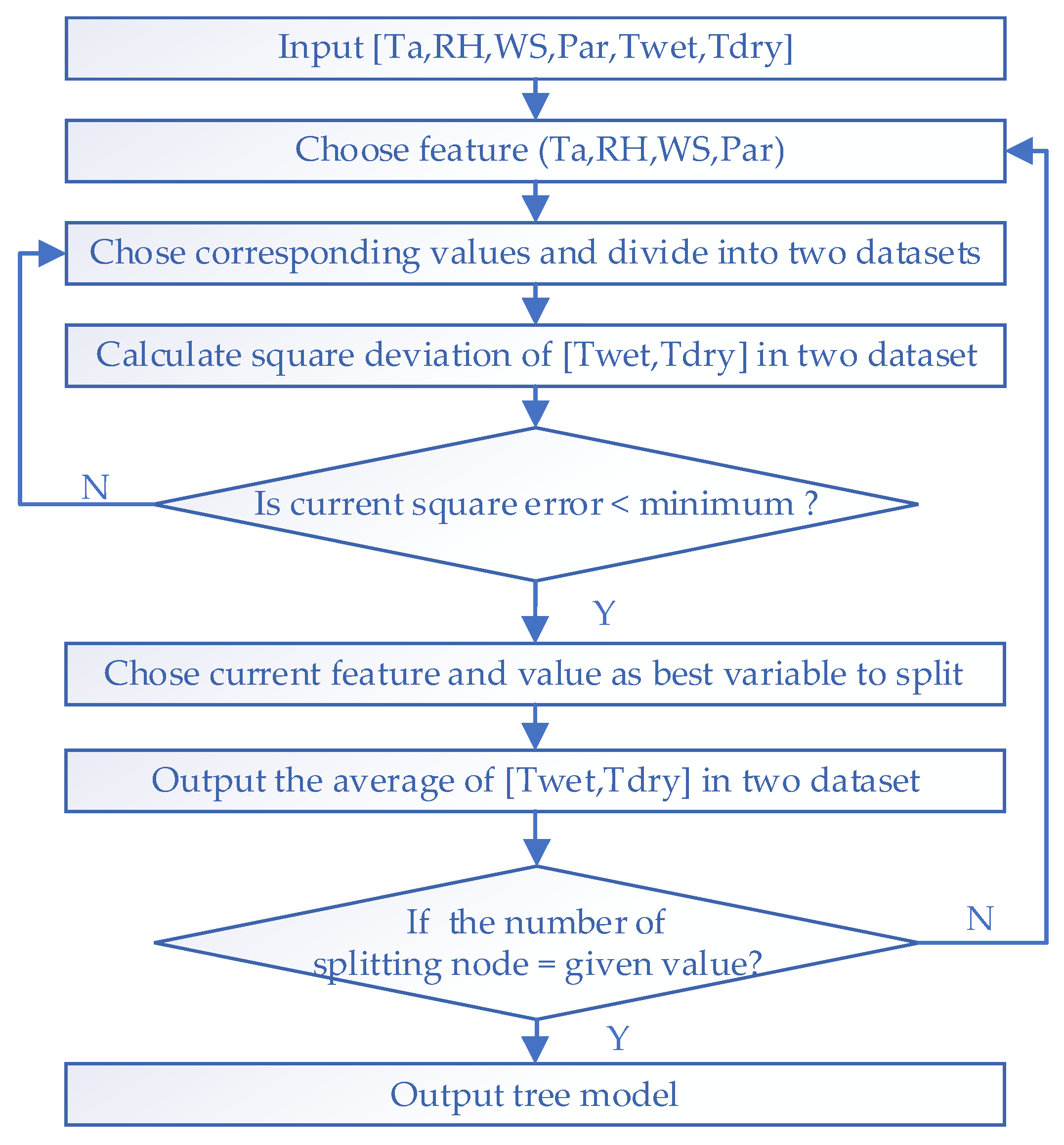
The random forest (RF) model has been applied successfully to predict agricultural information, for example, soil temperature [41], soil moisture content [42,43], and crop yield [44,45]. Usually, a RF model consists of numerous decision trees. The tree numbers are randomly distributed, and the final prediction is the weighted mean of all trees. During the decision tree building process, a dataset is continually split with definite regularity using the best feature and value. It is eventually divided into different subsets to represent categories. The advantages over using a single decision tree are that the RF model does not require pruning and is more efficient for testing the performance of each tree. In contrast, single decision tree models split the performances of descriptors at each node, causing an increased calculation time [46]. Due to its random characteristics, the RF model performs well for data with low variance and generalization [41].

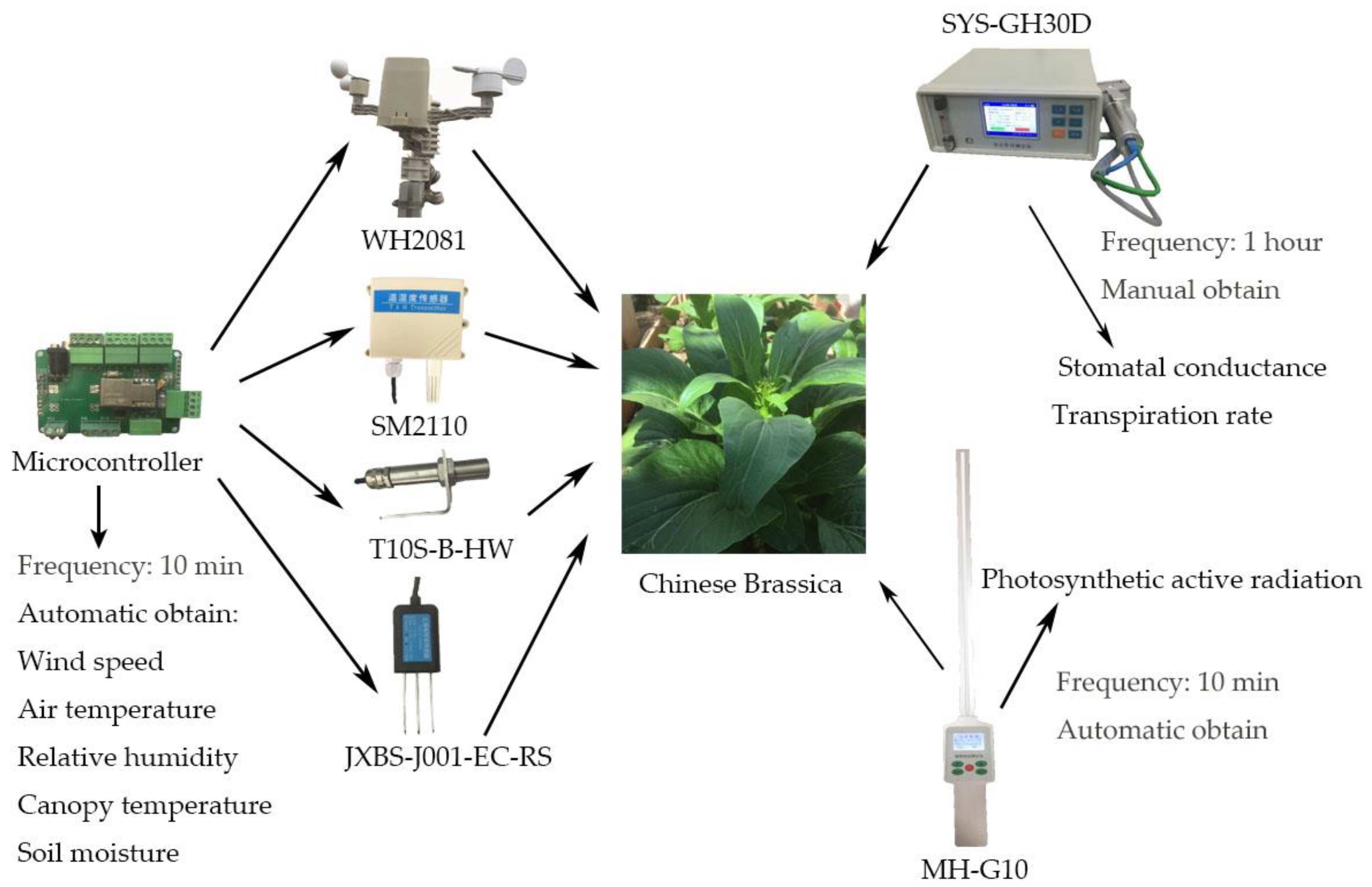
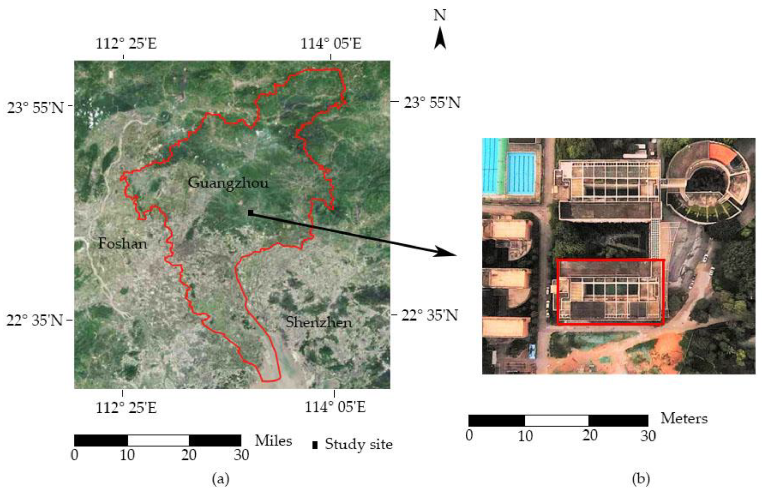
Traditional CWSI calculations are based on baseline canopy temperatures, which need to be measured multiple times to account for the variation in experimental conditions. Hence, simulating a baseline canopy temperature to simplify the measurements and experimental design would enhance the practicality of the CWSI. Thus, the specific objective of our study was to use an RF model to simulate the lower and upper baseline canopy temperatures for Chinese Brassica and to evaluate the accuracy of the predicted canopy temperatures.

In Section 2, the description of the field experiments and data used are given. Additionally, details of the RF model and evaluation criterion are given. This is followed by results and a discussion of the modeling of the lower and upper baseline canopy temperatures using the RF model in Section 3 and Section 4. Finally, the conclusion of the study is presented in Section 5.

2. Materials and Methods

2.1. Site Description and Experimental Design

This research was carried out twice at a trial site located at South China Agricultural University in Guangzhou (23°15′ L.N; 113°15′ L.E; Figure 1). The first (E1) and second experiment (E2) were conducted from 27 November to 31 December 2020, and from 25 May to 20 June 2021, respectively. The two experiments shared the identical experiment conditions, except at trial time. The area has a typical subtropical monsoon climate, and the average precipitation of E1 and E2 were 18 mm and 80 mm during the experimental period. The soil in the experimental station was sandy loam (sand = 58%, silt = 27% and clay = 15%). Chinese Brassica seeds were sown and regulated throughout the growing day using approaches including irrigation with adequate water, fertilization, and pest control. The fertilizer containing nitrogen, phosphorus, and potassium was supplemented at 10 day intervals. Twenty-day-old Chinese Brassica plants, each with four leaves and one core, were transplanted to flowerpots of the same size (0.15 m height and 0.22 m width) and with identical soil quality before the trial. The experiment ended when the bolt height of each Chinese Brassica plant was equal to that of the adjacent leaves. The experiment included six groups based on the field capacity (FC). Calculation of the field capacity was performed as follows [24]:

$$W=\left(\frac{m}{M}-1\right)\times 100\%,$$

(1)

where W represents the field capacity of the flowerpot, $m$ represents the soil moisture weight after irrigation with a sufficient amount of water for longer than 24 h, and $M$ represents the dry weight of the soil using the hot wind drying method (105 °C for 6 h).

In previous research, the water treatment group (i.e., Agam et al. [31], King et al. [37], Park et al. [22], and Bian et al. [24]) was usually split into three or four, in which one group with upper soil moisture represented the non-stressed condition, one group with lower soil moisture represented the severe stressed condition, and the remaining group represented a mild stressed condition. The crops’ response to soil conditions were different, and it is necessary to design more groups to test the crop response to different soil moisture levels that eventually affect the change in the CWSI. Furthermore, according to O’Shaughnessy et al. [47] and Osroosh et al. [48], the irrigation rule is effective based on the CWSI-TT method, where the CWSI is greater than a specific value in accumulated time. Therefore, six groups were designed in our study to determine the specific value of the CWSI in relation to trigger irrigation. Additionally, the stomatal conductance and transpiration rate were introduced to find the discrepancy within these groups. When the stomatal conductance or transpiration rate between any two groups is significantly distinct, the CWSI values between these two groups are helpful in finding a further threshold value [35].

In this study, each group has two Chinese Brassica plants, and the details of the groups are given in

Table 1. Descriptions of group based on treatment.

Group	Moisture Content	Treatment	Plants
T1	Near FC	Sufficient	Each group has two Chinese Brassica
T2	Near 85% of FC	Control
T3	Near 70% of FC	Control
T4	Near 55% of FC	Control
T5	Near 40% of FC	Control
T6	Deficit	No supplement

. A group denotes a specific water treatment. Plants subjected to Group T1 were supplied with sufficient water to keep the moisture content near the FC in order to estimate the lower baseline temperature, whereas those in Group T6 were subjected to severe stress by giving them no supplemental water. The data from Group T6 were used to obtain the upper baseline temperature. Groups T2, T3, T4, and T5 represented 85%, 70%, 55%, and 40% of the FC, respectively. The water was supplemented every day after measurement. The irrigation volume of Groups T1–T5 were 500 mL, 400 mL, 300 mL, 200 mL and 100 mL, respectively. The soil moisture was monitored daily using a soil moisture sensor (JXBS-J001-EC-RS, JINGXUN, China), which recorded the soil moisture at depths from 0 to 0.1 m at 10 min intervals.

2.2. Data Collection

The daily stomatal conductance (Sc) and transpiration rate (Tr) were monitored daily with a photosynthetic determinator (SYS-GH30D, SAIYA, China) by measuring fully expanded sunlit leaves from each group. The measurement range was 0~3000 μmol·m⁻²·s⁻¹ with an accuracy level of 3 μmol·m⁻²·s⁻¹. The average of five tested and two duplicated values was recorded as the measurement value for a group. The photosynthetic active radiation (Par) (MH-G10, LVBO, China) at a height of 0.2 m was measured at a 1 min interval and record ed as 10 min averaged values.

An online infrared radiometer (T10S-B-HW, MIAOGUAN, China) with a response time of less than 1 s, operating within an atmospheric window of 8~14 μm, was installed in each investigated group at a height of 0.3 m above the recent fully expanded sunlit leaves to measure the canopy temperature of the Chinese Brassica plants in that group. The measurement of multiple leaves for one plant was introduced to minimize the influence of two plants in a group. The radiometer was pointed at an angle of 45° toward the sunlit leaves, and the canopy temperature was recorded at 10 min intervals under clear sky conditions for canopy temperature was not change abruptly [37]. The installation of the radiometer was to ensure that the sunlight was completely on the leaves. The air temperature (Ta), relative humidity (RH) (SM2110, SONBEST, China) at a height of 1 m, and wind speed (WS) (WH2081, MISOL, China) at a height of 2 m were measured adjacent to the experimental zone. Every measurement was not at the same height to eliminate interference within the instruments. The canopy temperature, Ta, RH, and soil moisture were obtained using a microcontroller.

All climatic data were collected between 11:00 and 15:00 during the trial because the midday CWSI is more indicative of water status [17], and the components of the data collection system are shown in Figure 2. The meteorological conditions present during the trial are detailed in

Table 2. Maximum (max), minimum (min), mean, and standard derivation (Std) of the climatic values for E1 and E2.

Climatic Parameters	Max	Min	Mean	Std
Air temperature (℃)	34.80/43.48	16.50/26.90	25.75/37.08	3.68/3.38
Relative humidity (%)	59.7/90.56	11.20/36.25	38.22/57.76	7.81/10.79
Wind speed (km/h)	18.40/19.40	0.00/0.00	2.50/4.52	2.95/3.82
Photosynthetic active radiation (μmol·m−2·s−1)	2110.00/2867.00	0.00/2.00	641.00/1025.82	531.14/665.02

.

2.3. CWSI Calculation

The CWSI was calculated as follows [10]:

$$CWSI=\frac{T_c-T_{wet}}{T_{dry}-T_{wet}},$$

(2)

where $T_C$ (°C) represents the canopy temperature, $T_{wet}$ (°C) is the lower baseline of the canopy temperature, and $T_{dry}$ (°C) is the upper baseline of the canopy temperature.

The values obtained from Group T1 were considered to represent the lower baseline temperature ($T_{wet}$), whereas measurements from Group T6 represented the upper baseline temperature ($T_{dry}$). The values obtained for Groups T1 and T6 were used for modeling and evaluation. The CWSI values related to Groups T1 and T6 were not considered in the calculation. The $T_C$ values represented the actual measured values from Groups T2–T5, which were recorded at 10 min intervals. The CWSI values of Groups T2–T5 collected between 11:00 and 15:00 were used to calculate the daily CWSI.

2.4. RF Model

The RF model was first proposed in 2001 and is used for classification and prediction [49]. In our study, the RF model was used to simulate the lower and upper baseline canopy temperature using climatic parameters. It performs better than multiple linear regression, with a higher correlation of determination and a lower root mean squared error and mean absolute error, which are usually used to evaluate the performance of the model [50]. The structure constitutes a number of decision trees which are easy to establish and that share a similar simulating performance compared with neural networks [29,51], which are based on a feed-forward back-propagation network architecture, more complex than the decision tree. Generally, the process of building the RF model consists of sampling with replacement, establishing a decision tree with a certain quantity of samples, and integrating the outputs of each tree. The flowchart of the training model is presented in Figure 3.

In this study, the flowchart of the training model was as follows. Given an ensemble of dataset $n$, $D=\left\{\left(x_1,y_1\right),\dots ,\left(x_n,y_n\right)\right\}$, where $x_i$ ($i$ = 1, 2, …, n) is a vector of the descriptors and $y_i$ is the correspondingly targeted value, a portion of the dataset was randomly selected to form subset $m$ and construct $m$ trees. The targeted data in our study are $T_{wet}$ and $T_{dry}$, and the descriptors are Ta, RH, WS, and Par. Each subset was split into two sections using the corresponding values of specific features of the descriptors, and the total squared deviation of the targeted values was computed. The calculation used was as follows:

$$d=\underset{j,s}{\min }\left[\underset{c1}{\min }\sum _{x_i\in d_1\left(j,s\right)}{\left(y_i-c_1\right)}^2+\underset{c2}{\min }{\sum }_{x_i\in d_2\left(j,s\right)}{\left(y_i-c_2\right)}^2\right],$$

(3)

where $d$ represents the square deviation, $j$ represents a feature, $s$ represents the value corresponding to that feature, $d_1$ and $d_2$ represent two zones spilt by $s$, and $c_1$ and $c_2$ represent the average values of $y_i$.

When $d$ was at its minimum value among all calculations, the subset was segmented into two subtrees, named the left tree and the right tree. The above step was repeated until the trees were fully grown. Consequently, the outputs of all trees were integrated, with the final prediction made after each tree was finished, such that the number of splitting nodes was equal to the given value. This was usually equal to the average output.

It is noteworthy that the number of decision trees and the number of splitting nodes within each tree are vital parameters influencing the performance of the RF model. In general, having fewer decision trees or fewer splitting nodes could lead to underfitting [52], whereas having more could give rise to overfitting [53]. Thus, it is necessary to validate the model with different numbers of decision trees and splitting nodes.

When sampling with the replacement method is performed, parts of the sample may be repeatedly extracted, whereas others may never be selected. The left-out samples are called out-of-bag (OOB) samples. Feature importance is a useful way to evaluate the significance of each feature during model construction using OOB samples [54]. After adding man-made values to OOB samples to constitute a new dataset, the model was tested using an independent dataset. Generally, an evident decrease in the R² value demonstrates a high level of importance compared with the dataset without artificial values. The calculation used was as follows:

$$I=\frac{1}{n}{\sum }_{i=1}^n[{\left({\tilde{y}}_i-y_i\right)}^2-{\left(\dot{y_i}-y_i\right)}^2],$$

(4)

where $I$ represents the feature importance, $i$ represents the number of trees, ${\tilde{y}}_i$ represents the predicted value using man-made values, $y_i$ represents the targeted values in OOB samples, and $\dot{y_i}$ represents the predicted value using OOB data.

The Ta (SM2110, automatically obtained using a microcontroller), RH (SM2110, automatically obtained using a microcontroller), WS (WH2081, automatically obtained using a microcontroller), and Par (MH-G10, automatically obtained) data collected during the crop period from May 25 to June 20 and recorded as 10 min values were used for model development and validation, and the outcomes were $T_{wet}$ and $T_{dry}$ (T10S-B-HW, automatically obtained using a microcontroller). Python was used to build and validate the RF model. Initially, the data used for model development were standardized and randomly split into training (development, 70%) and testing (validation, 30%) datasets.

2.5. Statistical Analysis

In this study, graphical, linear regression, and variance analyses were conducted to assess the correlations between the canopy temperature and the climatic parameters, the effect of the RF model in forecasting $T_{wet}$ and $T_{dry}$, and the linear correlations of the CWSI with Sc and Tr. The discrepancy of the CWSI within the Groups T2–T5 was evaluated using ANOVA (p ≤ 0.05); with the hypothesis, there were no significant differences within the Groups T2–T5. The presence of a significant difference ($p$ ≤ 0.05) in the regression line slope was evaluated using t-tests. The mean absolute error (MAE), root-mean-square error (RMSE) and coefficient of determination (R²) used in this study were calculated as follows:

$$MAE=\frac{1}{n}{\displaystyle \sum }\left|\widehat{y}-y\right|,$$

(5)

$$RMSE=\sqrt{\frac{\sum {\left(\widehat{y}-y\right)}^2}{n}},$$

(6)

$$R^2={\left[\frac{n\sum y\times \widehat{y}-\sum y\sum \widehat{y}}{\sqrt{\left[n\sum y^2-{\left(\sum y\right)}^2\right]\left[n\sum {\widehat{y}}^2-{\left(\sum \widehat{y}\right)}^2\right]}}\right]}^2,$$

(7)

where $y$ represents the measured value, $\widehat{y}$ represents the model’s predicted value, and $n$ is the number of samples.

3. Results

3.1. Environmental Parameters and Canopy Temperature Characteristics

The histogram for environmental parameters (Ta, RH, WS, Par) measured between 11:00 and 15:00 from 27 November to 31 December 2020, and 25 May to 20 June 2021, is shown in Figure 4. There were some differences between E1 and E2. At least 70% or more of Ta and RH in E1 were ≤30 °C and ≤40%, respectively, whereas those in E2 were ≥35 °C and ≥50%. WS and Par showed a similar range in both E1 and E2, in which the majority of WS and Par in E1 were lower than those of E2. The climate was clearly hot and wet and there were high Ta, RH, and Par values in E2, but the climate was cool and dry in E1. The large range of ambient climatic characteristics was beneficial for RF model construction, as it extended the dataset and enhanced the prediction performance under more variable conditions.

The canopy temperatures in Groups T1 ($T_{wet}$) and T6 ($T_{dry}$) (shown in Figure 5) also fluctuated evidently. The max differences between $T_{wet}$ and $T_{dry}$ in E1 and E2 were 6 and 20 °C, respectively. This distinction is mainly caused by the higher Ta and Par in E2 for the greater response of stressed crops to the environment [31]. The maximum of $T_{wet}$ in E1 was ≤30 °C, whereas the minimum of $T_{wet}$ in E2 was ≥30 °C. Serval $T_{dry}$ values in E1 were ≥30 °C, but the bulk of these values in E2 were ≥30 °C. Furthermore, it was notable that the daily $T_{dry}$ after 15 June increased abruptly, presumably due to the invisible damage associated with the occurrence of a soil water deficiency over a long period of time, which led to its being highly sensitive to Ta and Par. Generally, the averaged values of $T_{dry}$ exceeded that of $T_{wet}$ in both E1 and E2.

To facilitate an understanding of the relationship between environmental parameters and the canopy temperature of Chinese Brassica, a correlation coefficient matrix map is presented in Figure 6. Values below zero represent negative correlations, whereas values above zero represent positive correlations; the color shade represents the inordinate influence, lighter means highly positive and darker means strongly negative. $T_{wet}$ and $T_{dry}$ had different degrees of positive correlation with Ta, Par, and WS, among which the correlation coefficient of over 0.84 between Ta and the canopy temperature ($T_{wet}$ and $T_{dry}$) was extremely significant. The difference in correlation coefficients between $T_{wet}$ and $T_{dry}$ was slightly related to Ta, whereas the differences in relation to RH and WS were 0.12 and 0.16, respectively, indicating relatively distinct discrepancies. In contrast to Ta, Par and WS, RH had a negative correlation of over 0.5 with the canopy temperature. Thus, the actual effects of the climatic characteristics on $T_{wet}$ and $T_{dry}$ were not necessarily equal.

To evaluate the distribution of canopy temperature and the difference between two Chinese Brassica plants, the ANOVA analysis was conducted and presented in

Table 3. The result of the test for Gaussian distribution of two plants in each group.

Group	Plant	Chi-Square	Degrees of Freedom	Significance
T1	1	105.721	114	0.698
	2	96.419	126	0.977
T6	1	82.775	156	1.000
	2	59.209	154	1.000

and

Table 4. The result of the test for independence of two plants in each group.

Group		Sum of Square	df	Mean Square	F Value	Sig.
T1	Between groups	0.049	1	0.049	0.004	0.950
	Within groups	6545.713	514	12.735
	Total	6545.762
T6	Between groups	0.119	1	0.119	0.003	0.956
	Within groups	20,321.626	514	39.536
	Total	20,321.746

. According to Table 3, both plant 1 and plant 2 in Group T1 submitted to Gaussian distribution with the chi-squared test and were lower than the critical values under the significant level of 0.05. The similar results were also found in group T2. Simulating the canopy temperature performs well with the Gaussian distribution to eliminate the skewness when the samples are randomly divided. Considering the small number of plants in Groups T1 and T6, it is necessary to test the difference in canopy temperature within two plants. According to Table 4, the significance in Groups T1 and T6 was distinctly over 0.05, demonstrating the high correlation between plant 1 and plant 2. Therefore, using the mean value of two plants to represent the measured value of the Groups was viable.

3.2. Estimation of the Lower Baseline and Upper Baseline of Canopy Temperature

To attain the best simulation performance, the RF model was developed using a large number of scenarios to select the optimal parameterization. Some essential parameters, such as the number of decision trees and the number of splitting nodes in each tree, were evaluated using the R², RMSE, and MAE, as shown in Figure 7. In the process of increasing the number of decision trees, the R² values for $T_{wet}$ and $T_{dry}$ were 0.52 and 0.49 at the beginning of the simulations and remained stable at 0.83 and 0.81 when the number of decision trees exceeded 50. The RMSE and MAE decreased to 1.54 and 1.11 for $T_{wet}$, and to 2.64 and 2.01 for $T_{dry}$ with the increasing number of decision trees and splitting nodes. The R² values after one split were significantly lower when modeling both $T_{wet}$ and $T_{dry}$, but splitting many nodes did not obtain the highest R² value—this was obtained with six nodes. It was concluded that models with many decision trees and splitting nodes do not perform better than those with suitable numbers. In addition, the changing number of splitting nodes contributes an abrupt change toward optimal R², RMSE, and MAE values. According to the validation test, the best performing model for the prediction of $T_{wet}$ and $T_{dry}$ was a model with 100 decision trees and six splitting nodes.

The feature importance of Ta, RH, WS, and Par is presented in Figure 8. The proportions to which Ta, RH, WS, and Par contributed to the simulation of $T_{wet}$ were 65.9%, 2.9%, 2.1%, and 29.1%, respectively. However, the ratios of Ta, RH, and WS used for simulating $T_{dry}$ slightly increased by 4%, 4%, and 1%, respectively, and that of Par decreased by 9%. Ta occupied a proportion of over 60%, indicating its dominant contribution to the modeling process. The ANOVA results for predicting $T_{wet}$ and $T_{dry}$ are shown in

Table 5. The ANOVA results for predicting $T_{wet}$ and $T_{dry}$.

Target	Model	Sum of Squares	df	Mean Square	F Value	Sig.
$T_{wet}$	regression	1045.338	4	261.335	35.682	<0.0001
	residual	3830.475	523	7.324
	total	4875.813	527
$T_{dry}$	regression	3562.789	4	890.697	35.862	<0.001
	residual	12,989.648	523	24.837
	total	16,552.437	527

. According to the table, the significances of the F value are <0.0001, implying a distinct difference from zero of the coefficients of regression both in $T_{wet}$ and $T_{dry}$. The sum of the square for the residual in is distinctly lower than that of $T_{dry}$, indicating the better performance for $T_{wet}$ compared with $T_{dry}$. Although RH and WS separately had good correlations with $T_{wet}$ and $T_{dry}$, both contributed poorly to the integrated regression. Nevertheless, all features were considered for model development due to the limited dataset.

The performance of the model was estimated using the scatter plots presented in Figure 9 and Figure 10, and the error analysis is presented in

Table 6. Descriptive error statistics of the RF model for predicting $T_{wet}$ and $T_{dry}$.

Target	Experiment	Model	R2	RMSE	MAE
$T_{wet}$	E1	development	0.90 *	0.96	0.76
		validation	0.80 *	1.62	1.25
	E2	development	0.91 *	0.97	0.83
		validation	0.83 *	1.41	1.11
$T_{dry}$	E1	development	0.88 *	1.33	1.03
		validation	0.77 *	2.01	2.00
	E2	development	0.89 *	1.65	1.45
		validation	0.80 *	2.27	2.09

* represent the significance at the 0.05 probability level as indicated by t-test.

. The linear equation of the predicted RF model versus the measured values resulted in R² values of 0.90 and 0.80 for development and validation in E1, and of 0.91 and 0.83 for development and validation in E2. The RMSE values of the RF model for development and validation were 0.96 and 1.62 °C in E1, and were 0.97 and 1.41 °C in E2, respectively. The MAE values for development and validation were 0.76 and 1.25 °C in E1 and were 0.83 and 1.11 °C in E2, respectively. The higher R² and lower RMSE and MAE for validation in E2 denoted a slightly better performance compared with E1. The linear equation of the predicted RF model versus the measured $T_{wet}$ values resulted in R² values of 0.88 and 0.77 for development and validation in E1 and value of 0.89 and 0.80 for development and validation in E2. The RMSE values for development and validation were 1.33 and 2.01 °C in E1 and were 0.65 and 1.2.27 °C in E2, respectively. The MAE values for development and validation were 1.03 and 2.00 °C in E1 and were 1.45 and 2.09 °C in E2, respectively. The model validation in E2 performed well in terms of R², but poorly in terms of RMSE and MAE, compared with E1.

Linear correlations between the measured and predicted $T_{wet}$ and $T_{dry}$ values were significant ($p$ < 0.05) for the eight models. Moreover, the slopes of the regression lines were significantly different ($p$ < 0.05) from 0. The high correlation of determination between the measured values and predicted values both in E1 and E2 implied an insignificant difference between measurements and predictions. It also demonstrated that the RF model can simulate the lower and upper baseline canopy temperature well. The scatter plots also indicate that the RF model performed poorly with high temperature values. Overall, E1 and E2 shared similarly good results in predicting $T_{wet}$ and $T_{dry}$.

The variation in the prediction error for $T_{wet}$ and $T_{dry}$ is presented in Figure 11. The error was taken as the predicted value minus the measured value. The mean values of the prediction error for $T_{wet}$ and $T_{dry}$ were 0.07 and 0.10 °C for development and 0.18 and 0.22 °C for validation in E1, whereas they were 0.05 and 0.09 °C for development and 0.11 and 0.21 °C for validation in E2. The average prediction error values for the eight models were greater than zero, displaying a positive bias between measurement and prediction. It was observed that the error variance of $T_{wet}$ was less than that of $T_{dry}$ for both models in E1 and E2. There was little difference in bias between E1 and E2 for $T_{wet}$ and $T_{dry}$. Furthermore, the range of prediction errors for validation was slightly wider than that for development, resulting in a larger RMSE value. In conclusion, the results show that the accuracy of estimating $T_{wet}$ was better than that of $T_{dry}$ for both models in E1 and E2.

3.3. CWSI Characteristics

Daily CWSI values determined using measured and predicted $T_{wet}$ and $T_{dry}$ values were calculated for different water Groups (T2–T5) and are shown in Figure 12. The four treatment groups showed similar changes. The CWSI values determined using measured $T_{wet}$ and $T_{dry}$ values increased from Group T2 to Group T5 on the whole. A host of T2 values were below 0.4, whereas the T3, T4, and T5 values transcended 0.2. The majority of CWSI values from T2–T5 had similar fluctuation ranges of 0.4, 0.3, 0.3, and 0.4, respectively. The maximum daily CWSI values based on predictions in the four treatment groups increased successively, giving results of 0.4, 0.5, 0.6, and 0.8, similar to the measured values. In total, CWSI values were significantly different within water treatment groups shown in

Table 7. The mean CWSI for different groups in two experiments.

Experiment	Group	CWSI
		Measured Values	Predicted Values
E1	T2	0.2111	0.2176
	T3	0.3439	0.3429
	T4	0.4815	0.4832
	T5	0.5360	0.5449
		<0.05 *	<0.05 *
E2	T2	0.2348	0.2521
	T3	0.3561	0.3631
	T4	0.4627	0.4656
	T5	0.5621	0.5765
		<0.05 *	<0.05 *

* Significant at the 0.05 probability level as indicated by Duncan’s multiple range test.

, whereas CWSI values based on measurements and predictions were not significant. It was concluded that the CWSI values within four groups were distinctly different either in E1 or E2. It also implied that the CWSI values based on predicted values, compared with the CWSI values using measured values, share a similar performance in indicating the response to soil moisture. In addition, the average predicted values for the four treatment groups were 0.01 and 0.03 greater than the measured values in E1 and E2, respectively. The majority of values for the four groups in E1 were lower than that of E2 due to the lower difference of $T_{wet}$ and $T_{dry}$ in E1.

3.4. CWSI and Stomatal Conductance and Transpiration Rate

The connection between the CWSI and the crop-based indicators associated with crop water stress, linear regression, and scatter plots of Sc versus the CWSI values determined using measured and predicted $T_{wet}$ and $T_{dry}$ is presented in Figure 13. The linear correlation between Sc and CWSI was significant ($p$ < 0.05), with R² values of 0.54 and 0.45 in E1 and of 0.61 and 0.60 in E2, respectively, indicating a negative relationship between the CWSI and Sc. The average Sc values of plants from Groups T2 and T3 were significantly different ($p$ < 0.05) from those in Groups T4 and T5, whereas the mean difference between T4 and T5 plants was not significant. According to the linear equation, the value of Sc in E1 and E2 were 0.0108 and 0.0111 μmol·m²·s⁻¹ based on the measured baseline under a well-watered status, whereas they were 0.0086 and 0.0117 μmol·m⁻²·s⁻¹ based on the predicted baseline. In addition, when the CWSI value exceeded 0.8, the values of Sc were near zero, indicating that the majority of stomata were closed.

The correlation between the Tr and the CWSI is also presented in Figure 14, implying that an inverse relationship similar to that shown for Sc was present, whereas the R² values of 0.32 and 0.25 in E1 and of 0.19 and 0.18 in E2 were evidently lower. In addition, the mean values of Tr for the four water treatment groups did not differ significantly. As is shown in the linear regression, when the CWSI values determined using measured and predicted $T_{wet}$ and $T_{dry}$ values approached zero, the values of Tr were 0.1275 μmol·m⁻²·s⁻¹ and 0.1304 μmol·m⁻² s⁻¹ in E2, respectively, and 0.1462 μmol·m⁻²·s⁻¹ and 0.1102 μmol·m⁻²·s⁻¹ in E1. However, when Chinese Brassica suffered from severe water stress and the CWSI value exceeded 0.8, the values of Tr were near zero, identical to the trend shown for Sc. Considering the high R² values, Sc was determined to be more suitable for assessing the application of the CWSI for Chinese Brassica than Tr [30]. In summary, the distinction between CWSI values determined using measured and predicted $T_{wet}$ and $T_{dry}$ values was not significant. It was also observed that the differences in Sc and Tr among the four water treatment groups were not distinct, especially between Groups T3 and T4. When the CWSI was approximately equal to 0.4, the values of Sc and Tr in Groups T2 and T5 could be easily distinguished.

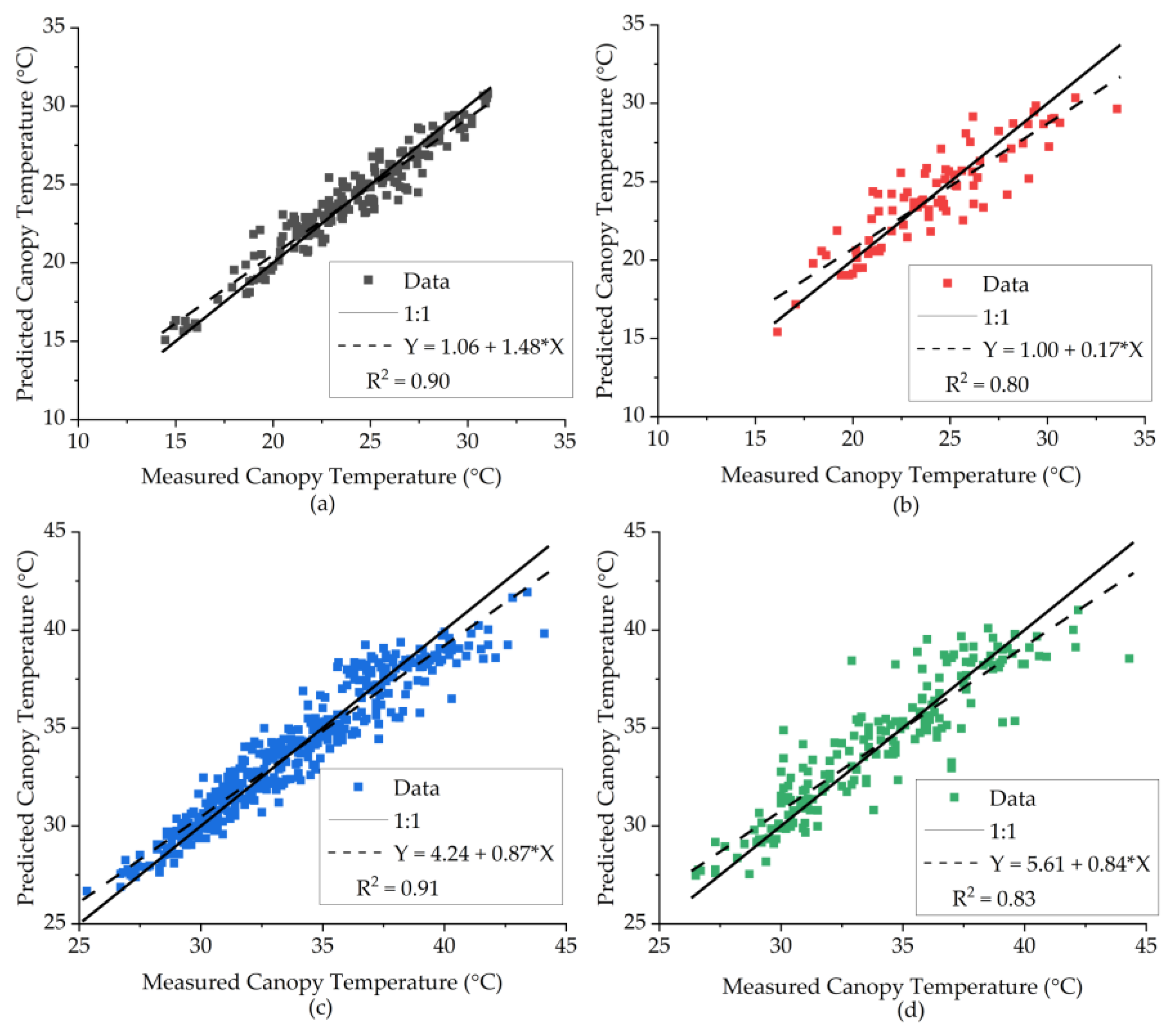
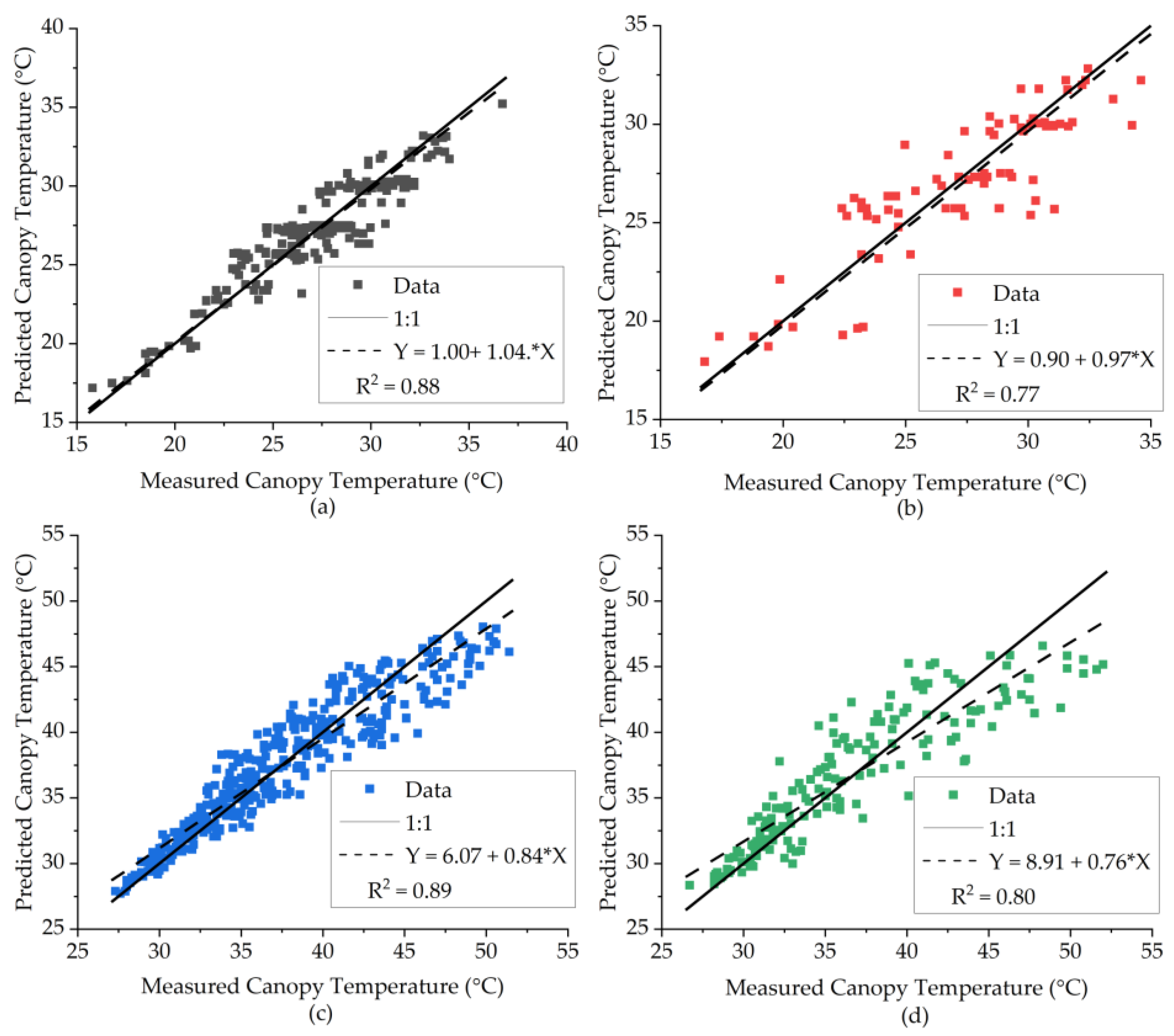
4. Discussion

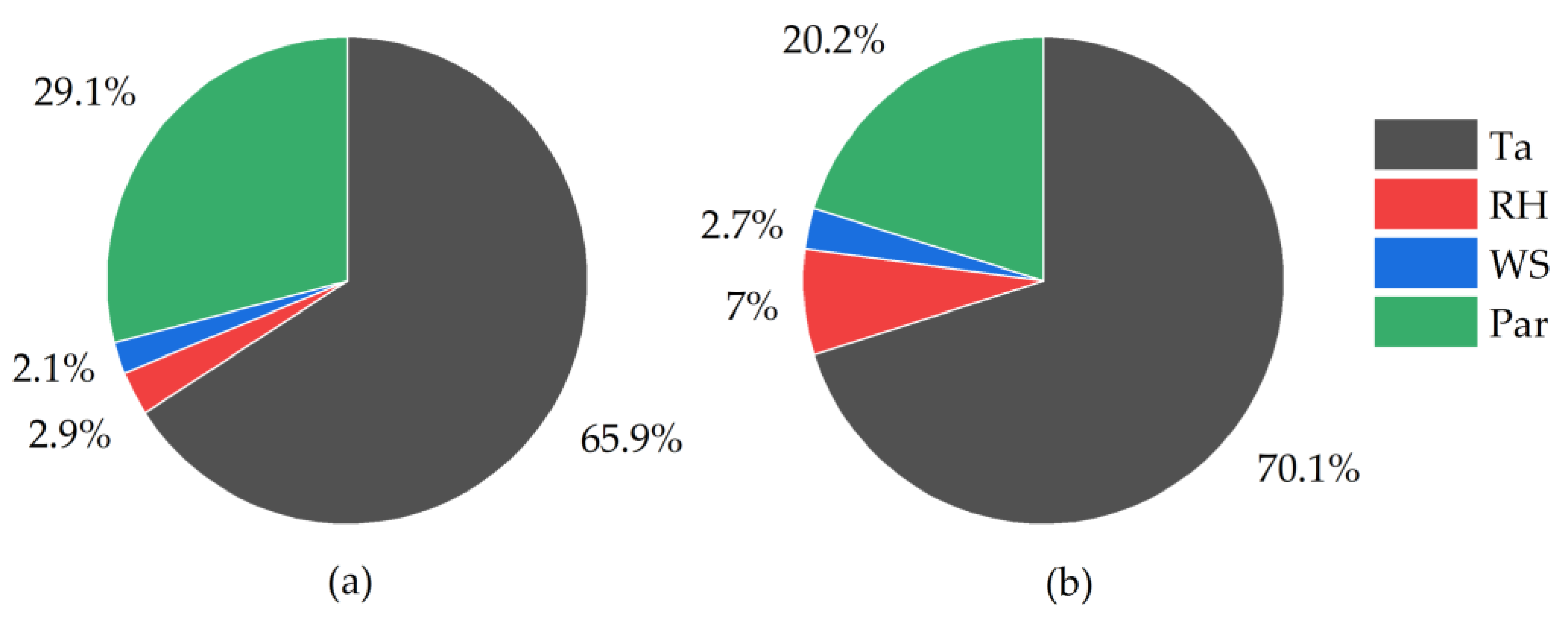
Frequently measuring and $T_{dry}$ restricts the practical application of the CWSI. In this study, an RF model using easily obtainable environmental parameters (Ta, RH, WS, and Par) exhibited viability for simulating $T_{wet}$ and $T_{dry}$ for Chinese Brassica. King et al. [28] were the first to predict $T_{wet}$ based on a neural network and demonstrated an excellent R² value of 0.88. This result is similar to that obtained for the model developed in our study. However, our study illustrated the potential to simulate $T_{dry}$ at the same time. Furthermore, our study used Par rather than net solar radiation [28,51], and Par made a greater contribution to model construction than WS and RH. Neukam et al. [50] developed an empirical regression model to predict winter wheat canopy temperature for three irrigation levels and the results showed R² values of 0.9. However, the RMSE values of 1.5~2.0 °C were higher than the RMSE in our study. Wang et al. [55] simulated the canopy temperature in a green house and evaluated the performance of multiple linear regression using air temperature, relative humidity, and solar radiation; they found an R² value of 0.87. However, the environment in their study was not sufficiently variable, as the temperature and radiation in the greenhouse were ≤37 °C and 500 W/m². Duan et al. [56] used the surface ground temperature and air temperature to predict the wheat canopy temperature, and the neural network model showed that the R² and RMSE value were 0.92 and 1.64, respectively. However, the tested samples were ≤50, lower than in our study.

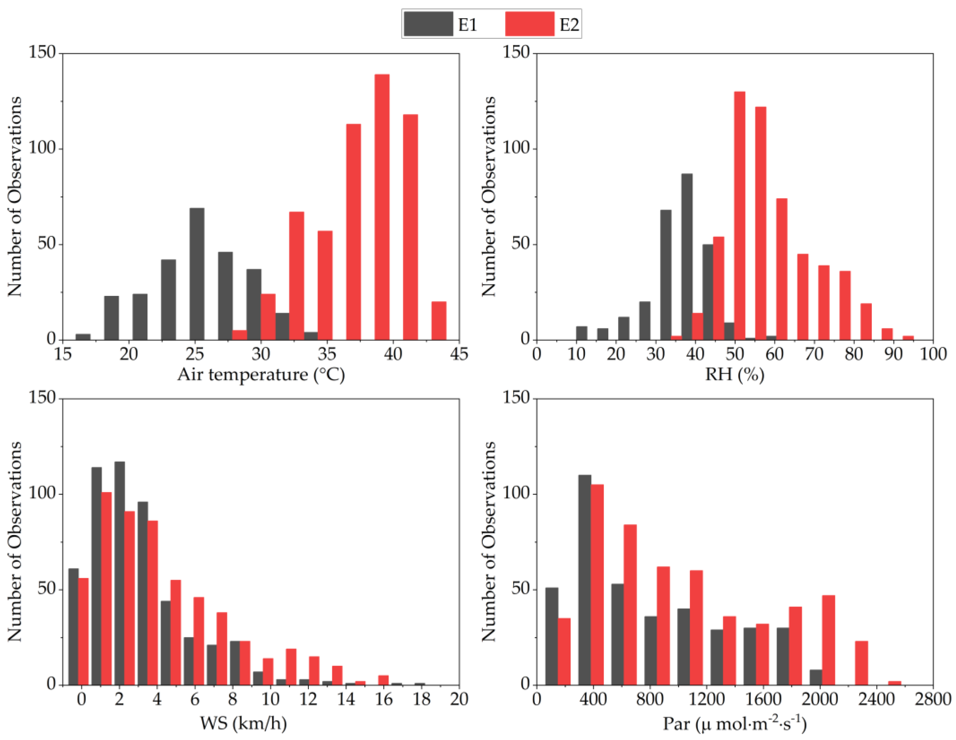
RF models are principally driven by data, indicating the importance of the original dataset having many precise samples. Site-specific data are easily obtained, but there are potential difficulties. For example, the instruments are stationary and may be damaged by pests and extreme weather. Moreover, its energy-consuming nature entails high equipment requirement [57]. The climatic characteristics used in this experiment, especially Par, were highly variable. However, the majority of values were relatively low, and the RF model performed better with lower values than with higher values. Nevertheless, our model could be optimized by adding corresponding data to minimize the level of skewness.

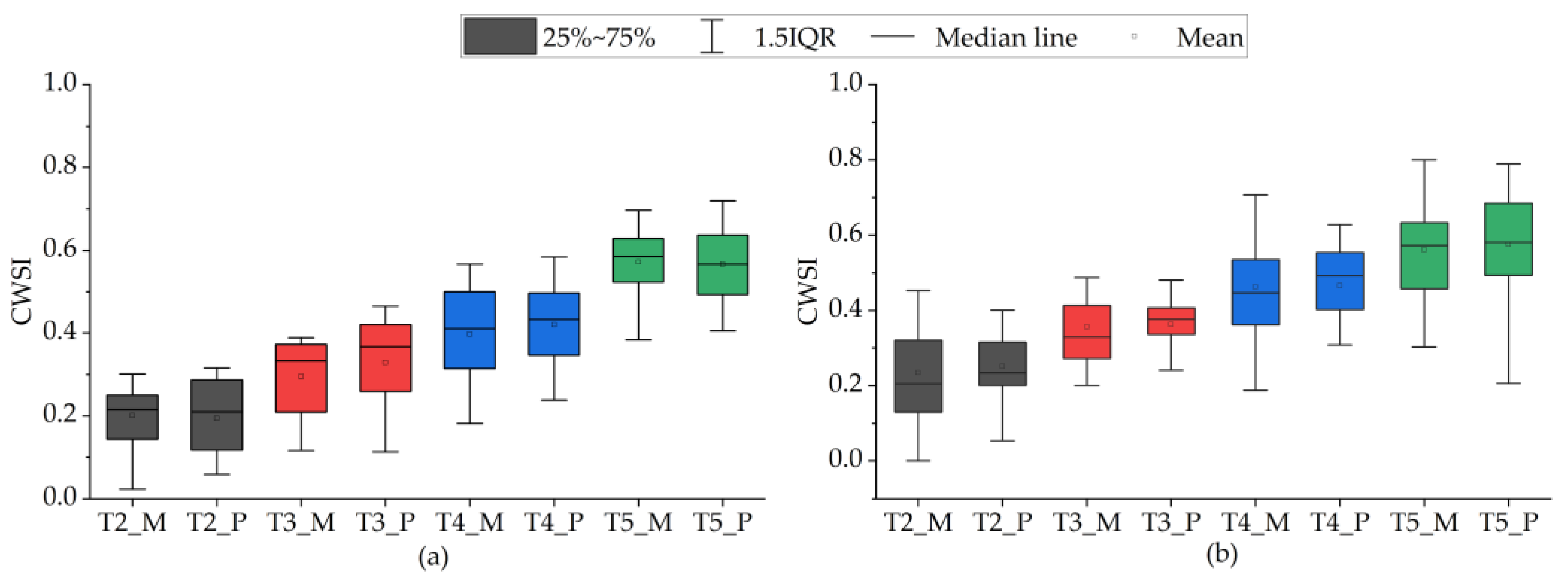
Overall, the study provides a feasible and reliable approach that can be used to determine the canopy temperature to calculate the CWSI and then make irrigation decisions. O’Shaughnessy et al. [47] provided the CWSI-TT method for scheduling irrigation, where the decision rule was such that the CWSI was greater than a threshold value of 0.45 in accumulated time; the result indicated the effective trigger of CWSI-TT for automatic irrigation. Osroosh et al. [48] used dynamic time and the CWSI as the threshold for irrigation and founded that a CWSI of 0.46 ± 0.11. 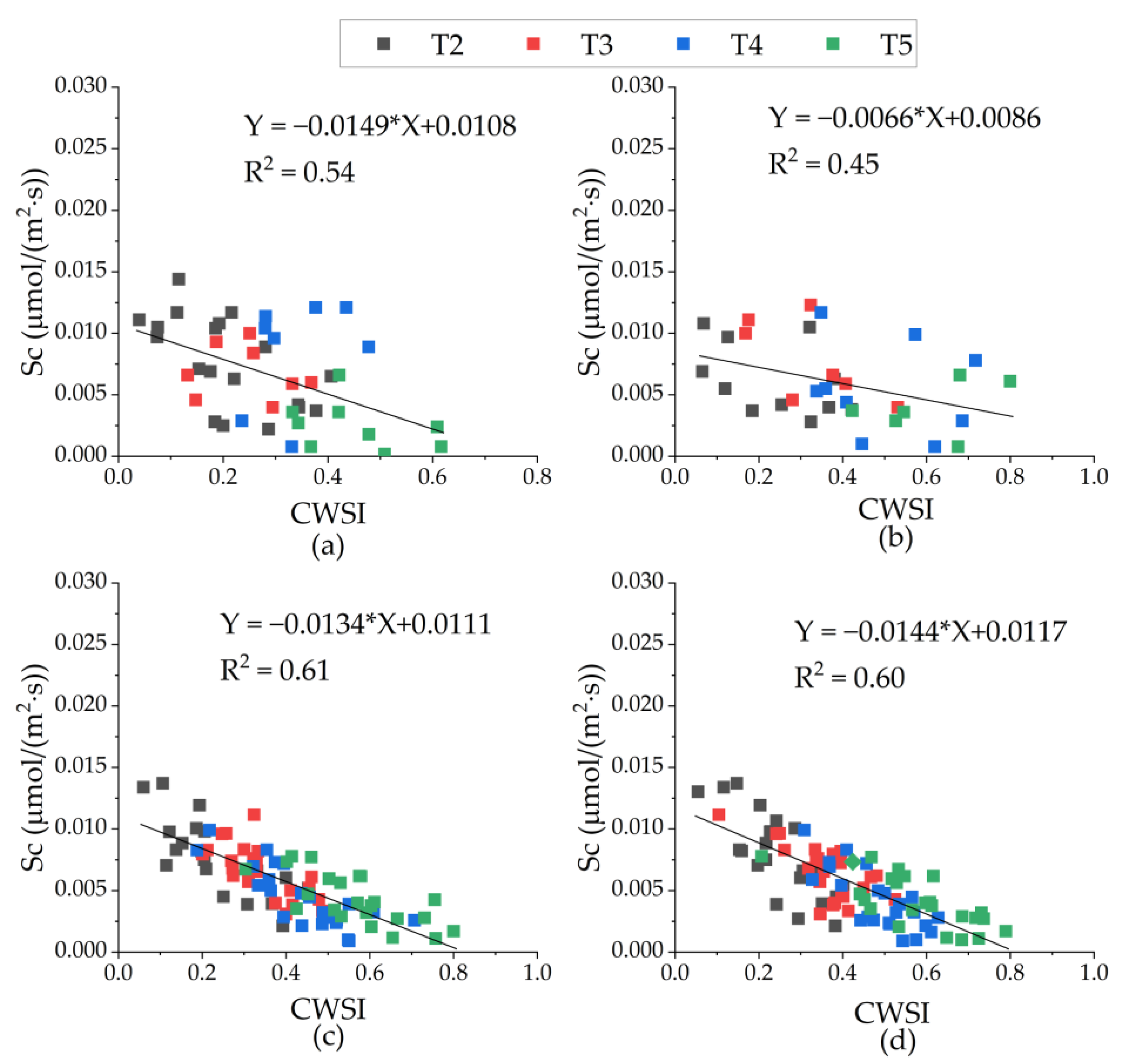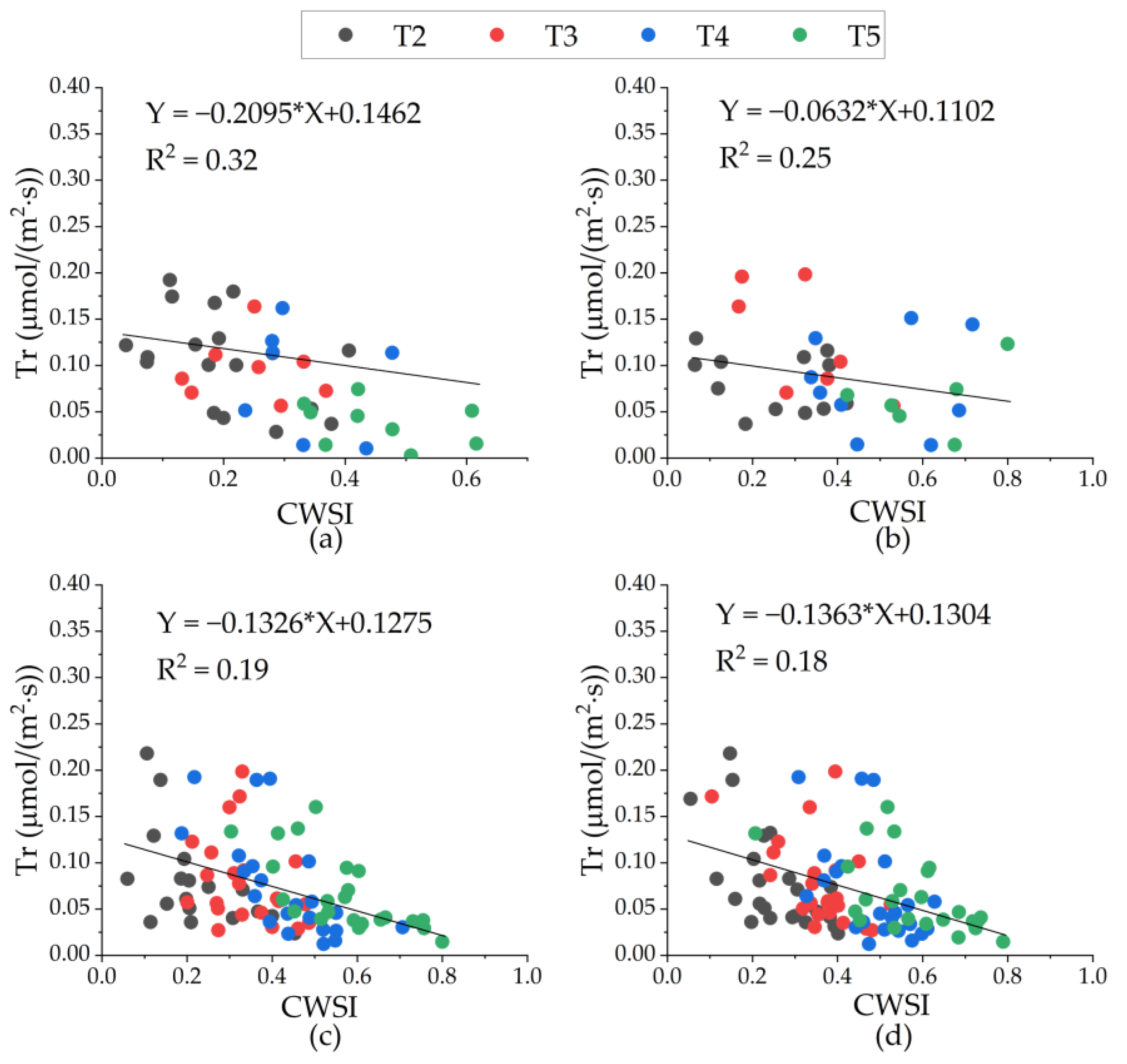According to Figure 13 and Figure 14, the Sc and Tr values between Groups T3 and T4 were distinct, whereas most CWSI values for Group T3 were ≤ 0.4 and those of Group T4 were ≥ 0.4, denoting a possibility of irrigation with a CWSI value of over 0.4. In further research, the CWSI-TT, where the CWSI is greater than 0.4 in accumulated time, could be used for irrigation in real time, which avoids over irrigation and enhances water efficiency.

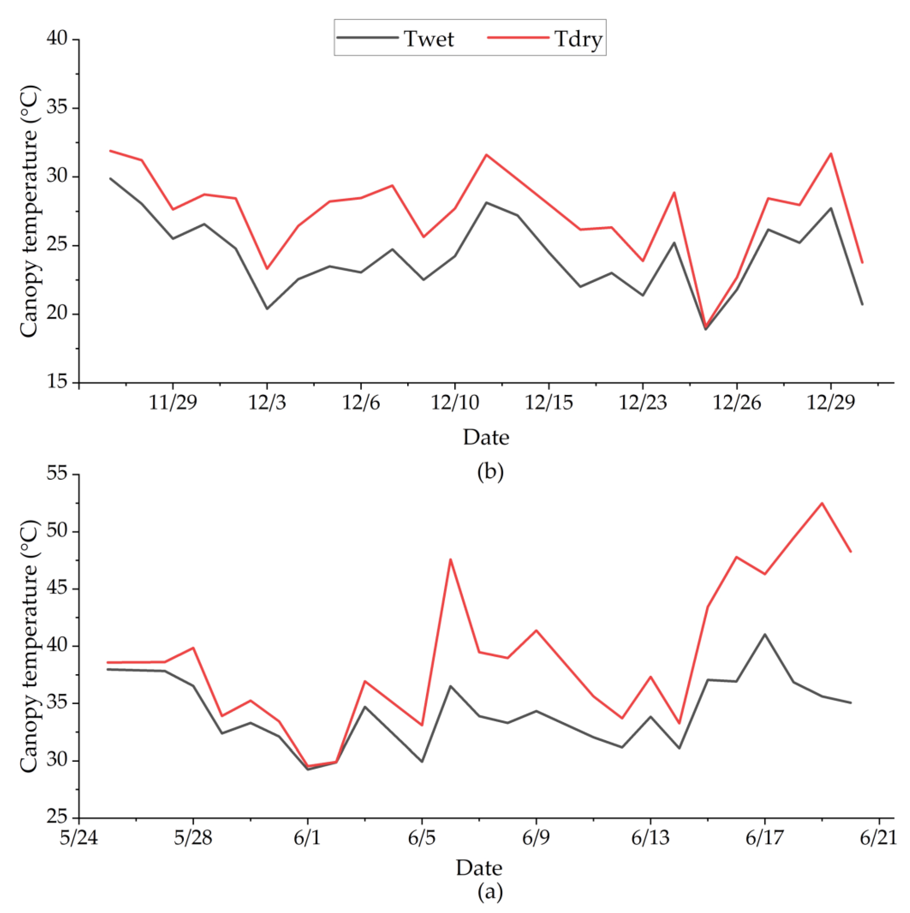
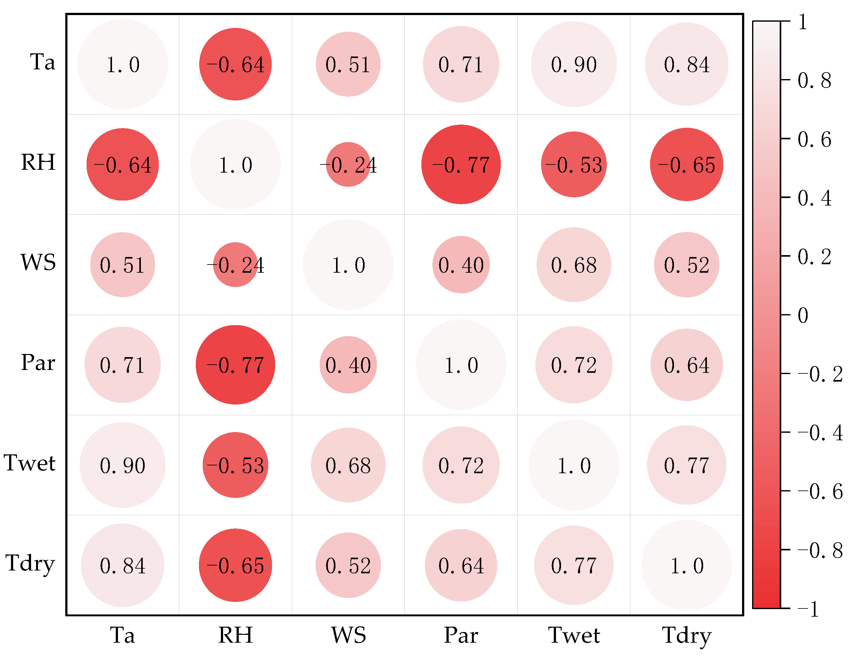
In addition, the study illustrates a good correlation of Par with $T_{wet}$ and $T_{dry}$ for Chinese Brassica, and this is relevant for modeling. Previous literature has indicated that the canopy temperature of stressed crops shows a greater response to high radiation than well-watered crops [31,39]. When the average daily Ta was ≧35 °C and the daily Par was ≧1000 μmol·m⁻²·s⁻¹, the difference between $T_{dry}$ and $T_{wet}$ abruptly increased, as shown in Figure 5, indicating a relationship between the canopy temperature and Par. In this study, the RF model developed using ambient environmental parameters (Ta, RH, WS, and Par) demonstrated the viability of estimating $T_{wet}$ and $T_{dry}$ with good results. Considering the slightly greater relationship between climatic parameters and $T_{wet}$ compared with $T_{dry}$, the prediction of $T_{wet}$ was better in terms of both model development and validation. Previous research has demonstrated similar performances using Ta plus a constant such as $T_{dry}$ [27,29,32]. However, the maximum differences between $T_{dry}$ and Ta for Chinese Brassica can be up to 10.0 °C, whereas the minimum is close to 1.0 °C. Therefore, utilizing air temperature plus a specific constant to replace $T_{dry}$ could increase or decrease the value of the CWSI, whereas forecasting $T_{dry}$ could relatively diminish the difference.

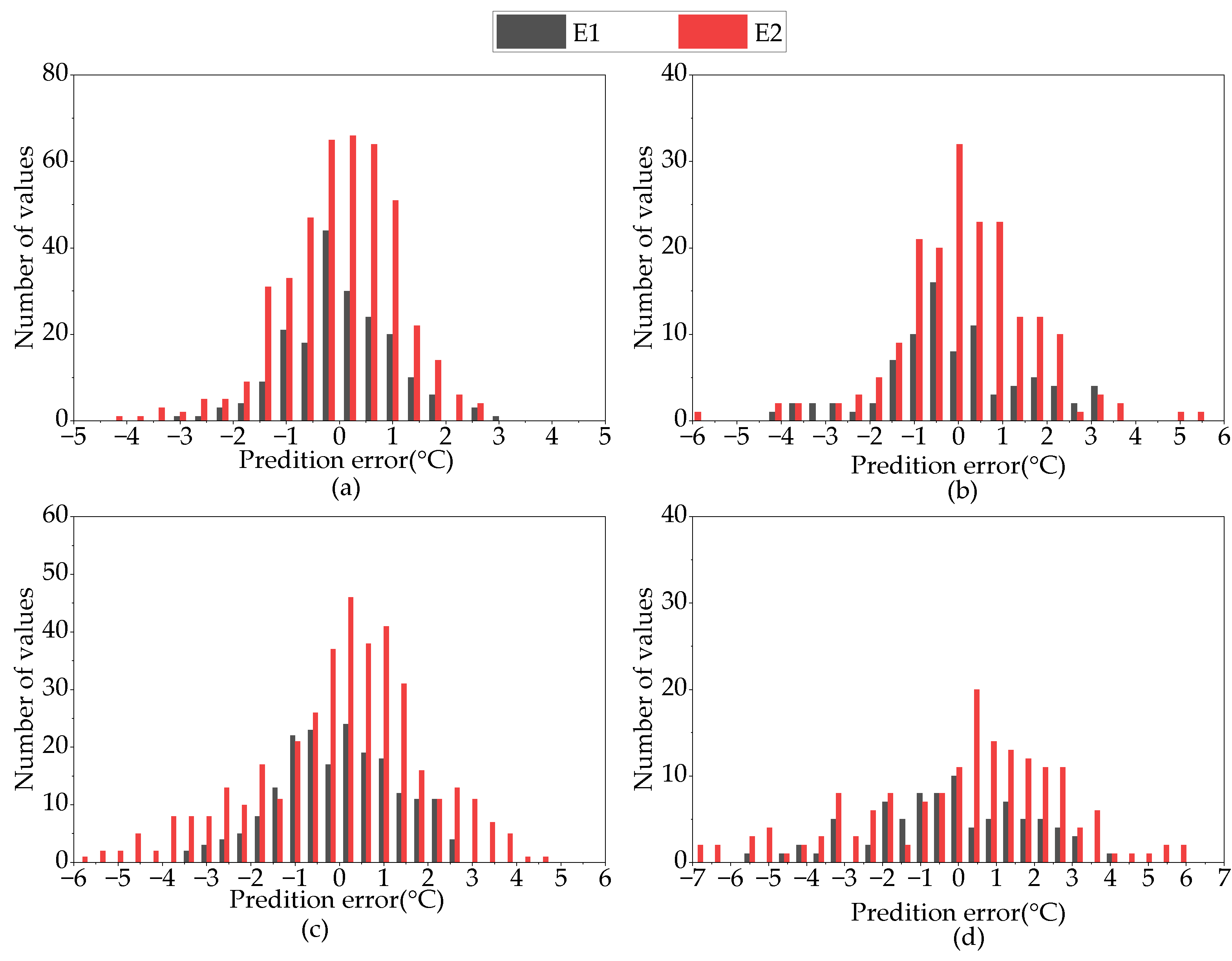
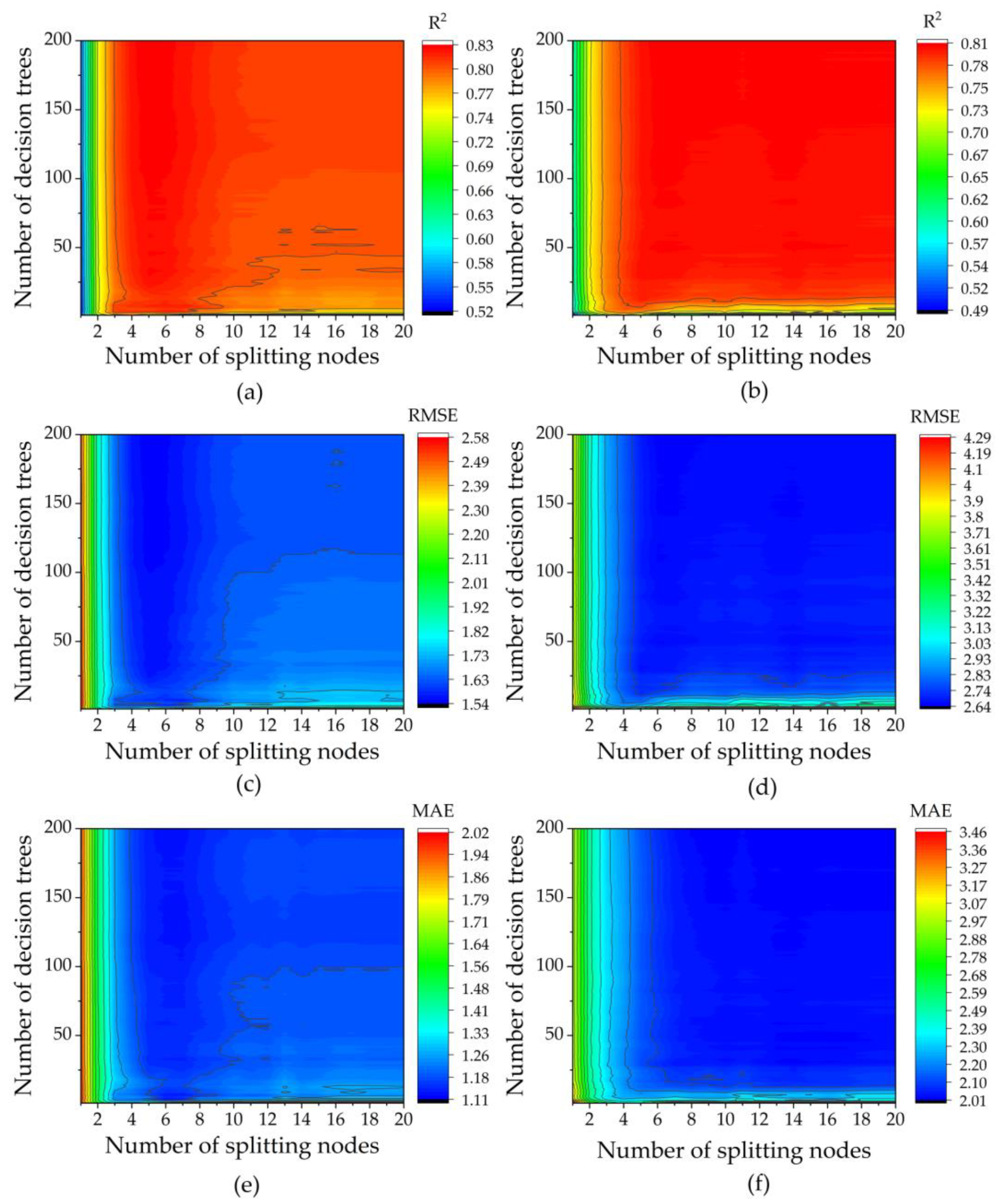
Generally, the CWSI values were negatively correlated with soil moisture values, implying that water paucity leads to high CWSI values. The daily CWSI values decreased to near or exactly zero, mainly due to the slight difference between $T_{dry}$ and $T_{wet}$ in response to lower Ta and Par values. Thus, the discrepancies in the CWSI values between the four water treatment groups were not significant. The multiple prediction errors for $T_{wet}$ were lower than for $T_{dry}$, as shown in Figure 9 and Figure 10, indicating higher values of $T_{dry}$ minus $T_{wet}$ based on predicted values. Thus, the average daily CWSI values determined using predicted $T_{dry}$ and $T_{wet}$ values slightly exceeded the measured values. The daily CWSI values based on the predicted values from the four water treatment groups had the characteristics of a narrow range and a slightly higher mean value compared with the measured values. In Table 5, the daily mean CWSI values for the four groups are compared, and the results show that the CWSI increases as the soil moisture decreases, similar to the present research of Irmak al. [32], Khorsandi et al. [34], and Jamshidi et al. [57]. The mean CWSI values within Groups T2–T5 were distinct with significance values < 0.05 either in E1 or E2.

According to Table 3 and Table 4, the significance of the F value for predicting $T_{wet}$ and $T_{dry}$ indicated a meaningful regression based on the RF model, whereas the high R² values in E1 and E2 were significant, implying an insignificant difference between measured values and predicted values. In addition, two plants in each group were lower in two experiments, but the measurement of multiple leaves from one plant was introduced to minimize the influence as much as possible, and this possibly affected the correlation between the CWSI and Sc and Tr.

Under soil water stress conditions, the stomatal closure further increases the canopy temperature and decrease the transpiration [58]. The relationship between the daily CWSI and Sc was stronger than Tr. This is because the fluctuated range of Sc in Chinese Brassica was 0~0.015 μmol·m⁻²·s⁻¹, lower than Tr (0~0.20 μmol·m⁻²·s⁻¹), and the Sc was more sensitive to the soil moisture [14]. The transpiration in Chinese Brassica, compared with the CWSI, does not change abruptly with the stomatal closure [5], implying the retardation of variation in Tr that eventually influenced the correlation between Tr and the CWSI. Additional details have been presented by Ben et al. [59] and Agam et al. [31]. They mentioned the potential effect of clouds and low radiation on transpiration. The daily Sc variance between T3 and T4 was distinct, whereas there was no significant difference between T4 and T5. Many CWSI values in T4 and T5 were over 0.4. From the producer’s perspective, Chinese Brassica might suffer from water stress when the CWSI value exceeds 0.4, and the level of scheduled irrigation is also considerable. The correlation between the CWSI and irrigation volume could be analyzed in a future study to achieve precise water control.

Our study focuses on simulating the canopy temperature of Chinese Brassica using a machine learning algorithm (i.e., random forest), which has been used to predict biological parameters in agriculture well, such as the crop yield of cotton [44], the leaf chlorophyll content of wheat [60], and the leaf nitrogen content of wheat [61], and the R² values were over 0.9. This research, along with our study, presented the generated predictions for different crops and biological parameters based on a random forest. When simulating, input data are easier to obtain than the targeted data. However, suitable parameters need to be found to obtain better performance, which is usually time-consuming.

5. Conclusions

In this study, we have presented a method for forecasting lower ($T_{wet}$) and upper baseline ($T_{dry}$) canopy temperatures with two experiments, E1 and E2, to show the feasibility of determining crop temperature without deploying well-watered and non-irrigated experiments and of enhancing the application of the CWSI. The main results of this study are as follows:

• $T_{wet}$ and $T_{dry}$ show similar responses to climatic conditions. Both have positive correlations with Ta, WS, and Par with R² values over 0.8, 0.5, and 0.6, respectively, whereas they have negative correlations with RH with an R² value of 0.5.
• The RF model performs well when modeling $T_{wet}$ and $T_{dry}$ for Chinese Brassica using the same inputs (Ta, RH, WS, and Par), presenting, in E1, R² values of 0.90 and 0.88 for model development and 0.80 and 0.77 for model validation, respectively, and, in E2, R² values of 0.91 and 0.89 for model development and 0.83 and 0.80 for model validation, respectively.
• The correlation coefficients of $T_{wet}$ with Ta and Par were found to be 0.03 and 0.12 higher than those with $T_{dry}$, resulting in the better performance of $T_{wet }$ in modeling compared with $T_{dry}$.
• The correlation coefficients of the CWSI with Sc was found to be 0.6. This was more significant than the correlation of 0.2 with Tr.

The results are inspiring, and the method can be used to reduce artificial measurement. Meanwhile, the data from in situ measurement call for high equipment requirement. Given the results obtained in this study, further research will focus on the development of the RF model to forecast $T_{wet}$ and $T_{dry}$ for different cultivars and climatic regions.