High-Throughput Root Network System Analysis for Low Phosphorus Tolerance in Maize at Seedling Stage

Abstract

The root system is the important organ of a plant, helping to anchor the plant and take up nutrients from the soil. The purpose of this investigation was to determine the magnitude of the root network system (RNS) through phenotypic variability in a broad range of maize inbred lines. The GiA Root software was used to identify root attributes from images. After germination, the inbred lines were grown hydroponically for 15 days in a high-lux plant growth room with low phosphorus (LP) and normal phosphorus (NP) treatments. Variance analysis revealed a large range of variability present among the inbred lines, with intermediate to high heritabilities ranging from 0.59 to 0.95 for all RNS traits, demonstrating uniformity through the experiments. The proportions of genetic variance ranged from 0.01–0.60 in different maize RNS traits. A strong positive linear relationship between best linear unbiased predictors (BLUPs) with estimated means was found for all the RNS traits. The Euclidean genetic distances between the studied inbred lines ranged from 0.61 to 29.33, showing a higher amount of diversity. More than 79% of the overall genetic variation was explained by the first three principal components, with high loadings from the measurements of network length (NWL), network surface area (NWSA), network perimeter (NWP), network area (NWA), the maximum number of roots (MANR), median number of roots (MENR), network volume (NWV), network convex area (NWCA), specific root length (SRL), network depth (NWD), number of connected components (NCC), and network width (NWW). The biplot of genotype by trait interaction exposed superior genotypes with a relatively high expression of favorable trait combinations. Some outstanding genotypes with higher values of most RNS traits were identified through MGIDI analysis. These lines may be convenient for enhancing LP tolerance in maize.

1. Introduction

Despite their critical significance in plant performance, root characteristics are rarely used as selection criteria in standard plant breeding schemes. Crop improvement has been primarily focused on yield during the previous several decades, and the benefits associated with this method have been gradually diminishing [1]. Recently, the emphasis on crop breeding has switched to secondary qualities that influence yield, particularly complex features that may increase yield via increased physiological efficiency [2].

The roots are accountable for water absorption, nutritional uptake, and anchoring the plant in the soil. The study of root biology entails a comprehensive review of the complex interactions between plants, soil, and water, which are intricated by the presence of microbes and insects in the rhizosphere that can affect root growth and development [3]. The soil environment provides information about the availability and uptake of nutrients, which is a reflection of the soil state. When several elements affecting root growth and development are insufficient, a 50% yield loss can occur. Given the expected 50% increase in human population by 2050, improving root health in crop plants could play a significant part in addressing the world’s growing food needs [4].

For the development and growth of plants, phosphorus (P) is a naturally limiting constituent. Therefore, crops that grow well in low-phosphorus environments will improve food safety in underdeveloped countries while simultaneously reducing contamination in developed countries [5]. P deficiency is a significant barrier to the production of food and economic expansion in low-input agriculture for underdeveloped nations. Excessive fertilizing in high-input agriculture considerably pollutes the environment [6]. Improved P uptake and utilization by crop plants is crucial for commercial, humanitarian, and ecological reasons [7,8]. Plants have developed several techniques for acquiring and using P in low-phosphorus conditions, including efficient P uptake and accelerated acquisition [5,9,10]. Roots are critical for phosphorus accumulation because of regional changes in phosphorus availability from the soil due to limited movement and elements affecting phosphorus availability, such as pH, microbes, and colloidal chemistry [11]. Low P availability triggers a variety of physiological, morphological, and architectural responses in root systems. Different root adaptations to P deficiency enhance the root’s capability to discover the soil, especially in the topsoil, which contains the highest concentration of phosphorus [10,12,13,14,15,16]. Nonetheless, the concept that the phenotypic root network architecture enhances phosphorus acquisition in the presence of limited phosphate supply merits attention for genetic improvement of maize phosphorus efficiency [5,15,17,18].

High quality and large-scale phenotypic data are essential in modern plant breeding. The quality of the marker-phenotype connection is determined by the phenotypic information [19]. Accurate phenotypic categorization of germplasm will assist breeders to make improved selection assessments. High-throughput technologies enable breeders to analyze phenotypic traits with better precision and in larger population sizes. The power of QTL can be boosted as population sizes increase. If a high-throughput phenotyping tool fits the following criteria, it should be widely used: it can analyze a vast number of plants quickly, and attributes can be quantified with high precision. We can lower the standard error by enhancing the precision of phenotypic measurements and evaluating a larger sample size, generating more confidence in the quantity of the measured trait [20].

If genotypic differences are to be recognized, the trait-measurement technique must be trustworthy, consistent, and objective. Digital phenotyping has evolved as one way of achieving these objectives [21]. These methods are assisting in the transition from categorical to quantitative phenotyping by establishing a connection between ontology concepts and trait descriptors. Numerous root-analyzer programs have been developed as a means of quantifying the RAS in a completely automated or semi-automatic fashion [22,23,24].

Plant root-system architecture photos may be analyzed quickly and accurately using the semi-automated software GiA Roots (General Image Analysis of Roots). Users can apply algorithms to help them distinguish between the root and the background in GiA Roots. The end-user receives quantitative data on each trait, as well as all the intermediate processes that were taken to ensure reproducibility. To integrate GiA Roots with large-scale operations, the program provides both a graphical user interface and a command-line interface [25]. The primary goals were to characterize the range of variation for critical RNS traits, to assess the genetic contribution to these traits, to identify how variation is distributed within and between populations, and to choose some extreme inbred lines for breeding LP tolerant maize.

2. Materials and Methods

2.1. Experimental Site

The experiment was executed at Maize Molecular Breeding Laboratory, Institute of Crop Sciences, Graduate School of Chinese Academy of Agricultural Sciences (GSCAAS), Haidian District, Beijing 100081, China.

2.2. Plant Materials

The inbred lines were comprised of 220 maize accessions selected to represent a wide range of diversity, including 155 tropical and subtropical inbred lines from CIMMYT and 65 temperate inbred lines from CAAS (Table S1).

2.3. Plant Growth Condition

A high-lux hydroponic plant growth chamber was used for phenotyping, with daily temperatures kept at 28 °C under light for 14 h and at 22 °C under dark for 10 h. The light intensity of the growth room was 657 μmol m⁻² s⁻¹, and the relative humidity was 50%.

The experiment was carried out using the alpha design. There were two P treatments: LP (2.5 × 10⁻⁶ mol L⁻¹ of KH₂PO₄) and NP (2.5 × 10⁻⁴ mol L⁻¹ of KH₂PO₄), each with two replications and multiple blocks (25 × 22). The composition of nutrient both for LP and NP were presented in

Table 1. Composition of nutrients for LP treatment.

Sl. No	Name of the Chemical	Net Weight (g)/10 L	Volume Needs for 50 L Stock Solution
01	Calcium Nitrate {Ca(NO3)2·4H2O}	944.6	250 mL
02	Potassium Sulfate (K2SO4) + Magnesium Sulfate (MgSO4)	261.39 + 324.12	250 mL
03	Potassium Chloride (KCl)	14.9	250 mL
04	Potassium dihydrogen phosphate (KH2PO4)	68.046	2.5 mL
05	Boric Acid (H3BO4)	0.6108	5 mL
06	Manganese sulfate (MnSO4) + Copper sulfate (CuSO4·5H2O) + Zinc sulfate (ZnSO4·5H2O) + {(NH4)6·Mo7·O24·4H2O}	1.690 + 0.25 + 2.87 + 0.062	5 mL
07	Iron sodium salt Fe-EDTA	146.82	250 mL

and

Table 2. Composition of nutrients for NP treatment.

Sl. No	Name of the Chemical	Net Weight (g)/10 L	Volume Needs for 50 L Stock Solution
01	Calcium Nitrate {Ca(NO3)2·4H2O}	944.6	250 mL
02	Potassium Sulfate (K2SO4) + Magnesium Sulfate (MgSO4)	261.39 + 324.12	250 mL
03	Potassium Chloride (KCl)	14.9	250 mL
04	Potassium dihydrogen phosphate (KH2PO4)	68.046	250 mL
05	Boric Acid (H3BO4)	0.618	5 mL
06	Manganese sulfate (MnSO4) + Copper sulfate (CuSO4·5H2O) + Zinc sulfate (ZnSO4·5H2O) + {(NH4)6·Mo7·O24·4H2O}	1.690 + 0.25 + 2.87 + 0.062	5 mL
07	Iron sodium salt Fe-EDTA	146.82	250 mL

respectively.

The 3% NaOCl was used for 10 min to surface sterilize 25 seedlings, followed by three washes with deionized water. After surface sterilization, the seeds were sown under water-saturated quartz granules and covered with black polythene for 4 days in the growth chamber for germination, and then kept under light for another 4 days. Before planting, the seedlings were stripped of their endosperm and then wrapped in a sponge before being inserted into the cover’s hole. Six plants were inserted into each of the six holes in the covers. After transplantation, continuous air was delivered to a nutritional solution for ventilation and every two days, the nutrition solution was replenished. To prevent fungus growth, the pot was washed with the brush after changing the nutritional solution. In the nutrient solution, the cultures grew for 15 days. The seedlings were imaged after 15 days of growth.

2.4. Camera Arrangements

The image was taken with a digital SLR camera with a custom polarized. The resolution of the image was 120 pixels per centimeter. The backlighting was dark and uniform with bright white roots. The image was converted from RGB color to 8-bit grayscale format.

2.5. Imaging System

On a camera stand, a Canon EOS D7 digital SLR camera equipped with a 135 mm macro lens and circular polarizing filter was attached. The camera was set to manual capture mode with a shutter speed of 1/30 s, an aperture of 7 mm, and a 1000-ISO sensor sensitivity. The camera’s optical axis was oriented to face a tray that lighted the root systems equally. To darken the sky, limit reflections, and lessen glare from the water’s surface, a polarizing shield was positioned next to the camera lens. The roots were lighted and placed in a large (6040 cm) black color tray with 3–5 mm deep water to permit the root structures to grow out proficiently with minimal parallel root overlaps. We made images of colorful roots against a black background (Figure 1).

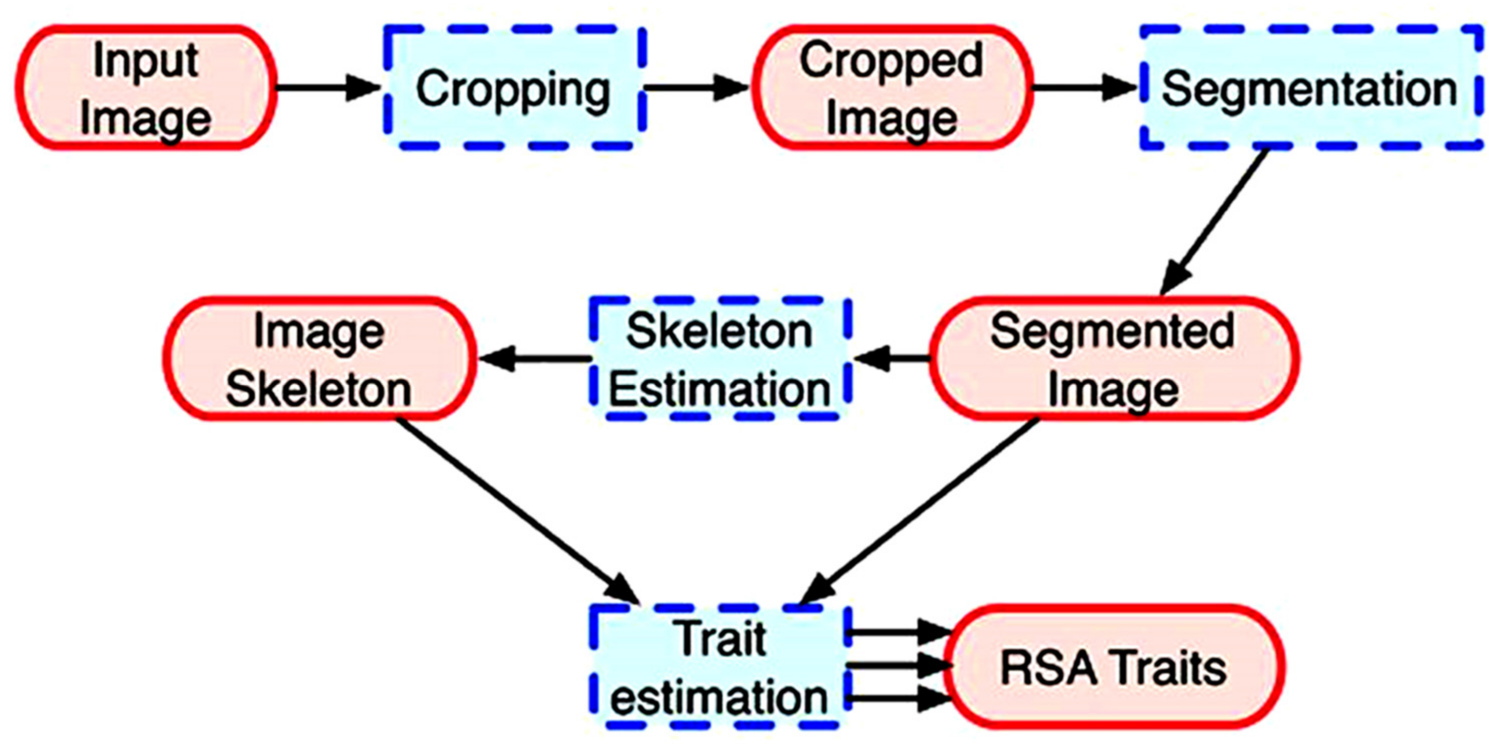
2.6. Image Acquisition, Analysis and Output

The camera was attached via a USB 2.0 port to a personal computer, and digital photographs were captured and saved. The root systems of individual seedlings were photographed after they were laid and distributed in a specimen tray with nutrient solution. After batch processing and analysis of the color RGB photos with the GiA Roots software (Figure 2). The software saved output as a comma separated value in csv extension file.

2.7. Recorded Data

Average root width (ARW): The average root-width estimation for the complete root system, calculated for all pixels along the medial axis.

Ellipse axis ratio (EAR): The ratio between the minor and major axes of an acceptable ellipse.

Major ellipse axis (MJEA): The length of the major axis of the ellipse that provides the best fit to the network.

The maximum number of roots (MANR): The 84th percentile value is determined by ordering the number of roots crossing a horizontal line from smallest to greatest, and the highest number is regarded as the maximum number.

The median number of roots (MENR): The result of a vertical line sweep (Figure S1), which evaluated the number of roots that crossed a horizontal line and then calculated the median of all values for the network’s extent.

Minor ellipse axis (MIEA): The length of the minor axis of the ellipse that provides the best fit to the network.

Network area (NWA): The number of network pixels in the image.

Network bushiness (NWB): The ratio of the maximum to the median number of roots.

Network convex area (NWCA): The area of the convex hull that encompasses the image.

Network depth (NWD): The vertical distance between the top-most network pixel and the bottom-most network pixel in pixels.

Network length (NWL): Number of pixels in the skeleton network, in whole or in part.

Network length distribution (NWLD): The proportion of network pixels that are located in the lower two-thirds of the network. The bottom two-thirds of the network is specified by the network depth.

Network perimeter (NWP): The sum of all pixels that are related to a backdrop pixel (using an 8-nearest neighbor neighborhood).

Network solidity (NWS): The entire network region is separated by the network’s convex area.

Network surface area (NWSA): The total of the local surface areas at each pixel in the network’s skeleton, approximated as a tubular shape with an image-derived radius.

Network volume (NWV): The total of the local volumes at each pixel in the network skeleton, approximated as a tubular shape with an image-derived radius.

Network width (NWW): The number of pixels in the horizontal direction from leftmost network pixel to the rightmost network.

Network width to depth ratio (NWWDR): The width of the network divided by the depth of the network.

The number of connected components (NCC): After picture preprocessing, an integer indicating the number of connected groups of network pixels in the image.

Specific root length (SRL): Total root length divided by the volume of the root system. Volume is estimated as the total of the cross-sectional areas of all pixels along the root system’s medial axis. The total root length is the number of pixels in the root system’s medial axis.

2.8. Statistical Analysis

A linear model in alpha-lattice design [26] with four replications was used for individual and combined analysis. R-statistics software Version 3.0.2 for Windows was used for statistical analysis [27]. Analysis of variance was utilized to estimate components of phenotypic variance for each variable using constrained maximum likelihood approaches. To estimate variance components, the lme4 package’s linear mixed effect “lmer” function was used.

2.8.1. Best Linear Unbiased Predictors (BLUPs)

In order to calculate BLUPs, the very same models that were utilized to compute variance components were applied for every line and each character. The lme4 package’s random effect “ranef” command was used to calculate BLUPs for all model terms. The agricolae R-package was used to assess the genotypic, phenotypic, and broad-sense heritabilities.

2.8.2. Multivariate Analysis

All pairs of entries had their Euclidean distance coefficients evaluated using the software Version 2.0.1 of the Statistical Tool for Agricultural Research (STAR) which is developed by the International Rice Research Institute. A Euclidean distance matrix built from data on seedlings was utilized as input for cluster analysis by the unweighted pair group method of arithmetic average (UPGMA) and for principal component analysis (PCA) to identify the primary features responsible for the majority of the gross variance seen between the examined inbred lines. To evaluate the relatedness of lines, a UPGMA dendrogram was created using Euclidean genetic distances.

2.8.3. Genotype by Trait (GT) Interactions Biplot

The comparative trait value for every trait was derived by dividing it by the related trait value obtained from the NP treatment. STAR software was used to create a GT biplot from a two-way matrix of eight traits and 220 genotypes using the relative trait. The first two principal components were plotted. Genotypes were plotted using the principal component scores, while characteristics were plotted using the principal component eigenvectors.

2.8.4. Multi-Trait Index Based on Factor Analysis and Genotype-Ideotypes Distance (MGIDI)

Olivoto and Nardino [28] proposed a multi-trait score based on component analysis and genotype-ideotypes distance (MGIDI) to identify novel donors capable of performing well under both optimal and low nitrogen environments. Additionally, the MGIDI index result was compared to the result of the Smith-Hazel (SH) index developed by Smith [29] and Hazel [30] and the ideotypes-design (FAI-BLUP) index suggested by Rocha et al. [31].

3. Results

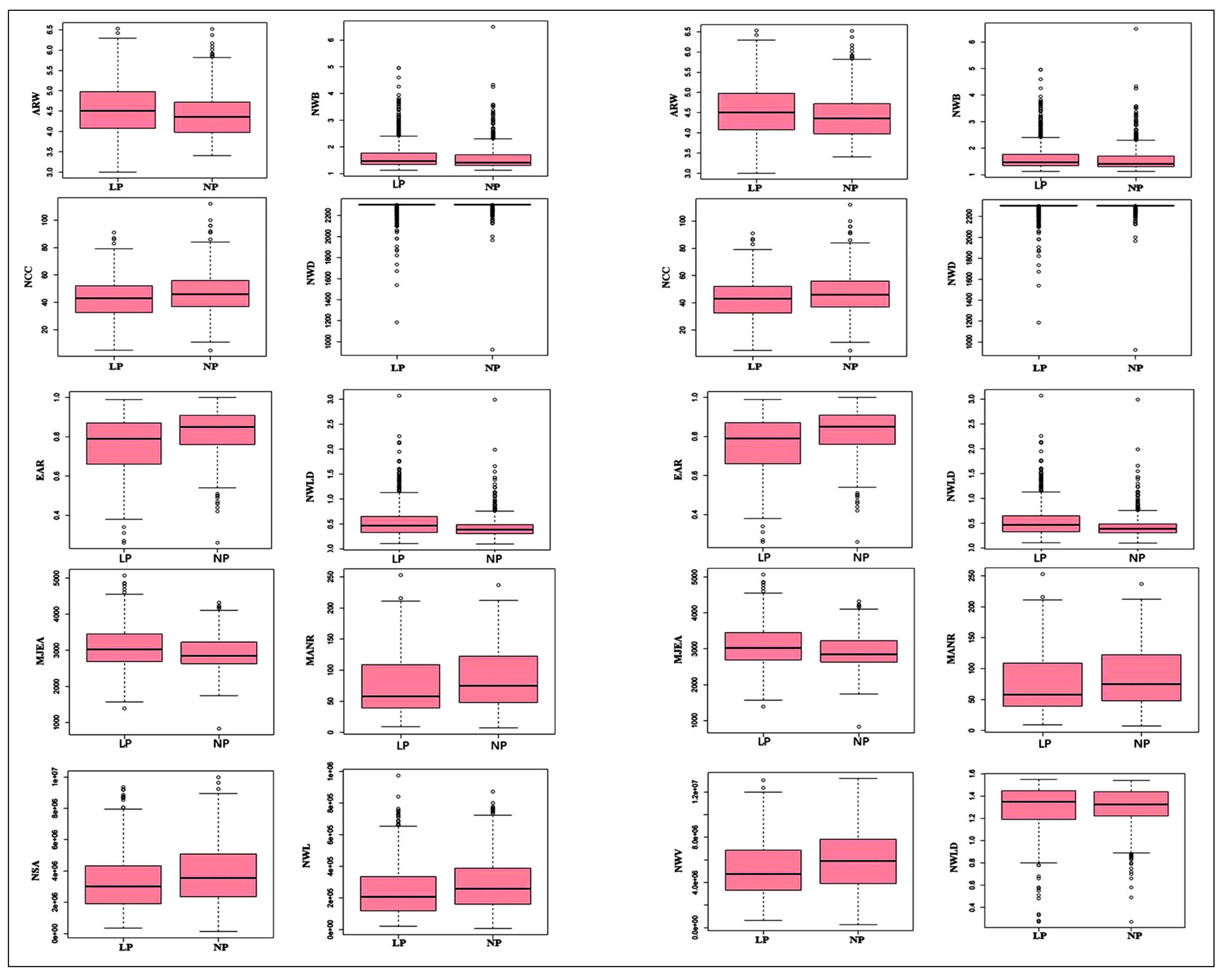
3.1. Descriptive Statistic and Analysis of Variance

For each root network trait (RNT), descriptive statistics including means with their standard errors are summarized in Table 1. For most traits, higher means were observed under LP. RAS development was found to be more prominent under LP, which is evident from the increase in NCR, EAR, MANR, NWW, MINR, MEA, NWA, NCA, NWS, NSA, NWV, and NWDR. For all traits measured by GiA Roots, a wide variety of phenotypic values was detected (

Table 3. Descriptive statistics for tested traits under LP and NP treatments.

Traits	Treat.	Mean	SE	Minimum	Maximum	Median	Mode	Kurtosis	Skewness
ARW	NP	4.52	0.02	3.00	6.53	4.44	6.01	−0.38	0.46
	LP	4.45	0.02	3.41	6.52	4.40	4.12	−0.05	0.62
NWB	NP	1.62	0.01	1.12	4.96	1.45	1.50	7.91	2.50
	LP	1.54	0.01	1.10	6.50	1.39	1.33	20.68	3.40
NCC	NP	43.89	0.42	3.00	91.00	44.00	43.00	−0.11	0.13
	LP	46.15	0.37	5.00	112.00	45.00	44.00	0.64	0.38
NWD	NP	2290.35	2.17	910.00	2303.00	2303.00	2303.00	158.25	−11.45
	LP	2297.84	1.25	926.00	2303.00	2303.00	2303.00	634.59	−22.55
EAR	NP	0.76	0.00	0.11	0.99	0.79	0.84	−0.24	−0.56
	LP	0.82	0.00	0.26	1.00	0.85	0.84	0.24	−0.87
NWLD	NP	0.53	0.01	0.11	3.07	0.46	0.24	8.27	2.20
	LP	0.44	0.01	0.06	2.99	0.41	0.61	26.59	3.20
MJEA	NP	3105.60	15.08	823.57	5072.72	3001.58	2632.98	0.05	0.47
	LP	2972.72	11.85	830.81	4465.25	2856.90	2679.85	0.33	0.66
MANR	NP	77.86	1.25	5.00	253.00	62.00	56.00	−0.51	0.64
	LP	83.14	1.24	7.00	237.00	69.00	44.00	−0.55	0.70
NWW	NP	2956.82	13.59	179.00	3455.00	3116.00	3455.00	3.19	−1.54
	LP	2979.72	11.07	249.00	3455.00	3046.00	3455.00	2.48	−1.22
MENR	NP	52.43	0.97	2.00	223.00	42.00	21.00	0.52	1.02
	LP	57.32	0.97	4.00	177.00	45.00	37.00	0.48	1.08
MIEA	NP	2310.48	7.83	239.24	2972.45	2353.58	2201.84	8.46	−1.97
	LP	2386.18	6.64	213.02	3162.82	2398.86	2255.16	7.44	−1.09
NWA	NP	85,2169.61	12,698.0	28,448.00	2,306,467.00	766,588.00	425,187.00	−0.21	0.67
	LP	927,120.77	12,626.3	33,913.00	2,380,819.00	828,074.00	1,399,665.00	−0.15	0.72
NWCA	NP	6,256,640.0	33,659.7	331,902.00	7,899,088.00	6,517,483.75	4,864,456.50	2.12	−1.20
	LP	6,326,244.7	26,555.5	148,855.50	7,907,468.00	6,493,552.25	4,333,747.00	2.02	−0.99
NWP	NP	419,776.22	7310.85	10,665.00	1,449,259.00	346,500.50	149,445.00	0.20	0.88
	LP	455,401.13	7309.86	11,192.00	1,372,171.00	375,264.00	709,723.00	0.21	0.95
NWS	NP	0.14	0.00	0.02	0.47	0.12	0.09	0.84	1.11
	LP	0.15	0.00	0.03	0.46	0.13	0.32	0.23	1.00
SRL	NP	0.05	0.00	0.02	0.10	0.04	0.03	0.43	0.70
	LP	0.05	0.00	0.02	0.08	0.05	0.05	−0.61	0.27
NWSA	NP	3,523,843.5	53,442.4	109,925.66	9,490,765.02	3,153,257.77	1,669,954.28	−0.20	0.69
	LP	3,832,697.7	53,021.9	127,452.83	10,048,319.6	3,407,774.88	5,810,109.73	−0.12	0.73
NWL	NP	265,436.89	4685.19	6132.00	975,158.00	219,807.50	88,374.00	0.23	0.89
	LP	287,929.75	4665.79	6225.00	879,854.00	238,309.00	449,101.00	0.24	0.96
NWV	NP	5,462,435.1	71,955.11	204,831.84	13,046,946.3	5,082,050.76	3,397,327.72	−0.53	0.43
	LP	5,916,641.1	70,714.1	256,796.93	13,200,212.0	5,630,054.48	8,591,461.09	−0.62	0.39
NWWDR	NP	1.29	0.01	0.12	1.57	1.35	1.50	2.52	−1.41
	LP	1.30	0.00	0.27	1.68	1.32	1.50	1.79	−1.13

ARW = Average root width, NWB = Network bushiness, NCC = Number of connected components, NWD = Network depth, EAR = Ellipse axis ratio, NWLD = Network length distribution, MJEA = Major ellipse axis, MANR = Maximum number of roots, NWW = Network width, MENR = Median number of roots, MIEA = Minor ellipse axis, NWA = Network area, NWCA = Network convex area, NWP = Network perimeter, NWS = Network solidity, SRL = Specific root length, NWSA = Network surface area, NWL = Network length, NWV = Network volume, NWWDR = Network width to depth ratio.

).

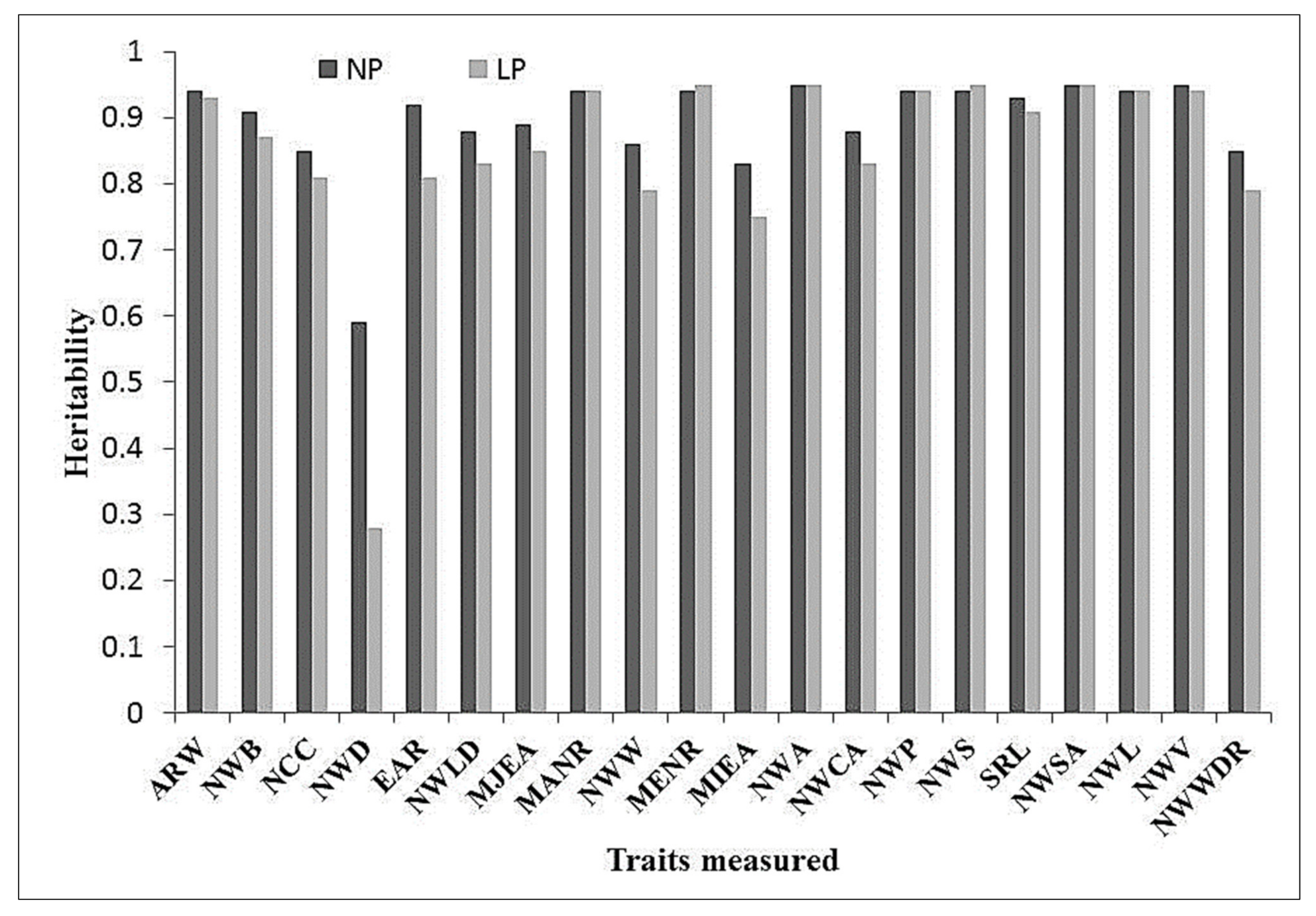
3.2. Analysis of Variance and Broad-Sense Heritability Estimated

Mixed model analysis revealed significant differences (p ≤ 0.01) in all evaluated RNS features between inbred lines in the LP and NP treatments (

Table 4. Analysis of variance of the different RNS tested traits.

Traits	Treatment	Mean Square			F-Value (Gen)	Significance Level
		Replication	Genotype	Error
ARW	NP	0.04	1.45	0.09	15.69	***
	LP	0.02	0.93	0.07	14.2	***
NWB	NP	0.04	0.78	0.07	10.83	***
	LP	0.07	0.61	0.08	7.78	***
NCC	NP	13.07	648.64	95.46	6.80	***
	LP	83.32	482.43	93.30	5.17	***
NWD	NP	161.82	11,386.40	4695.10	2.43	***
	LP	838.02	2807.12	2030.71	1.38	*
EAR	NP	0.01	0.06	0.01	12.7	*
	LP	0.01	0.03	0.01	5.30	***
NWLD	NP	0.03	0.27	0.03	8.11	***
	LP	0.01	0.11	0.02	6.03	***
MJEA	NP	76,230.1	916,523	103,873	8.82	***
	LP	99,507.1	486,751	71,573.5	6.80	***
MANR	NP	12.857	7172.570	442.848	16.2	***
	LP	229.32	7031.23	456.18	15.41	***
NWW	NP	64,219.4	696,475	100,280	6.95	***
	LP	57,281.70	407,323.00	85,124.00	4.79	***
MENR	NP	12.86	7172.57	442.85	16.2	***
	LP	229.32	7031.23	456.18	15.41	***
MIEA	NP	76,230.1	916,523	103,873	8.82	***
	LP	99,507.10	486,751.00	71,573.50	6.80	***
NWA	NP	851,326,000.00	756,240,000,000.00	38,367,000,000.00	19.71	***
	LP	27,187,900,000.00	761,409,000,000.00	40,363,800,000.00	18.86	***
NWCA	NP	663,782,000,000.00	4,530,370,000,000.00	528,786,000,000.00	8.57	***
	LP	217,830,000,000.00	2,475,580,000,000.00	428,953,000,000.00	5.77	***
NWP	NP	120,272,000.00	246,041,000,000.00	14,265,200,000.00	17.25	***
	LP	9,820,570,000.00	252,527,000,000.00	14,005,400,000.00	18.03	***
NWS	NP	0.001	0.025	0.001	16.83	***
	LP	0.001	0.026	0.001	19.64	***
SRL	NP	0.00003	0.00055	0.00004	14.78	***
	LP	0.00001	0.00036	0.00003	13.06	***
NWSA	NP	12,716,500,000.00	13,361,400,000,000.00	690,971,000,000.00	19.34	***
	LP	523,286,000,000.00	13,377,900,000,000.00	721,558,000,000.00	18.54	***
NWL	NP	65,982,000.00	100,591,000,000.00	6,010,840,000.00	16.73	***
	LP	4,479,120,000.00	102,500,000,000.00	5,795,460,000.00	17.69	***
NWV	NP	120,369,000,000.00	24,219,600,000,000.00	1,252,990,000,000.00	19.33	***
	LP	902,056,000,000.00	23,414,500,000,000.00	1,350,090,000,000.00	17.34	***
NWWDR	NP	0.01	0.12	0.02	6.72	***
	LP	0.01	0.08	0.02	4.71	***

ARW = Average root width, NWB = Network bushiness, NCC = Number of connected components, NWD = Network depth, EAR = Ellipse axis ratio, NWLD = Network length distribution, MJEA = Major ellipse axis, MANR = Maximum number of roots, NWW = Network width, MENR = Median number of roots, MIEA = Minor ellipse axis, NWA = Network area, NWCA = Network convex area, NWP = Network perimeter, NWS = Network solidity, SRL = Specific root length, NWSA = Network surface area, NWL = Network length, NWV = Network volume, NWWDR = Network width to depth ratio. Significant differences (* p < 0.05, *** p ≤ 0.01).

).

An extensive range of phenotypic values was detected for all traits. The traits tested in this experiment were influenced by LP stress treatment, and the effect of LP and NP treatments on maize germplasm for measured traits are shown by box plots (Figure 3). The box plot’s edges depict the upper and lower quintiles, as well as the median, which is depicted in the box’s center. Elements that do not fit inside the rank of whisker are indicated by a circle.

Estimated heritabilities (h²) ranged from 59% to 95% under NP and 23% to 95% under LP. This difference reflects the relative amount of genetic variation among germplasm and was not consistent among the different types of RAS trait measurements (Figure 4). In general, h² estimates for ARW, MJNR, MINR, NWA, NWP, NWS, NSA, NWL, and NWV were typically greater than those associated with the other qualities investigated.

3.3. Variance Components

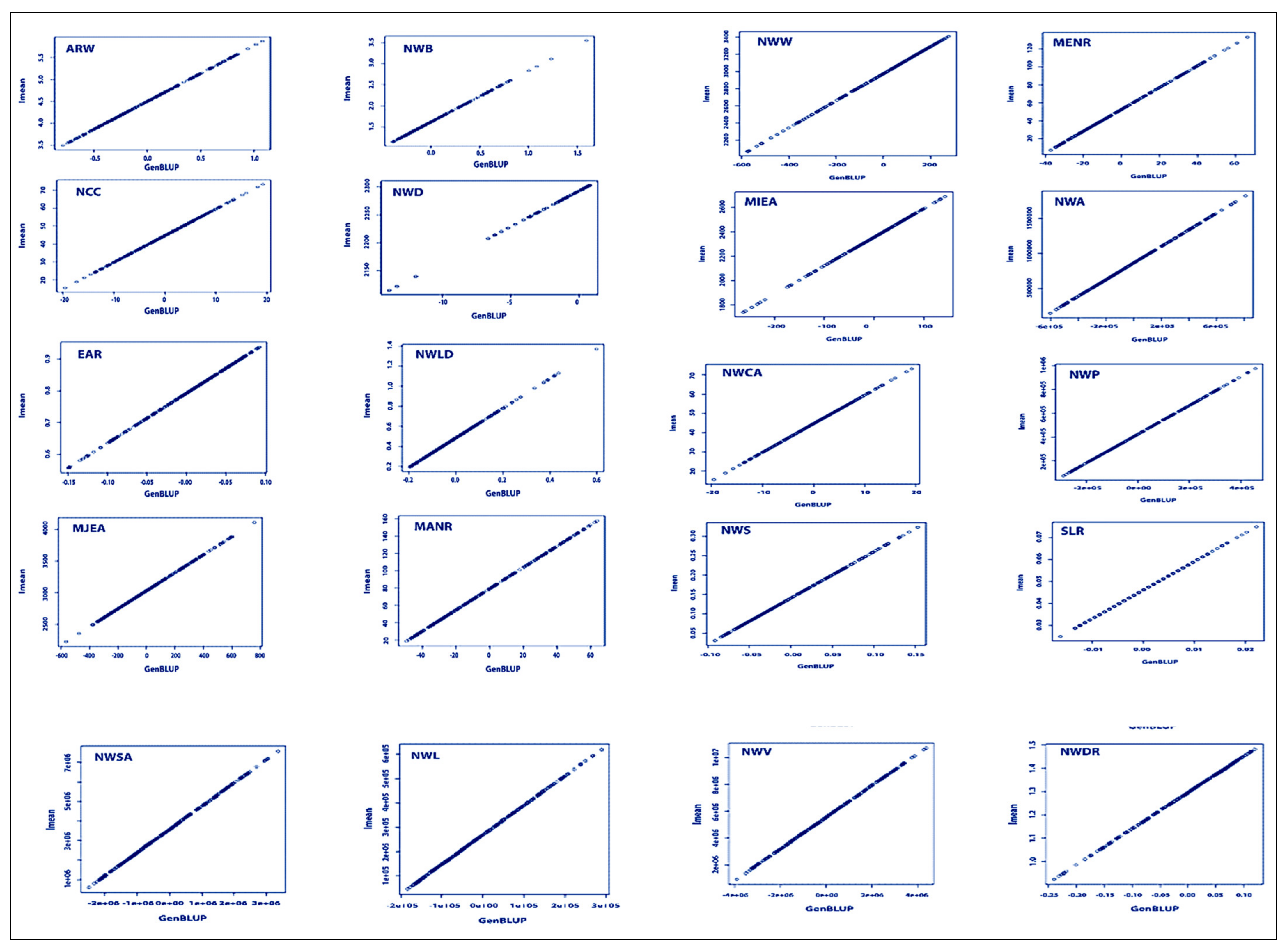
For each maintained trait, the variance components due to genotype, treatment (environment), and genotype-by-treatment interaction were evaluated (

Table 5. Estimates of variance components (proportion of the total).

Traits	Genotype	Genotype × Treatment	Treatment	Residual
ARW	0.53	0.24	0.03	0.21
NWB	0.53	0.14	0.01	0.33
NCC	0.32	0.21	0.05	0.41
NWD	0.01	0.14	0.01	0.84
EAR	0.30	0.26	0.11	0.33
NWLD	0.34	0.24	0.08	0.34
MJEA	0.37	0.22	0.04	0.37
MANR	0.55	0.20	0.03	0.22
NWW	0.29	0.20	0.00	0.50
MENR	0.56	0.19	0.03	0.21
MIEA	0.16	0.31	0.05	0.48
NWA	0.60	0.18	0.04	0.18
NWCA	0.39	0.18	0.01	0.42
NWP	0.57	0.19	0.04	0.20
NWS	0.58	0.18	0.03	0.21
SRL	0.50	0.24	0.01	0.26
NWSA	0.59	0.18	0.04	0.19
NWL	0.56	0.19	0.04	0.21
NWV	0.60	0.17	0.04	0.19
NWWDR	0.29	0.19	0.00	0.51

ARW = Average root width, NWB = Network bushiness, NCC = Number of connected components, NWD = Network depth, EAR = Ellipse axis ratio, NWLD = Network length distribution, MJEA = Major ellipse axis, MANR = Maximum number of roots, NWW = Network width, MENR = Median number of roots, MIEA = Minor ellipse axis, NWA = Network area, NWCA = Network convex area, NWP = Network perimeter, NWS = Network solidity, SRL = Specific root length, NWSA = Network surface area, NWL = Network length, NWV = Network volume, NWWDR = Network width to depth ratio.

). The proportions of genetic variance ranged from 0.01–0.60 for different maize RNS traits. The highest levels of genetic variance were found in NWA and NWV, and the lowest proportion of genetic variance was in NWD. Overall, ARW, NWB, MANR, MINR, NWP, NWS, SLR, NSA, and NWV were discovered to have a significantly high proportion of variance due to genetic effects, but a low proportion due to treatment effects.

3.4. BLUP Analysis

All attributes had their BLUPs assessed on a per-genotype basis. As expected, there was a substantial positive association between BLUPs and means, with the BLUPs gradually shrinking toward the population average (Figure 5).

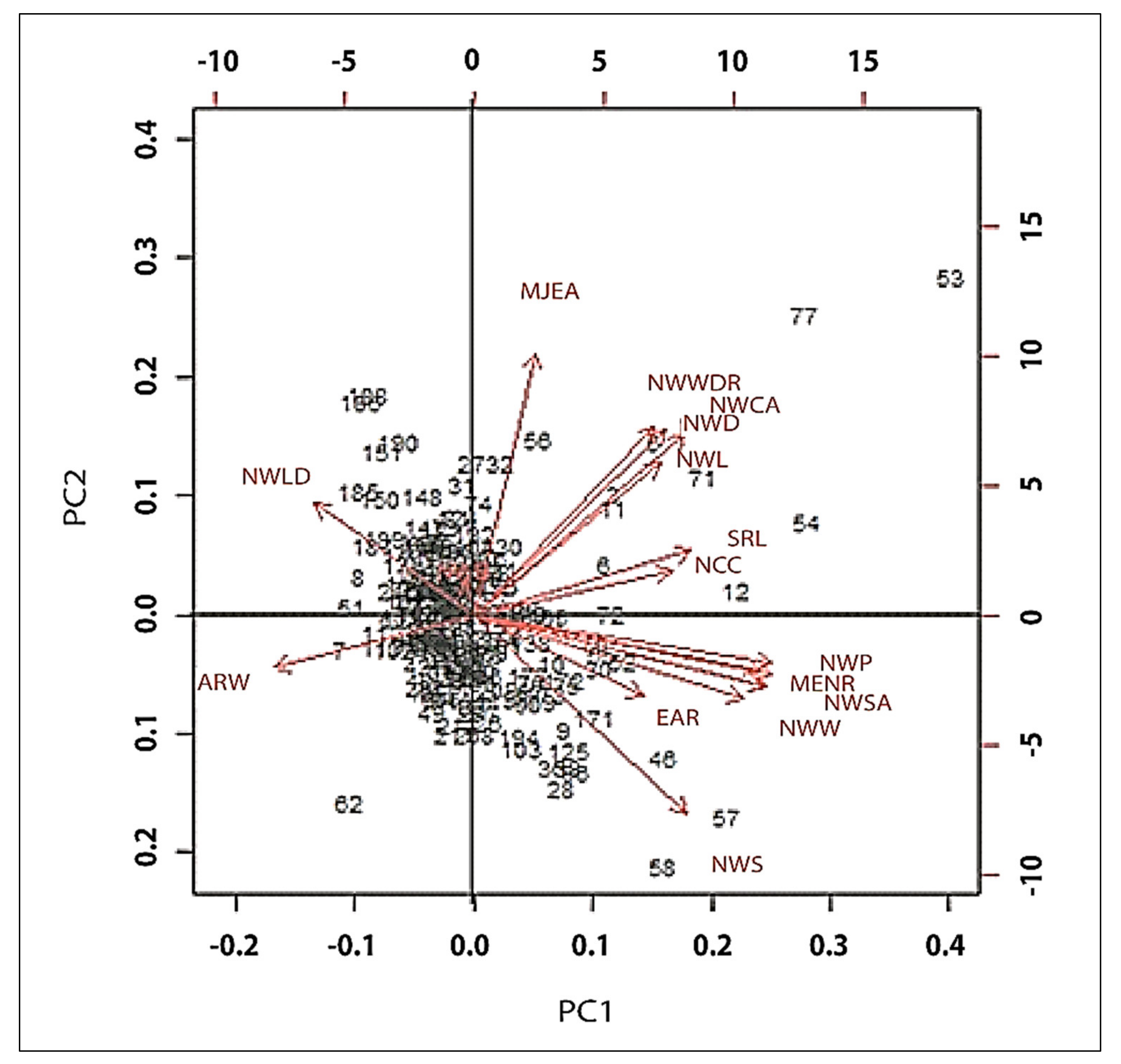
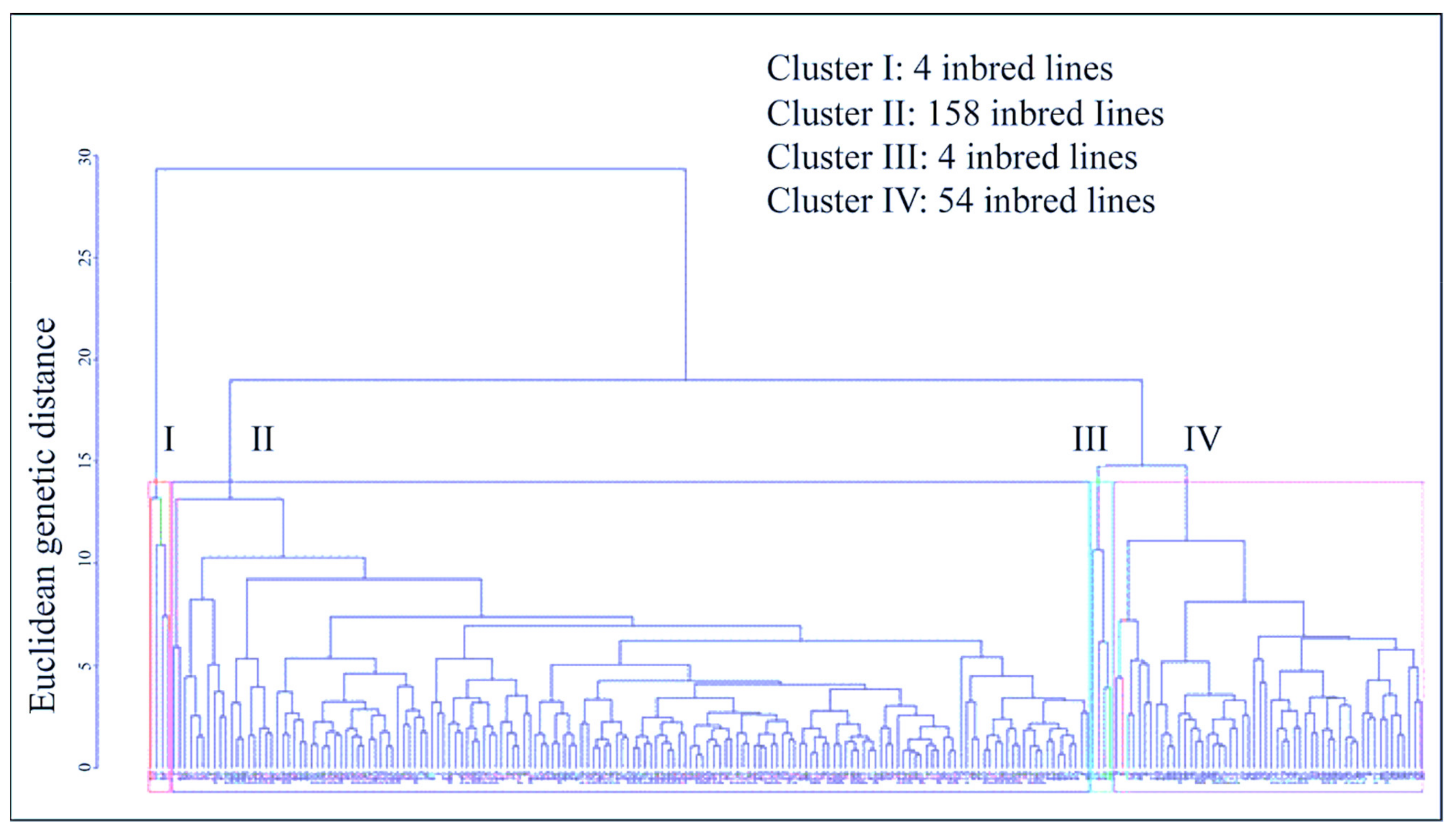
3.5. Multivariate Analysis

The first three PCs described around 79.27% of the overall dissimilarity among lines for the twenty RNS traits (

Table 6. The first four PCs of traits eigen vectors of the maize inbreds.

Parameter	PC1	PC2	PC3	PC4
ARW	−0.1955	−0.0387	0.2908	−0.3165
NWB	0.0163	0.0311	−0.2666	0.6438
NCC	0.2166	0.0606	0.2587	−0.0784
NWD	0.2171	0.2043	0.1941	0.1486
EAR	0.1465	−0.1705	0.4498	0.3054
NWLD	−0.1413	0.2499	−0.0488	−0.1898
MJEA	0.1008	0.4366	−0.2509	−0.2223
MANR	0.2823	−0.098	−0.1934	−0.0069
NWW	0.2087	0.2918	0.2853	0.1004
MENR	0.2823	−0.098	−0.1934	−0.0069
MIEA	0.1008	0.4366	−0.2509	−0.2223
NWA	0.2952	−0.1247	−0.0122	−0.1458
NWCA	0.2387	0.2501	0.2458	0.0917
NWP	0.2999	−0.0692	−0.0912	−0.0696
NWS	0.1752	−0.3885	−0.0632	−0.16
SRL	0.2249	0.046	−0.3095	0.2565
NWSA	0.2957	−0.1204	−0.016	−0.1436
NWL	0.2999	−0.0651	−0.0875	−0.074
NWV	0.2685	−0.1737	0.0867	−0.2503
NWWDR	0.1947	0.3003	0.2624	0.0654
Cumulative% of total variance	52.18	69.24	79.84	85.71

ARW = Average root width, NWB = Network bushiness, NCC = Number of connected components, NWD = Network depth, EAR = Ellipse axis ratio, NWLD = Network length distribution, MJEA = Major ellipse axis, MANR = Maximum number of roots, NWW = Network width, MENR= Median number of roots, MIEA = Minor ellipse axis, NWA = Network area, NWCA = Network convex area, NWP = Network perimeter, NWS = Network solidity, SRL = Specific root length, NWSA = Network surface area, NWL = Network length, NWV = Network volume, NWWDR = Network width to depth ratio.

). The comparative magnitude of eigenvectors for the first principal component was 50.51%, clarified mostly by NCC, NWD, MJEA, NWW, MIEA, NWCA, SRL, and NWWDR. From the second and third principal components, which donated 18.83% and 9.93% of the entire variation, respectively, the most predominant traits were NWLD, NWD, NWCA, NWW, and NWWDR.

Based on RNS characteristics, Euclidian distance coefficients were determined for all inbred lines of maize (Figure 6).

Cluster analysis identified two distinct clusters among the 220 inbred lines. The first cluster had 216 lines with relatively minor RNS characteristics, whereas the second cluster comprised four inbred lines (CML 331/MBR, CML 311, 3130 and CML96) which had extreme relative values like NCC, NWD, EAR, MJEA, MANR, NWW, MENR, MIEA, NWA, NWCA, SRL, NWL, and NWWDR. The first cluster was distributed into three subgroups. The first subgroup contained 158 lines which displayed the lowest NWB, NCC, NWD, EAR, MJEA, MANR, NWW, MENR, MIEA, NWA, NWCA, NWP, NWS, SRL, NWSA, NWL, NWV, and NWWDR, whereas the second subgroup contained 54 lines with moderate values of NWB, NCC, NWD, EAR, MJEA, MANR, NWW, MENR, MIEA, NWA, NWCA, NWP, NWS, SRL, NWSA, NWL, NWV, and NWWDR. The second subgroup contained only four lines (E28, CML 300, CML319 and CML 322) with high MANR, MENR, NWA, NWP, NWS, NWSA, and NWV. The genetic distance mean was 5.34, ranging from 0.61 to 29.33. The maximum genetic distance (29.33) was acquired between inbreds 53 and 62.

3.6. Genotype by Trait Interactions

A G × T biplot was created using relative traits from a two-way matrix of 20 RNS traits by 220 genotypes (Figure 7).

The graphic reduced the information from this matrix into two main components, the first two of which accounted for 69.24% of the overall variation. The graph depicts the link between qualities. The correlation coefficient between qualities is proportional to the cosine of the angle between vectors relating those traits to the source. Qualities on differing sides of the source are thus negatively interrelated, traits close to each other are favorably associated, and traits at 90° to each other to the source are not connected. The GT biplot reveals superior genotypes with favorable trait combinations. The findings indicate that NWD, NWCA, NCC, SRL, MJEA, NWW, and NWCA may be useful in identifying superior genotypes in elite germplasm.

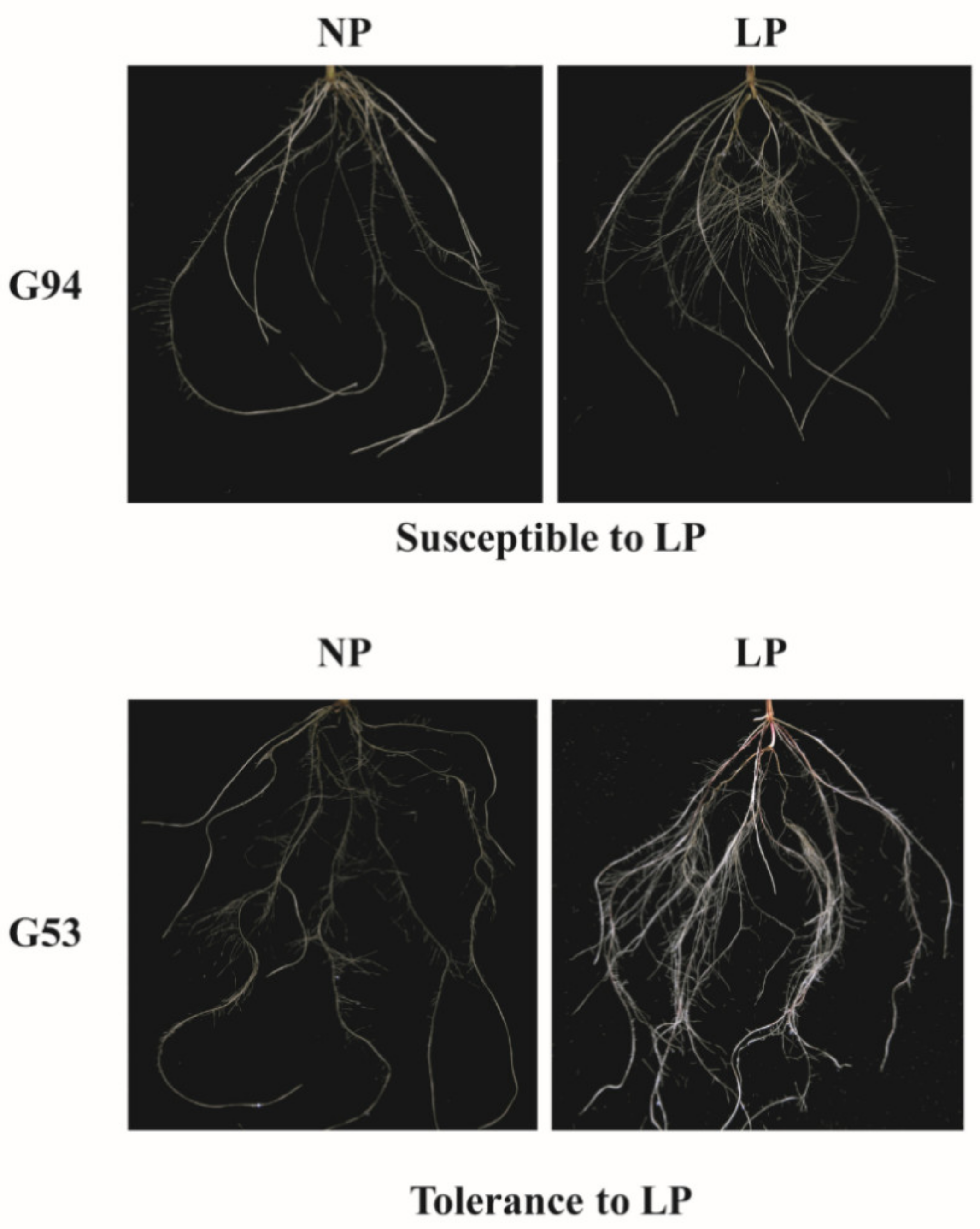
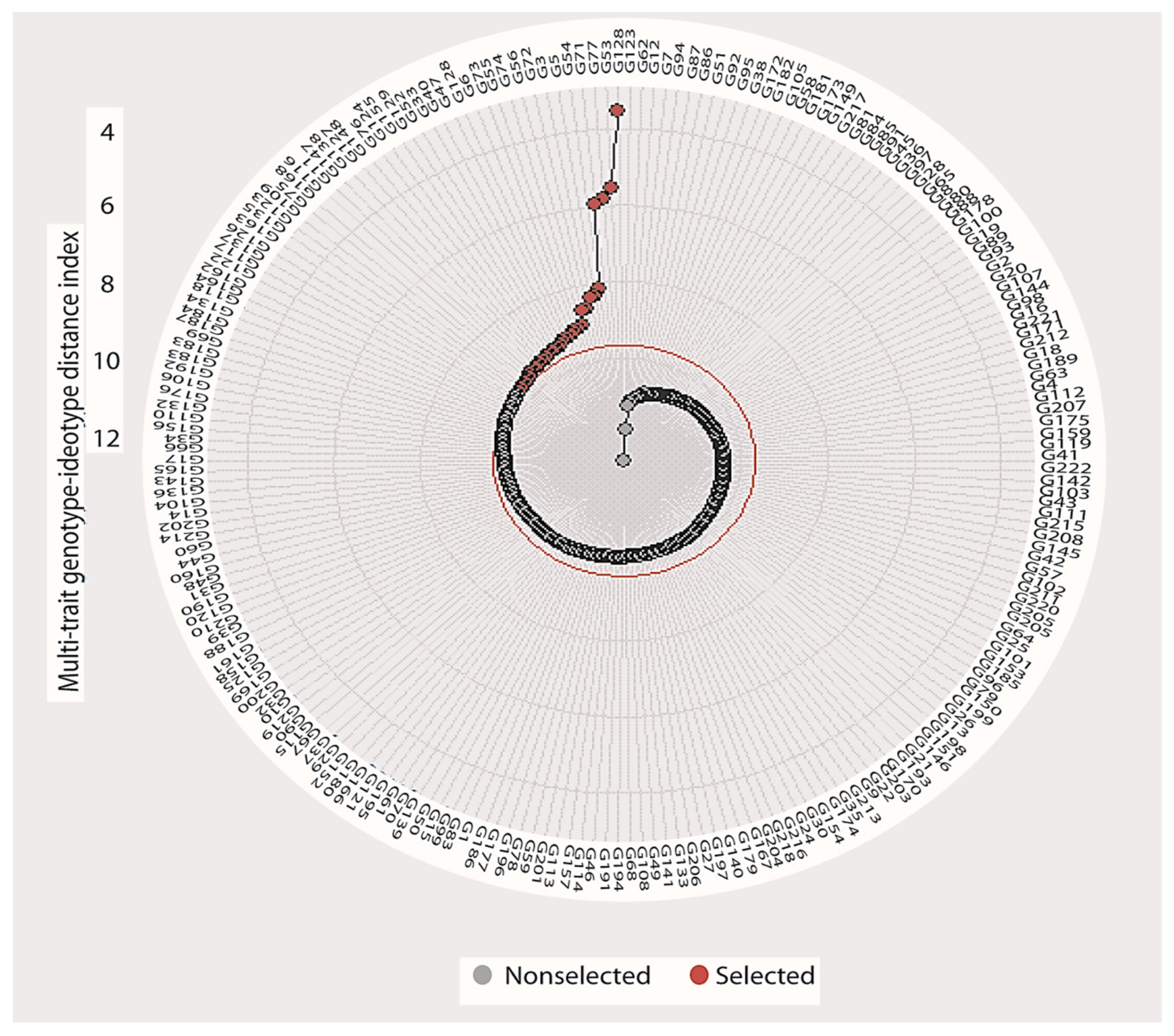
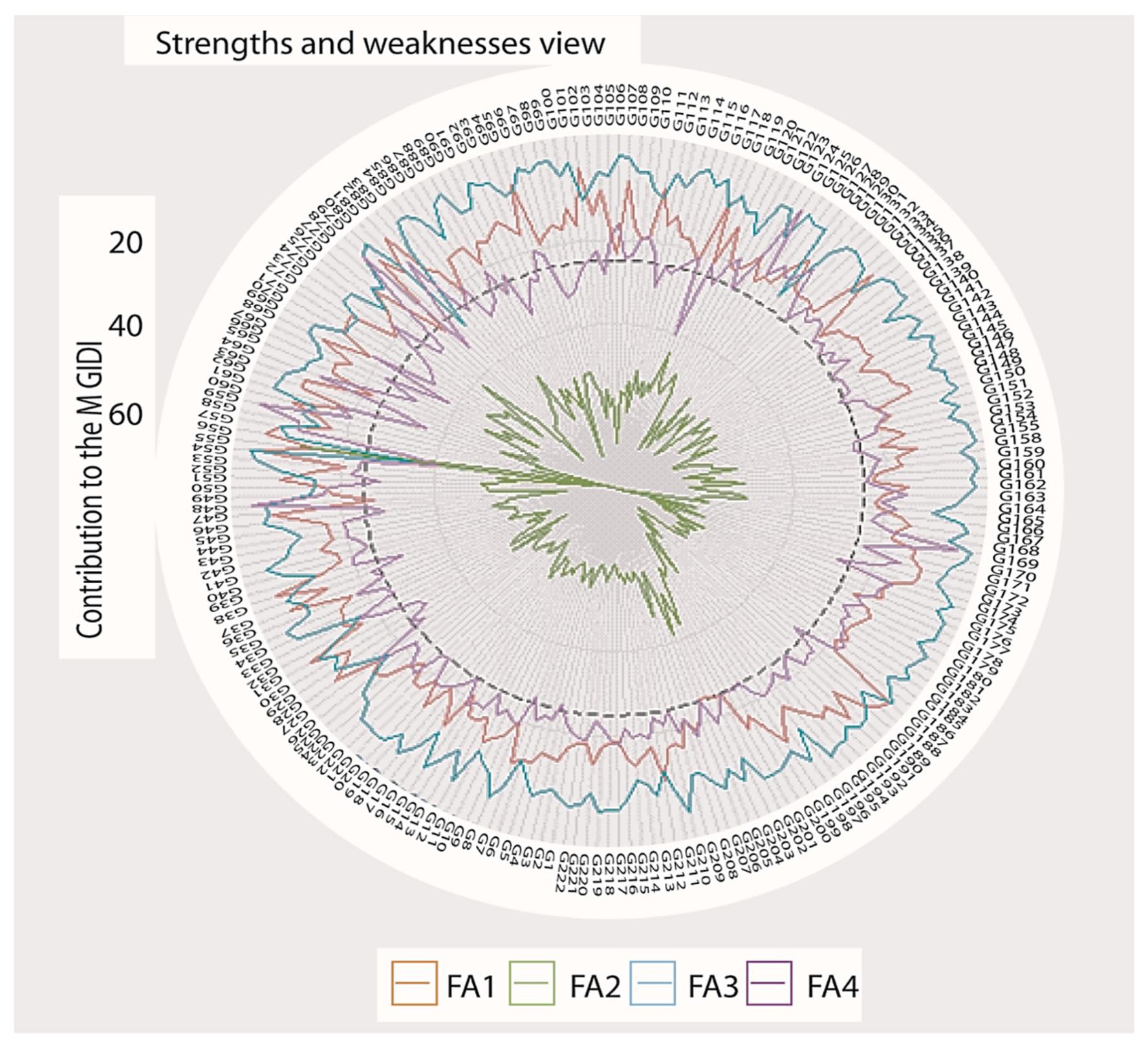
3.7. Multi-Trait Index Based on Factor Analysis and Genotype-Ideotype Distance (MGIDI)

The MGIDI index was intended to select the genotypes with respect to considering all measured traits. Based on the analysis, a highly significant genotypic consequence was noted for all measuring traits (Table 1). Under NP, estimated heritabilities (h²) ranged from 59 to 95%, while under LP, they ranged from 23 to 95%. This difference reflects the relative amount of genetic variation among germplasm and was not consistent across RAS trait measurements (Figure 4). ARW, MJNR, MINR, NWA, NWP, NWS, NSA, NWL, and NWV h2 estimates were consistently greater than those for the other qualities investigated. However, the genotypes selected using the MGIDI index were G53, G77, G71, G54, G5, G3, G72, G56, G74, G55 and G73 (Figure 8). The strengths and weaknesses of each genotype were depicted in Figure 9.

4. Discussion

Significant quantitative variations in a variety of seedling features were detected when seedlings were evaluated under LP and NP circumstances in a high-lux plant development environment, showing a significant degree of morphological variation in the maize germplasm panel investigated. Maize accessions with extended MSL, MRL, and RSR discovered in this experiment are promising candidates for LP tolerance breeding. Similarly, multiple investigations have revealed significant variation in maize inbreds, with tolerant inbreds having longer roots, more root volume and leaf area, and more root hairs than sensitive inbreds under P shortage conditions [5,32,33,34,35,36]. During the seedling stage, LP tolerant genotypes displayed a low shoot dry-weight, a robust root system, and a high root to shoot ratio [37,38,39,40,41,42]. This is because a robust root system enables plants to develop more rapidly and fully prior to LP stress, hence speeding P-scavenging and sustaining growth at the seedling stage in LP surroundings. Additionally, a robust RAS with an extensive and well-distributed root system is critical for the uptake of both mobile and immobile nutrients, such NO₃ [43] and P. This is because the root system will graze in a larger area of soil, increasing nutrient intake.

Hydroponic evaluation of maize germplasm enables the identification of maize lines with improved root properties [44]. While this method can be used to analyze seedlings as young as 14 days, the measures acquired can be utilized to predict lines with superior root development at later stages of development. Environmental impacts on plants in the field were also a disadvantage in identifying superior phenotypes, making the hydroponic assessment under controlled settings more trustworthy. Another benefit of the hydroponic approach is that it allows for the screening of a high number of lines using a tiny growing chamber. However, numerous downsides of hydroponic systems should be mentioned, including abnormal root conditions and the inability to bring plants to maturity [45]. Furthermore, according to Tuberosa et al. [46], when it comes to identifying quantitative trait loci (QTL) for characteristics like root traits, the magnitude and nature of the “QTL environment” interactions are more important than the absolute values of root attributes evaluated in hydroponics. As a result, if common QTL for root qualities developed in hydroponics and the field could be found, those QTL could have an impact on grain yield. Many plants, including rice, maize, and soybean, have been studied genetically for LP tolerance utilizing biparental populations [47,48,49]. Various characteristics have been utilized in maize to investigate the genetic basis of LP tolerance. RIL populations were used to conduct QTL analyses for root hair length, seminal root length and number, and lateral root length and number under LP and NP conditions [50,51,52].

For the most part, the estimated genetic components of variance were low to moderate. The modest genetic variations could be due to the fact that the germplasm panel included cultivars and breeding lines that had undergone extensive selection. The low genetic variance could also indicate a complex genetic inheritance pattern and/or a high environmental influence on characteristic manifestation. Complex root features, such as lateral root, seminal root, and root hair are genetically controlled by multi-gene or QTL and/or loci with epistatic effects, according to previous QTL studies conducted in the context of biparental mapping [49,53,54].

Enhancing selection techniques for quantitative trait improvement requires accurate estimates of the heritability and variance components of selection gain. The large genetic variations and moderate-to-high heritability estimates discovered in this work for many seedling trait qualities imply promising prospects for increasing adult plant height and root length by the phenotypic selection, and consequently LP tolerance [55,56,57].

Correlation analysis of seedling traits under both LP and NP conditions revealed that genotypic correlation coefficients were frequently greater than corresponding phenotypic correlation coefficients, indicating that the suppressive effect of the treatment altered phenotypic expression by lowering phenotypic correlation coefficient values. In a few cases, the phenotypic correlation coefficients were equal to or greater than the genotypic correlation coefficients, implying that both treatment and genotypic correlations act in the same direction and ultimately maximize phenotypic expression.

PCA demonstrated that seedling traits, such as MSL, MRL, RDW, and RSR account for the majority of phenotypic variations, implying that these traits account for most of the diversity observed between the maize accessions tested. Concentrating on MSL, RL, and root fresh weight appeared to be sufficient to account for variation between maize accessions at the seedling phase, and to identify a large number of lines for LP tolerance in future research. Due to the ease with which MSL can be measured in comparison to other traits, it might be used as an indirect attribute to describe TDM. In various screening trials, the relative-trait method is the most reliable method for classifying LP tolerance [18,58,59].

Generally, the methods for evaluating root traits are incapable of being actualized up for high-throughput applications. The GiA Roots (General Image Analysis of Roots) is a software application that automates and facilitates the analysis of root networks on a large scale. It was created to assist scientists and breeders in assessing the structure of plant root-system architecture regardless of their prior mathematics or computer science training [60]. It can estimate quantitative features from photos of plant root networks with high accuracy. A high-throughput phenotyping technology enables rapid evaluation of a large number of plants and accurate measurement of attributes. By increasing the accuracy of phenotyping and analyzing a larger number of plants, we can reduce the standard error, giving us greater confidence in the mean value of the measured characteristic. Significant quantitative variation was reported for a variety of root-network system features examined under LP and NP circumstances in a high-lux plant growing room, demonstrating that root properties are very variable among inbred lines of maize. The inbred lines of maize employed in this investigation did not group according to their genetic backgrounds and origins, demonstrating a significant degree of diversity between and within distinct genetic backgrounds. Maize accessions with a long and enlarged root system revealed in this work are promising for LP tolerance breeding and for finding the genetic areas regulating these features. Breeders with experience frequently strive to blend multiple desired features into a new genotype to achieve high performance. When many attributes are measured, it is usually difficult to distinguish a genotype from an ideotype. Numerous multivariate methods, like principal component analysis, factor analysis, cluster analysis, and multiple samples, are commonly employed in this context to classify observed traits or to choose test genotypes [61]. In this study, a two-way heat map clustering pattern and PCA were used to connect test genotypes and measured attributes (Figure 6 and Figure 7), but we were not able to select the specific genotypes. Olivoto and Nardino [28] recently introduced MGIDI (multi-trait genotype-ideotypes distance index), a new technique for genotype isolation based on multiple trait information, to make the selection of genotypes with multiple features easier. The MGIDI index identified eggplant genotypes G53, G77, G71, G54, G5, G3, G72, G56, G74, G55, and G73 as promising. The use of the MGIDI index in plant crop research is expected to increase rapidly. Similarly, this index was employed in order to identify the best strawberry genotype [62].

5. Conclusions

In genetics and developmental biology, maize is a well-established model species. P is an indispensable constituent for the growth of plants. Because soil P availability is generally poor, a lot of phosphorus fertilizer is used to boost crop yields. P shortage in maize crops is common and reduces yields. For sustainable agriculture and global food security, breeding P efficiency in maize is critical. The inbred lines were grown up to 15 days in the high-lux plant growth room on hydroponic with LP and NP treatments after germination. The analysis of variance revealed a wide range of variability present among the inbred lines with intermediate to high heritabilities ranging from 0.59 to 0.95 for all RNS traits, specifying stability through the experiments. The proportions of genetic variance ranged from 0.01–0.60 in different maize RNS traits. Strong positive linear relationships between BLUPs were detected for all RNS traits. The Euclidean genetic distances ranged from 0.61 to 29.33, showing a high degree of variation among the inbred lines studied. The first three principal components described approximately 79% of the overall genetic variation, with high loadings from network length (NWL), network surface area (NWSA), network perimeter (NWP), network area (NWA), the maximum number of roots (MANR), median number of roots (MENR), network volume (NWV), network convex area (NWCA), specific root length (SRL), network depth (NWD), number of connected components (NCC), and network width (NWW). The genotype by trait interaction biplot revealed superior genotypes with more desirable trait interactions. Some outstanding genotypes (G53, G77, G71, G54, G5, G3, G72, G56, G74, G55, and G73), with higher values of most RNS traits, were identified using MGIDI analysis. These lines may be useful for breeding LP-tolerant maize.

References

1. Bailey-Serres, J.; Parker, J.E.; Ainsworth, E.A.; Oldroyd, G.E.D.; Schroeder, J.I. Genetic strategies for improving crop yields. Nat. Cell Biol. 2019, 575, 109–118. [Google Scholar] [CrossRef] [PubMed] [Green Version]
2. Raza, A.; Razzaq, A.; Mehmood, S.S.; Zou, X.; Zhang, X.; Lv, Y.; Xu, J. Impact of Climate Change on Crops Adaptation and Strategies to Tackle Its Outcome: A Review. Plants 2019, 8, 34. [Google Scholar] [CrossRef] [PubMed] [Green Version]
3. Yee, M.O.; Kim, P.; Li, Y.; Singh, A.K.; Northen, T.R.; Chakraborty, R. Specialized Plant Growth Chamber Designs to Study Complex Rhizosphere Interactions. Front. Microbiol. 2021, 12, 625752. [Google Scholar] [CrossRef] [PubMed]
4. FAO. The Future of Food and Agriculture—Trends and Challenges; Annual Report; FAO: Rome, Italy, 2017; p. 296. [Google Scholar]
5. Jia, X.; Liu, P.; Lynch, J.P. Greater lateral root branching density in maize improves phosphorus acquisition from low phosphorus soil. J. Exp. Bot. 2018, 69, 4961–4970. [Google Scholar] [CrossRef] [PubMed] [Green Version]
6. Zhang, L.; Yan, C.; Guo, Q.; Zhang, J.; Ruiz-Menjivar, J. The impact of agricultural chemical inputs on environment: Global evidence from informetrics analysis and visualization. Int. J. Low-Carbon Technol. 2018, 13, 338–352. [Google Scholar] [CrossRef] [Green Version]
7. Cordell, D.; White, S. Tracking phosphorus security: Indicators of phosphorus vulnerability in the global food system. Food Secur. 2015, 7, 337–350. [Google Scholar] [CrossRef]
8. Pavinato, P.S.; Rodrigues, M.; Soltangheisi, A.; Sartor, L.R.; Withers, P.J.A. Effects of Cover Crops and Phosphorus Sources on Maize Yield, Phosphorus Uptake, and Phosphorus Use Efficiency. Agron. J. 2017, 109, 1039–1047. [Google Scholar] [CrossRef]
9. Liao, D.; Zhang, C.; Li, H.; Lambers, H.; Zhang, F. Changes in soil phosphorus fractions following sole cropped and intercropped maize and faba bean grown on calcareous soil. Plant Soil 2020, 448, 587–601. [Google Scholar] [CrossRef]
10. Miguel, M.A.; Postma, J.A.; Lynch, J.P. Phene Synergism between Root Hair Length and Basal Root Growth Angle for Phosphorus Acquisition. Plant Physiol. 2015, 167, 1430–1439. [Google Scholar] [CrossRef]
11. Lynch, J.P. Root Phenes for Enhanced Soil Exploration and Phosphorus Acquisition: Tools for Future Crops. Plant Physiol. 2011, 156, 1041–1049. [Google Scholar] [CrossRef] [Green Version]
12. Galindo-Castañeda, T.; Brown, K.M.; Lynch, J.P. Reduced root cortical burden improves growth and grain yield under low phosphorus availability in maize. Plant Cell Environ. 2018, 41, 1579–1592. [Google Scholar] [CrossRef]
13. Klamer, F.; Vogel, F.; Li, X.; Bremer, H.; Neumann, G.; Neuhäuser, B.; Hochholdinger, F.; Ludewig, U. Estimating the importance of maize root hairs in low phosphorus conditions and under drought. Ann. Bot. 2019, 124, 961–968. [Google Scholar] [CrossRef]
14. Miller, C.R.; Ochoa, I.; Nielsen, K.L.; Beck, D.; Lynch, J.P. Genetic variation for adventitious rooting in response to low phosphorus availability: Potential utility for phosphorusacquisition from stratified soils. Funct. Plant Biol. 2003, 30, 973–985. [Google Scholar] [CrossRef] [Green Version]
15. Perkins, A.C.; Lynch, J.P. Increased seminal root number associated with domestication improves nitrogen and phosphorus acquisition in maize seedlings. Ann. Bot. 2021, 128, 453–468. [Google Scholar] [CrossRef]
16. Richardson, A.E.; Lynch, J.P.; Ryan, P.R.; Delhaize, E.; Smith, F.A.; Smith, S.E.; Harvey, P.R.; Ryan, M.; Veneklaas, E.J.; Lambers, H.; et al. Plant and microbial strategies to improve the phosphorus efficiency of agriculture. Plant Soil 2011, 349, 121–156. [Google Scholar] [CrossRef]
17. Mäkelä, P.; Wasonga, D.; Hernandez, A.S.; Santanen, A. Seedling Growth and Phosphorus Uptake in Response to Different Phosphorus Sources. Agronomy 2020, 10, 1089. [Google Scholar] [CrossRef]
18. Tang, H.; Chen, X.; Gao, Y.; Hong, L.; Chen, Y. Alteration in root morphological and physiological traits of two maize cultivars in response to phosphorus deficiency. Rhizosphere 2020, 14, 100201. [Google Scholar] [CrossRef]
19. Bhatta, M.; Shamanin, V.; Shepelev, S.; Baenziger, P.S.; Pozherukova, V.; Pototskaya, I.; Morgounov, A. Marker-Trait Associations for Enhancing Agronomic Performance, Disease Resistance, and Grain Quality in Synthetic and Bread Wheat Accessions in Western Siberia. G3 Genes Genomes Genet. 2019, 9, 4209–4222. [Google Scholar] [CrossRef] [Green Version]
20. Hadfield, J. The quantitative genetic theory of parental effects. In The Evolution of Parental Care; Oxford University Press: Oxford, UK, 2012; pp. 267–284. [Google Scholar] [CrossRef] [Green Version]
21. Hartmann, A.; Czauderna, T.; Hoffmann, R.; Stein, N.; Schreiber, F. HTPheno: An image analysis pipeline for high-throughput plant phenotyping. BMC Bioinform. 2011, 12, 148. [Google Scholar] [CrossRef] [Green Version]
22. Kaspar, T.C.; Ewing, R.P. ROOTEDGE: Software for Measuring Root Length from Desktop Scanner Images. Agron. J. 1997, 89, 932–940. [Google Scholar] [CrossRef]
23. Le Bot, J.; Serra, V.; Fabre, J.; Draye, X.; Adamowicz, S.; Pagès, L. DART: A software to analyse root system architecture and development from captured images. Plant Soil 2009, 326, 261–273. [Google Scholar] [CrossRef]
24. Leitner, D.; Felderer, B.; Vontobel, P.; Schnepf, A. Recovering Root System Traits Using Image Analysis Exemplified by Two-Dimensional Neutron Radiography Images of Lupine. Plant Physiol. 2013, 164, 24–35. [Google Scholar] [CrossRef] [Green Version]
25. Galkovskyi, T.; Mileyko, Y.; Bucksch, A.; Moore, B.; Symonova, O.; A Price, C.; Topp, C.N.; Iyer-Pascuzzi, A.S.; Zurek, P.R.; Fang, S.; et al. GiA Roots: Software for the high throughput analysis of plant root system architecture. BMC Plant Biol. 2012, 12, 116. [Google Scholar] [CrossRef] [Green Version]
26. Messmer, R.; Fracheboud, Y.; Bänziger, M.; Stamp, P.; Ribaut, J.-M. Drought stress and tropical maize: QTLs for leaf greenness, plant senescence, and root capacitance. Field Crop. Res. 2011, 124, 93–103. [Google Scholar] [CrossRef]
27. R Core Team. A Language and Environment for Statistical Computing; R Foundation for Statistical Computing: Vienna, Austria, 2013. [Google Scholar]
28. Olivoto, T.; Nardino, M. MGIDI: Toward an effective multivariate selection in biological experiments. Bioinformatics 2020, 37, 1383–1389. [Google Scholar] [CrossRef]
29. Smith, H.F. A Discriminant function for plant selection. Ann. Eugen. 1936, 7, 240–250. [Google Scholar] [CrossRef]
30. Hazel, L.N. The genetic basis for constructing selection indexes. Genetics 1943, 28, 476–490. [Google Scholar] [CrossRef]
31. Rocha, J.R.d.A.S.d.C.; Nunes, K.V.; Carneiro, A.L.N.; Marçal, T.d.S.; Salvador, F.V.; Carneiro, P.C.S.; Carneiro, J.E.S. Selection of superior inbred progenies toward the common bean ideotype. Agron. J. 2019, 111, 1181–1189. [Google Scholar] [CrossRef]
32. Deng, Y.; Chen, K.; Teng, W.; Zhan, A.; Tong, Y.; Feng, G.; Cui, Z.; Zhang, F.; Chen, X. Is the Inherent Potential of Maize Roots Efficient for Soil Phosphorus Acquisition? PLoS ONE 2014, 9, e90287. [Google Scholar] [CrossRef]
33. Jiang, H.; Zhang, J.; Han, Z.; Yang, J.; Ge, C.; Wu, Q. Revealing new insights into different phosphorus-starving responses between two maize (Zea mays) inbred lines by transcriptomic and proteomic studies. Sci. Rep. 2017, 7, 44294. [Google Scholar] [CrossRef] [Green Version]
34. Ruiz, S.; Koebernick, N.; Duncan, S.; Fletcher, D.M.; Scotson, C.; Boghi, A.; Marin, M.; Bengough, A.G.; George, T.S.; Brown, L.K.; et al. Significance of root hairs at the field scale–modelling root water and phosphorus uptake under different field conditions. Plant Soil 2020, 447, 281–304. [Google Scholar] [CrossRef] [PubMed] [Green Version]
35. Yao, Q.-L.; Yang, K.-C.; Pan, G.-T.; Rong, T.-Z. The Effects of Low Phosphorus Stress on Morphological and Physiological Characteristics of Maize (Zea mays L.) Landraces. Agric. Sci. China 2007, 6, 559–566. [Google Scholar] [CrossRef]
36. Zhang, Y.-K.; Chen, F.-J.; Chen, X.-C.; Long, L.-Z.; Gao, K.; Yuan, L.-X.; Zhang, F.-S.; Mi, G.-H. Genetic Improvement of Root Growth Contributes to Efficient Phosphorus Acquisition in maize (Zea mays L.). J. Integr. Agric. 2013, 12, 1098–1111. [Google Scholar] [CrossRef]
37. Bayuelo-Jiménez, J.S.; Ochoa-Cadavid, I. Phosphorus acquisition and internal utilization efficiency among maize landraces from the central Mexican highlands. Field Crop. Res. 2014, 156, 123–134. [Google Scholar] [CrossRef]
38. Haling, R.E.; Brown, L.K.; Stefanski, A.; Kidd, D.R.; Ryan, M.; Sandral, G.A.; George, T.S.; Lambers, H.; Simpson, R.J. Differences in nutrient foraging among Trifolium subterraneum cultivars deliver improved P-acquisition efficiency. Plant Soil 2018, 424, 539–554. [Google Scholar] [CrossRef] [Green Version]
39. Jiang, H.; Yang, J.; Zhang, J.; Hou, Y. Screening of tolerant maize genotypes in the low phosphorus field soil. In Proceedings of the 19th World Congress of Soil Science: Soil Solutions for a Changing World, Symposium 3.1.2 Farm System and Environment Impacts, Brisbane, Australia, 1–6 August 2010; pp. 214–217. [Google Scholar]
40. Li, H.; Zhang, D.; Wang, X.; Li, H.; Rengel, Z.; Shen, J. Competition between Zea mays genotypes with different root morphological and physiological traits is dependent on phosphorus forms and supply patterns. Plant Soil 2018, 434, 125–137. [Google Scholar] [CrossRef]
41. Li, X.; Mang, M.; Piepho, H.; Melchinger, A.; Ludewig, U. Decline of seedling phosphorus use efficiency in the heterotic pool of flint maize breeding lines since the onset of hybrid breeding. J. Agron. Crop Sci. 2021, 207, 857–872. [Google Scholar] [CrossRef]
42. Mundim, G.B.; Viana, J.M.S.; Maia, C. Early evaluation of popcorn inbred lines for phosphorus use efficiency. Plant Breed. 2013, 132, 613–619. [Google Scholar] [CrossRef]
43. Coetzee, P.-E.; Ceronio, G.M.; du Preez, C.C. Evaluation of the effects of phosphorus and nitrogen source on aerial and subsoil parameters of maize (Zea mays L.) during early growth and development. S. Afr. J. Plant Soil 2016, 33, 237–244. [Google Scholar] [CrossRef]
44. Zhang, H.; Xu, R.; Xie, C.; Huang, C.; Liao, H.; Xu, Y.; Wang, J.; Li, W.-X. Large-Scale Evaluation of Maize Germplasm for Low-Phosphorus Tolerance. PLoS ONE 2015, 10, e0124212. [Google Scholar] [CrossRef]
45. Jones, J.B., Jr. Complete Guide for Growing Plants Hydroponically; CRC Press: Boca Raton, FL, USA, 2014. [Google Scholar]
46. Tuberosa, R.; Salvi, S.; Sanguineti, M.C.; Maccaferri, M.; Giuliani, S.; Landi, P. Searching for quantitative trait loci controlling root traits in maize: A critical appraisal. Plant Soil 2003, 255, 35–54. [Google Scholar] [CrossRef]
47. Liu, Z.; Liu, X.; Craft, E.J.; Yuan, L.; Cheng, L.; Mi, G.; Chen, F. Physiological and genetic analysis for maize root characters and yield in response to low phosphorus stress. Breed. Sci. 2018, 68, 268–277. [Google Scholar] [CrossRef] [Green Version]
48. Zhang, D.; Li, H.; Wang, J.; Zhang, H.; Hu, Z.; Chu, S.; Lv, H.; Yu, D. High-Density Genetic Mapping Identifies New Major Loci for Tolerance to Low-Phosphorus Stress in Soybean. Front. Plant Sci. 2016, 7, 372. [Google Scholar] [CrossRef] [Green Version]
49. Zhang, H.; Uddin, M.S.; Zou, C.; Xie, C.; Xu, Y.; Li, W.-X. Meta-analysis and candidate gene mining of low-phosphorus tolerance in maize. J. Integr. Plant Biol. 2014, 56, 262–270. [Google Scholar] [CrossRef] [Green Version]
50. Gu, R.; Chen, F.; Long, L.; Cai, H.; Liu, Z.; Yang, J.; Wang, L.; Li, H.; Li, J.; Liu, W.; et al. Enhancing phosphorus uptake efficiency through QTL-based selection for root system architecture in maize. J. Genet. Genom. 2016, 43, 663–672. [Google Scholar] [CrossRef] [Green Version]
51. Zhu, J.; Kaeppler, S.; Lynch, J.P. Mapping of QTL controlling root hair length in maize (Zea mays L.) under phosphorus deficiency. Plant Soil 2005, 270, 299–310. [Google Scholar] [CrossRef]
52. Liu, Z.; Gao, K.; Shan, S.; Gu, R.; Wang, Z.; Craft, E.J.; Mi, G.; Yuan, L.; Chen, F. Comparative analysis of root traits and the associated QTLs for maize seedlings grown in paper roll, hydroponics and vermiculite culture system. Front. Plant Sci. 2017, 8, 436. [Google Scholar] [CrossRef] [Green Version]
53. Zhu, J.; Mickelson, S.M.; Kaeppler, S.M.; Lynch, J.P. Detection of quantitative trait loci for seminal root traits in maize (Zea mays L.) seedlings grown under differential phosphorus levels. Theor. Appl. Genet. 2006, 113, 1–10. [Google Scholar] [CrossRef]
54. Zhang, D.; Zhang, H.; Chu, S.; Li, H.; Chi, Y.; Triebwasser-Freese, D.; Lv, H.; Yu, D. Integrating QTL mapping and transcriptomics identifies candidate genes underlying QTLs associated with soybean tolerance to low-phosphorus stress. Plant Mol. Biol. 2016, 93, 137–150. [Google Scholar] [CrossRef]
55. Ouma, E.O. Evaluating Heritability and Relationships among Phosphorus Efficiency Traits in Maize under Low P Soils of Western Kenya. Curr. J. Appl. Sci. Technol. 2021, 83–96. [Google Scholar] [CrossRef]
56. Tuberosa, R.; Salvi, S.; Giuliani, S.; Sanguineti, M.C.; Frascaroli, E.; Conti, S.; Landi, P. Genomics of root architecture and functions in maize. In Root Genomics; Springer: Berlin/Heidelberg, Germany, 2010; pp. 179–204. [Google Scholar] [CrossRef]
57. Zhang, L.-T.; Li, J.; Rong, T.-Z.; Gao, S.-B.; Wu, F.-K.; Xu, J.; Li, M.-L.; Cao, M.-J.; Wang, J.; Hu, E.-L.; et al. Large-scale screening maize germplasm for low-phosphorus tolerance using multiple selection criteria. Euphytica 2014, 197, 435–446. [Google Scholar] [CrossRef]
58. Bayuelo-Jiménez, J.S.; Gallardo-Valdéz, M.; Pérez-Decelis, V.A.; Magdaleno-Armas, L.; Ochoa, I.; Lynch, J.P. Genotypic variation for root traits of maize (Zea mays L.) from the Purhepecha Plateau under contrasting phosphorus availability. Field Crop. Res. 2011, 121, 350–362. [Google Scholar] [CrossRef]
59. Bayuelo-Jiménez, J.S.; Ochoa-Cadavid, I. Interacción genotipo × ambiente para eficiencia en el uso de fósforo en maíz nativo de la meseta p’urhépecha. Rev. Fitotec. Mex. 2018, 41, 39–47. [Google Scholar] [CrossRef] [Green Version]
60. Gaggion, N.; Ariel, F.; Daric, V.; Lambert, É.; Legendre, S.; Roulé, T.; Camoirano, A.; Milone, D.H.; Crespi, M.; Blein, T.; et al. ChronoRoot: High-throughput phenotyping by deep segmentation networks reveals novel temporal parameters of plant root system architecture. GigaScience 2021, 10, giab052. [Google Scholar] [CrossRef]
61. Bhandari, H.; Bhanu, A.; Srivastava, K.; Singh, M.; Shreya, H.A. Assessment of genetic diversity in crop plants-an overview. Adv. Plants Agric. Res. 2017, 7, 00255. [Google Scholar]
62. Olivoto, T.; Diel, M.I.; Schmidt, D.; Lúcio, A.D.C. Multivariate analysis of strawberry experiments: Where are we now and where can we go? BioRxiv 2021. [Google Scholar]
Figure 1. Maize root network system (RNS) of selected low-phosphorus-susceptible (G94) and tolerance genotypes (G53) grown under Normal-P (NP) and Low-P (LP) conditions under hydrophonic condition.
Agronomy 11 02230 g001
Figure 2. The processing phases for root investigation with the GiA Roots software [25].
Agronomy 11 02230 g002
Figure 3. Effect of LP and NP treatments on maize germplasm for measured traits. The box plot’s edges depict the upper and lower quintiles, as well as the median, which is depicted in the box’s center. Genotypes that do not fit inside the rank of whisker are indicated by a circle. Note: ARW = Average root width, NWB = Network bushiness, NCC = Number of connected components, NWD = Network depth, EAR = Ellipse axis ratio, NWLD = Network length distribution, MJEA = Major ellipse axis, MANR = Maximum number of roots, NWW = Network width, MENR = Median number of roots, MIEA = Minor ellipse axis, NWA = Network area, NWCA = Network convex area, NWP = Network perimeter, NWS = Network solidity, SRL = Specific root length, NWSA = Network surface area, NWL = Network length, NWV = Network volume, NWWDR = Network width to depth ratio.
Agronomy 11 02230 g003
Figure 4. Estimated heritability for twenty traits. ARW = Average root width, NWB = Network bushiness, NCC = Number of connected components, NWD = Network depth, EAR = Ellipse axis ratio, NWLD = Network length distribution, MJEA = Major ellipse axis, MANR = Maximum number of roots, NWW = Network width, MENR = Median number of roots, MIEA = Minor ellipse axis, NWA = Network area, NWCA = Network convex area, NWP = Network perimeter, NWS = Network solidity, SRL = Specific root length, NWSA = Network surface area, NWL = Network length, NWV = Network volume, NWWDR = Network width to depth ratio.
Agronomy 11 02230 g004
Figure 5. Correlation between BLUP and mean of each accession in the maize germplasm. ARW = Average root width, NWB = Network bushiness, NCC = Number of connected components, NWD = Network depth, EAR = Ellipse axis ratio, NWLD = Network length distribution, MJEA = Major ellipse axis, MANR = Maximum number of roots, NWW = Network width, MENR = Median number of roots, MIEA = Minor ellipse axis, NWA = Network area, NWCA = Network convex area, NWP = Network perimeter, NWS = Network solidity, SRL = Specific root length, NWSA = Network surface area, NWL = Network length, NWV = Network volume, NWWDR = Network width to depth ratio.
Agronomy 11 02230 g005
Figure 6. Dendrogram from UPGMA clustering for 220 maize inbreds using Euclidean genetic distances based on all RNS traits measured by GiA Roots.
Agronomy 11 02230 g006
Figure 7. A G × T is based on relative RNS traits of maize.
Agronomy 11 02230 g007
Figure 8. Germplasm ranking and selected germplasm from 220 maize germplasm through multi-trait genotype-ideotypes distance index (MGIDI) considering 5% selection intensity.
Agronomy 11 02230 g008
Figure 9. The strengths and weaknesses of all the genotypes (FA = Factor Analysis).
Agronomy 11 02230 g009