Article

Influential Points in Adaptability and Stability Methods Based on Regression Models in Cotton Genotypes

by
Moysés Nascimento
1,
Paulo Eduardo Teodoro
2,*,
Isabela de Castro Sant’Anna
3,
Laís Mayara Azevedo Barroso
4,
Ana Carolina Campana Nascimento
1,
Camila Ferreira Azevedo
1,
Larissa Pereira Ribeiro Teodoro
2,
Francisco José Correia Farias
5,
Helaine Claire Almeida
1 and
Luiz Paulo de Carvalho
5
1
Department of Statistics, Federal University of Viçosa, Viçosa 36570-977, Brazil
2
Department of Agronomy, Campus Chapadão do Sul, Federal University of Mato Grosso do Sul, Chapadão do Sul 79560-000, Brazil
3
Center of Agroforestry Systems and Ruber, Agronomic Institute of Campinas, Campinas 13020-902, Brazil
4
Department of Mathematics and Statistics, Federal University of Rondônia, Ji-Paraná 76900-730, Brazil
5
National Center for Cotton Research, Brazilian Agricultural Research Corporation, Campina Grande 58428-095, Brazil
*
Author to whom correspondence should be addressed.
Agronomy 2021, 11(11), 2179; https://doi.org/10.3390/agronomy11112179
Submission received: 17 September 2021 / Revised: 23 October 2021 / Accepted: 25 October 2021 / Published: 28 October 2021
(This article belongs to the Section Crop Breeding and Genetics)

Abstract

:
The aim of this work was to answer the following question: can influential points modify the recommendation of genotypes, based on regression methods, in the presence of genotype × environment (G × E)? Therefore, we compared the parameters of the adaptability and stability of three methodologies based on regression in the presence of influential points. Specifically, were evaluated methods based on simple, non-parametric and quantile ( τ = 0.50) regressions. The dataset used in this work corresponds to 18 variety trials of cotton cultivars that were conducted in the 2013–2014 and 2014–2015 crop seasons. The evaluated variable was the cotton fiber yield (kg/ha). Once we noticed that the effect of G × E interaction is significant, the statistical procedures adopted for the adaptability and stability analysis of the genotypes. To verify the presence of a possible influential point, we used the leverage values, studentized residuals (SR), DFBETAS and Cook’s distance. As a result, the influential points can modify the recommendation of genotypes, based on regression methods, in the presence of G × E interaction. The non-parametric and quantile ( τ = 0.50) regressions, which are based on median estimators, are less sensitive to the presence of influential points avoiding misleading recommendations of genotypes in terms of adaptability.

1. Introduction

The knowledge of the genotype × environment (G × E) interaction component is important for plant breeding programs. If this component is significant, it is possible that superior genotypes in one environment may not be in another [1,2]. Despite its importance, the GE interaction does not provide detailed information on the behavior of each genotype in relation to environmental variations [3,4,5].
The literature presents several adaptability and stability methodologies that allow for the identification and recommendation of superior cultivars in different environments. There are methodologies based on a simple [6], segmented [7] and quantile regression (QR) [8,9]; non-parametric methodologies [10,11], multiple centroid and centroid modified [12,13].
In the presence of influential points, methodologies based on regression may present inadequate estimates, and overestimate or underestimate the adaptability parameter. Once the recommendation of a genotype is made considering a set of environments, the use of a methodology that does not remove a possible influential point and mitigate some possible differential effect is interesting. In order to overcome these issues, Nascimento et al. [11] proposed the use of non-parametric regression [14] for situations in which there are influential points. Despite its usefulness, non-parametric regression does not present well-defined statistical properties, since it is based on the calculation of medians from the data set. Another regression approach to adaptability (the differential response of genotypes to different environmental conditions) and stability (the ability of genotypes present predictable behavior as to different environmental conditions) studies is QR [8]. Unlike traditional regression methods, which use the mean (central value), QR allows the functional relationship between environmental variation and the phenotypic response for any quantile of interest to be explained. In this study, the authors showed the efficiency of the QR to deal with the presence of outliers.
The QR has also been used successfully in several areas of knowledge, such as genomics [15,16] and agricultural sciences [8,9,17]. Unlike the non-parametric regression [14], the QR is based on the sum of the weighted errors to estimate its parameters, in addition to allowing an adjustment of regression models in different parts of the distribution.
In this study, we seek to answer the following question: can influential points modify the recommendation of genotypes in the presence of a G × E interaction? Therefore, the aim of this work was to compare the parameters of adaptability and stability of three methodologies based on regression (linear, non-parametric and quantile regressions) in the presence of influential points. For this, we used data from 18 variety trials of cotton cultivars conducted in Brazil. In addition, a synthetic dataset, obtained from the experimental dataset, was also analyzed to assess the effect of influential points on adaptability and stability analysis and the behavior of the measures used to detect influential points.

2. Materials and Methods

2.1. Experimental Data

The dataset used in this work corresponds to 18 variety trials of cotton cultivars that were conducted in the 2013–2014 and 2014–2015 crop seasons. The evaluated variable was the cotton fiber yield (FY, kg/ha). The combinations of sites and cropping seasons of Brazilian Cerrado, whose edaphoclimatic characteristics are shown in Table 1, was considered as an environment. The experimental design was randomized complete blocks with 12 treatments with four replicates each. The genotypes used were TMG 41 WS, TMG 43 WS, IMA CV 690, IMA 5675 B2RF, IMA 08 WS, NUOPAL, Delta Pine DP 555 BGRR, DELTA OPAL and Embrapa cultivars BRS 286, BRS 335, BRS 368 RF and BRS 369 RF. Characteristics of each environment are shown in Table 1.
The culture practices were the ones commonly used for growing cotton, including the use of herbicides for weed control and pest control, according to the integrated management of pests recommended for crops in the region. The experimental units consisted of four 5.0-m rows, spaced with 0.90 m between rows, with nine plants per meter in each row. The plots were managed according to the local production recommendations of each test site. In each experimental unit, a random sample of 20 bolls was taken to determine the percentage of fibers using an HVI (high volume instrument). Cotton seed yield was evaluated in the two central rows by mechanically harvesting 4 m of each line, scattering 0.5 m at each end of the plot (border), correcting to 13% of moisture and extrapolating to kilograms per hectare. Finally, cotton fiber yield was obtained by multiplying the cotton seed yield and the percentage of fibers in each experimental unit.

2.2. Statistical Analysis

The following joint analysis variance was performed to verify if the effect of GE interaction is significant following the model:
  Y i j k = μ + E j   + B / E j k + G i   + G x E i j + e i j k   ,
where Y ijk is the observation in the k th block, evaluated in the i th genotype and j th environment; µ is the overall mean; E j is the effect of the j th environment, considered as random; B / E jk is the effect of block k within environment j, considered as random; Gi is the effect of the i th genotype, considered as fixed; G × Eij is the random effect of the genotype i environment j interaction; and e ijk is the random error associated with the Y ijk observation. Before conducting the joint ANOVA, the homogeneity between all the environments was verified according to [1], in which the ratio between the highest and lowest residual mean square was less than 7.
Once we noticed that the effect of GE interaction was significant, the statistical procedures adopted for the adaptability and stability analysis of the genotypes were those proposed by Eberhart and Russell [6], non-parametric [11,14] and quantile [8,18] regressions.
Eberhart and Russell’s methodology [6] is based on the following simple linear regression:
Y i j = β 0 i E R + β 1 i E R I j + δ i j + e i j  
where Y ij is the observation of the i th (i = 1, 2, …, g) genotypes in the j th (j = 1, 2, …, a) environment; β 0 i E R is the general mean for the i th genotype; β 1 i E R is the regression coefficient; I j = environmental index i th ( I j = i Y i j g i j Y i j g a ) ; δ i j is equal to the regression deviation of the i th cultivar in the j th environment; and e ij is the effect of the mean experimental error.
The non-parametric regression estimator for the slope [11,14] is the median of the slopes S i k l = ( Y i l Y i k ) ( I l I k ) determined by all pairs of sample points. Therefore,   β ^ 1 i T H = m e d i a n { S i k l , 1 k < l a } , where a is the number of environments. The estimator of the intercept is given by   β ^ 0 i T H = m e d i a n ( Y i j ) β ^ 1 i T H m e d i a n ( I j ) .
The estimates from QR model [8,18] are given by the solution of the following optimization problem:
β ^ i Q R ( τ ) = a r g m i n β Q R { j ρ τ [ Y i j β ^ 0 i Q R ( τ ) β ^ 1 i Q R ( τ ) I j ] }
where τ   [ 0 , 1 ] τ indicates the quantile used and ρ τ is the check function [18]:
ρ τ [ Y i j β ^ 0 i Q R ( τ ) β ^ 1 i Q R ( τ ) I j ] = { τ · [ Y i j β ^ 0 i Q R ( τ ) β ^ 1 i Q R ( τ ) I j ] ,   i f   Y i j β ^ 0 i Q R ( τ ) β ^ 1 i Q R ( τ ) I j 0 , ( 1 τ ) [ Y i j β ^ 0 i Q R ( τ ) β ^ 1 i Q R ( τ ) I j ] , i f   Y i j β ^ 0 i Q R ( τ ) β ^ 1 i Q R ( τ ) I j < 0 .  
In order to deal with influential points, the value of τ was defined as equal to 0.5; that is, the median quantile regression.
The stability parameter for the genotypes were defined by R E R 2   R T H 2 and R Q R 0.5   2 for, respectively, Eberhart and Russel [6], non-parametric and quantile regressions. Genotypes that present values of R 2 lower than 0.70 were classified as having a low predictability.
The hypothesis, H 0 i : β 1 i = 1 , was assessed using the t test with m degrees of freedom (m is the number of degrees of freedom of the residual obtained in the joint analysis), whose statistics are given by t = ( β ^ 1 i 1 ) V ^ ( β ^ 1 i ) . The variance of the β ^ 1 i is defined as V ^ ( β ^ 1 i ) = M S E r , where MSE is the mean square error from the joint analysis variance and r is the number of replicates [1].

2.3. Synthetic Data

To assess the effect of influential points on adaptability and stability analysis, the experimental dataset was changed. According to Tukey [19], any data point that fell outside of either 1.5 times the IQR (Interquartile range) below the first or 1.5 times the IQR above the third quartile is considered an outlier. In a regression point of view, an outlier is a data point whose response ( Y i j ) does not follow the general trend of the rest of the data. However, an outlier cannot present any problem in the regression fitting, since this point can be near to the mean of the independent variable ( I j : Environmental Index). Thus, to define an influential point, other measures are needed.
The leverage is a measure of how far away the values of an observation are from of the mean of this variable [20]. Therefore, a possible influential point was defined considering those points that presented high leverage values and fell outside of either 1.5 times the IQR below the first or 1.5 times the IQR above the third quartile. Specifically, we added the influential points in three genotypes (genotypes 1, 6 and 12, without loss of generality) by changing the observed value by one lower or higher than 1.5 times the interquartile range (IQR). The influential points are lower or higher than 1.5 times the interquartile range (IQR) and were added in environments that presented a lower, medium and higher environmental index (leverage) in the original data set. The situation with a medium leverage value was chosen to verify the influence of an outlier located near to the mean of the independent variable.

2.4. Detecting Influential Points

To verify the presence of a possible influential point, we used the leverage values, studentized residuals (SR), DFBETAS and Cook’s distance [20].
According to Fox [21], observations that present values higher than 2 × ( number   of   independent   variables   + 1   number   of   environments ) , 2 number   of   environments , 1 and 2, for, respectively, the leverage, studentized residuals, DFBETAS and Cook’s distance, deserve attention. In practice, we carefully analyzed those genotypes that presented values jointly higher than cutoffs for leverage and SR or/and those that presented values higher than thresholds defined for DFBETAS and Cook’s distance.

2.5. Computational Features

The possible influential points were evaluated by using stats package [22]. The models fitting were carried out by using mblm (to fit the non-parametric regression) and rq (to fit the quantile regression) functions of the packages mblm [23] and quantreg [24] of R software [22], respectively. The Eberhart and Russell [6] methodology was carried out by using genes software [25]. The dataset analyzed, as well the R software codes used, during the current study are available from the corresponding author on reasonable request.

3. Results

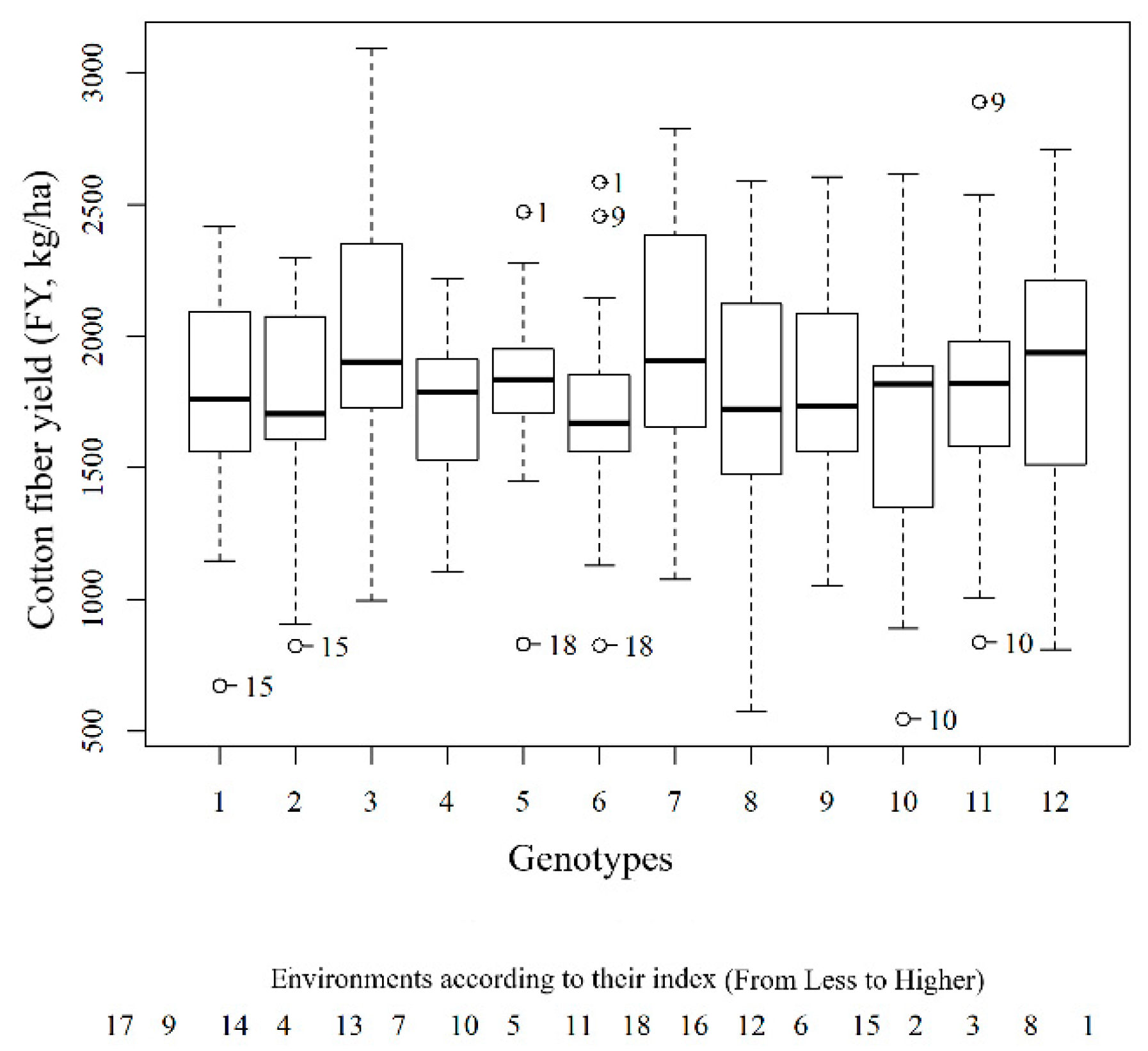
3.1. Analysis of Cotton Yields in Different Environments

The joint analysis of variance for the data of yield of 12 cotton genotypes showed differences (p < 0.05) for environments (E), genotypes (G) and the G × E interaction (Table 2). The significance of the G × E interaction effects indicates the differential performance of genotypes in different environments justifying the use of adaptability and stabilities analysis.

3.2. Potential Influential Points on the Experimental Data

According to the boxplot (Figure 1) in the environments 1, 9, 10, 15 and 18, some genotypes presented phenotypic values that differ significantly from other observations, that is, outliers (Figure 1). The leverage values range from 0.06 to 0.31. The two higher leverage values were observed for environments 1 (0.22) and 17 (0.31) (Figure 1 and Table S1). The further I j is from I ¯ , the larger the leverage is (Figure 1).
The estimates of absolute studentized residuals (SR), DFBETAS and Cook’s distance (CD) range from 0 to 5.03, 0 to 0.21 and from 0 to 1.17, respectively (Tables S1–S3). Considering the environment with leverage values higher than the threshold (0.22), only genotype five (IMA 08 WS) presented values of absolute studentized residuals (2.71) and CD (1.17) higher than the thresholds (2.00 and 1.00), showing that this genotype deserves attention (Tables S1–S3).

3.3. Yield Adaptability and Stability from Experimental Data

The genotypes TMG 41 WS (genotype one), TMG 43 WS (genotype two), BRS 286 (genotype nine) and BRS 368 RF (genotype 11) presented discordant classifications in relation to the parameter of adaptability (Table 3). Specifically, the genotypes one and nine (TMG 41 WS and BRS 286) were characterized as having wide adaptability by Eberhart and Russell and non-parametric regression [11,14] methodologies, and were recommended for unfavorable environments by the quantile regression. Genotype two (TMG 43 WS), recommended for unfavorable environments by Eberhart and Russell and non-parametric regressions, was characterized as having wide adaptability by the quantile regression methodology. Differently from the other methods (non-parametric and quantile regressions), genotype 11 (BRS 368 RF) was considered as having wide adaptability by Eberhart and Russell. Although these genotypes presented discordant classification, according to the defined cutoffs (leverage > 0.22 and SR > 2; DFBETAS > 0.47 or CD > 1), they do not present any influential points (Tables S1–S3 and Figures S1–S4). Therefore, the classification considered is that provided by the Eberhart and Russell methodology. On the other hand, genotype five (IMA 08 WS), that presents a possible influential point at environment 17 (SR = 2.71; CD = 1.17), does not present discordant classification in relation to the parameter of adaptability (Tables S1 and S3). Specifically, this genotype was classified as recommended for unfavorable environments by the three methodologies being studied (Table 3).
Overall, the genotypes present the low stability. The intercept estimated from the Eberhart and Russell method of each genotype (Table 3) is given by the average of the genotypes over environments. On the other hand, non-parametric and quantile regression methodologies use strategies based on the median. The estimated values for the intercept parameter do not present higher differences (Table 3).

3.4. Potential Influential Points in the Synthetic Data

After the insertion of possible influential points at the genotypes 1, 6 and 12, the leverage values ranged from 0.06 (environments 5, 6, 7, 10, 11, 12, 16 and 18) to 0.27 (environment 17) (Table S4).
The estimates of absolute studentized residuals (SR), DFBETAS and Cook’s distance (CD) ranged from 0 to 10.78, 0 to 0.46 and from 0 to 2.04, respectively (Tables S4, S5 and S6). Considering these thresholds (Leverage > 0.22 and SR > 2; DFBETAS > 0.47 or CD > 1), genotypes one (TMG 41 WS), five (IMA 08 WS) and 12 (BRS 369 RF) deserve attention and should be analyzed carefully. According to the used thresholds, genotype six (NUOPAL), which was added an influential point, does not present any problem and can be analyzed considering the Eberhart and Russell classification.

3.5. Yield Adaptability and Stability from Synthetic Data

Among the genotypes that deserve attention, two of them (genotypes 1—TMG 41 WS and 12—BRS 369 RF) correspond to those to which the influential point was added. These genotypes presented discordant classifications in relation to the parameter of adaptability (Table 4). Genotype one (TMG 41 WS) was recommended for unfavorable environments by Eberhart and Russell; it was characterized as having wide adaptability by non-parametric and quantile regression methodologies (Table 4 and Figure S5). On the other hand, genotype 12 (BRS 369 RF) was characterized as having wide adaptability using this method and was recommended for favorable environments by non-parametric and quantile regression methodologies (Table 4 and Figure S6). The recommendation of the other genotypes can consider the Eberhart and Russell results. Genotype six (NUOPAL) was not affected by the “influential point” (Table 4 and Figure S7).
The stability parameter for the genotypes affected by the influential points is defined through R T H 2 or R Q R 0.5 2 for non-parametric and quantile regressions, respectively. Overall, the genotypes where the influential point was added and deserves attention, were classified as having low predictability R T H 2   a n d   R Q R 0.5 2 < 0.70 ) (Table 4). These results agree with those obtained using the Eberhart and Russell methodology, which uses the component of variance from the regression deviations as a measure of stability. The intercept’s estimates presented similar results (Table 4).
In summary, the presence of the influential points underestimates and overestimates the adaptability parameter estimates obtained using Eberhart and Russell, non-parametric and quantile regression methodologies (Table 5).

4. Discussion

In this study, we aimed to evaluate the effect of influential points in methodologies based on regression for adaptability and stability parameter estimation. The Eberhart and Russell [6] methodology, and non-parametric [11,14] and quantile [8,18] regressions were compared. These methodologies are, respectively, based on standard least squares [6] and median (non-parametric and quantile (τ = 0.5) regressions) estimators. In order to do so, a real data set consisting of a yield of 12 early cotton genotypes evaluated in 18 Brazilian Cerrado environments and synthetic data were used.
According to Draper and John [26], an outlier is an observation that provides a large residual. However, an outlier does not necessarily affect the fitted equation, mainly when the outlier presents a low leverage value. To assess the influence of a specific observation in the estimation process, we used some measures to verify the presence of a possible influential point. In the first one, the leverage was used jointly with the studentized residual. The leverage summarizes the potential influence of Y i on all the fitted values according to Fox [21]. The further I j is from I ¯ , the larger the leverage is. In adaptability and stability methods based on regression models, since the independent variable is defined by an environmental index, the environments far away from the mean (zero) can have a considerable impact on the fitted value. Environment 17 (Chapadão do Sul, MS—CHA) presented a leverage value higher than the threshold (0.22) and, therefore, could have impacted the fitted value. However, the leverage presents one issue. A point with high leverage may or may not be influential since the leverage depends only on the independent variable ( I j ). Therefore, another measure is needed to detect an influential point. The studentized residual was used jointly with the leverage for detecting possible influential points, since observations that combine higher leverage with a higher studentized residual exert substantial influence on the regression coefficients. The second one was based on measures direct of the impact on each coefficient through deleting each observation. Nascimento et al. [11] defined the variation, in modulus, between the estimators of the slope coefficient estimated using the methods least squares and using the non-parametric regression method as a measure of the direct influence of one point. Nevertheless, it is usual to scale this measure using the coefficient standard error. The DFBETAS measure the standardized change in regression coefficients. According to Fox [21], values of DFBETAS higher than one or two indicate an influential point. However, since in adaptability and stability studies, the number of environments is small, it is recommended that the size-adjusted threshold proposed by Belsley et al. is used [27] ( 2 number   of   environments ) . Cook’s distance measures the “distance” between the slopes estimated without and with the observation. In general, Cook’s distance was more sensitive compared to the DFBETAS. Differently of the DFBETAS, Cook’s distance was able to detect the inserted influential points. Thus, it is suggested that more than a simple measure is used to assess possible influential points.
After the evaluation of influential points, the analyses of adaptability and stability were performed. Overall, the methodologies based on medians (non-parametric and quantile regressions) were more appropriate in the presence of influential points (synthetic data). These methods are less sensitive in the presence of influential points (as observed in the synthetic data) compared with least square estimators [11,28]. According to John [29], since the median has a bounded influence function, the effect of an outlier on a sample median is bounded, no matter how far the outlying observation is. Therefore, methodologies based on median estimators seem more adequate in the presence of influential points. Nascimento et al. [11] showed that non-parametric regression [14] reduces the influence of influential points resulting from the presence of genotypes with answers to a certain environment that are too different on the estimation of the adaptability parameter. Barroso et al. [8] showed that the quantile regression (τ = 0.5) methodology provides superior results compared to Eberhart and Russell [6] in the presence of influential points.
These results are similar to those obtained in this work. The use of one methodology that is less sensitive to the presence of influential points can avoid misclassification, as it seemed for genotypes 1 and 12 considering the synthetic data. Genotype five, in which was detected by a potential influential point, does not present discordant classification. Thus, in a context of adaptability and stability analysis, only those genotypes that present a discordant classification between methodologies should be analyzed carefully.
Overall, the effect of an influential point in the adaptability parameter can be summarized considering the results obtained for genotypes 1 (TMG 41 WS) and 12 (BRS 369 RF) from the synthetic dataset. Specifically, environments 17 (CHA) and 8 (CV2), respectively, underestimate and overestimate the adaptability parameter estimates obtained using the Eberhart and Russell methodology. However, to identify an influential point is not a simple task. In an adaptability and stability study context, the research should carefully analyze an environment that greatly affects adaptability parameters. To do that, it is interesting to use, in addition to current experience, the measures presented in this manuscript. Regarding the stability parameter, the genotypes do not present higher differences. The intercept estimator from the Eberhart and Russell method of each genotype is given by the average of the genotypes over the environments. On the other hand, non-parametric and quantile regression methodologies use strategies based on the median. Despite it, the estimated values for the intercept parameter do not present higher differences.
Finally, once the recommendation of a genotype is made in a general way for several environments, any methodology that mitigates a differential effect from a specific environment into a genotype seems interesting.

5. Conclusions

The influential points can modify the recommendation of genotypes, based on regression methods, in the presence of a G × E interaction. The non-parametric and quantile (τ = 0.5) regressions based on median estimators are less sensitive to the presence of influential points, avoiding misleading recommendations of genotypes in terms of their adaptability in the presence of influential points. The recommendation of genotypes by the Eberhart and Russell methodology in the presence of an influential point can under or overestimate the adaptability parameter estimates causing a loss of information, time and financial resources. On the other hand, when the dataset does not present any problems related to influential points, the Eberhart and Russell methodology should be used in the genotype classification.

Supplementary Materials

The following are available online at https://www.mdpi.com/article/10.3390/agronomy11112179/s1, Figure S1: Estimated lines by Eberhart and Russell (1966), non-parametric and quantile regressions (τ = 0.50) to the genotype TMG 41 WS, considering the experimental data, Figure S2: Estimated lines by Eberhart and Russell (1966), non-parametric and quantile regressions ( τ = 0.50 ) to the genotype TMG 43 WS, considering the experimental data, Figure S3: Estimated lines by Eberhart and Russell (1966), non-parametric and quantile regressions (τ = 0.50) to the genotype BRS 286, considering the experimental data, Figure S4: Estimated lines by Eberhart and Russell (1966), non-parametric and quantile regressions ( τ = 0.50 ) to the genotype BRS 368 RF, considering the experimental data., Figure S5: Estimated lines by Eberhart and Russell (1966), non-parametric and quantile regressions (τ = 0.50) to the genotype TMG 41 WS, considering the synthetic data, Figure S6: Estimated lines by Eberhart and Russell (1966), non-parametric and quantile regressions (τ = 0.50) to the genotype NUOPAL, considering the synthetic data, Figure S7: Estimated lines by Eberhart and Russell (1966), non-parametric and quantile regressions (τ = 0.50) to the genotype BRS 369 RF, considering the synthetic data, Table S1: Absolute studentized residuals, leverage and environmental index considering the experimental data, Table S2: Difference in adaptability parameter estimated for each genotype with and without the environment (DFBETA) considering the experimental data, Table S3: Cook’s distance for the experimental data, Table S4: Absolute studentized residuals, leverage and environmental index considering the synthetic data, Table S5: Difference in adaptability parameter estimate for each genotype with and without the environment (DFBETA) considering the synthetic data, Table S6: Cook’s distance for the synthetic data.

Author Contributions

Conceptualization, M.N., P.E.T. and I.d.C.S.; formal analysis, M.N., I.d.C.S. and L.M.A.B.; investigation, M.N., L.P.R.T., F.J.C.F. and H.C.A.; methodology, A.C.C.N., M.N., I.d.C.S. and C.F.A.; writing (original draft), M.N., P.E.T. and I.d.C.S.; writing (review and editing), M.N.; P.E.T., I.d.C.S., L.M.A.B., A.C.C.N., C.F.A., L.P.R.T., F.J.C.F., H.C.A. and L.P.d.C. All authors have read and agreed to the published version of the manuscript.

Funding

This research was funded by CAPES, CNPq, FAPEMIG, FUNARBE and FUNDECT (process number 71/019.039/2021).

Institutional Review Board Statement

Not applicable.

Acknowledgments

The authors gratefully acknowledge the the Coordenação de Aperfeiçoamento de Pessoal de Nível Superior (CAPES)—Financial Code 001 and the Conselho Nacional de Desenvolvimento Científico e Tecnológico (CNPq)—Grant number 303767/2020-0 for the financial support.

Conflicts of Interest

The authors declare no conflict of interest.

References

  1. Cruz, C.D.; Regazzi, A.J.; Carneiro, P.C.S. Modelos Biométricos Aplicados ao Melhoramento Genético, 5th ed.; UFV—Universidade Federal de Viçosa: Viçosa, Brazil, 2012; ISBN 9788572694339. [Google Scholar]
  2. Van Eeuwijk, F.A.; Bustos-Korts, D.V.; Malosetti, M. What Should Students in Plant Breeding Know About the Statistical Aspects of Genotype × Environment Interactions? Crop Sci. 2016, 2140, 2119–2140. [Google Scholar] [CrossRef]
  3. Malosetti, M.; Ribaut, J.; Van Eeuwijk, F.A. The statistical analysis of multi-environment data: Modeling genotype-by-environment interaction and its genetic basis. Front. Physiol. 2013, 4, 1–17. [Google Scholar] [CrossRef] [PubMed] [Green Version]
  4. Elias, A.A.; Robbins, K.R.; Doerge, R.W.; Tuinstra, M.R.; Elias, A.A.; Doerge, R.W.; Tuinstra, M.R. Half a Century of Studying Genotype × Environment Interactions in Plant Breeding Experiments. Crop Sci. 2016, 2105, 2090–2105. [Google Scholar] [CrossRef]
  5. Crossa, J.; Vargas, M.; Cossani, C.M.; Alvarado, G.; Burgueño, J.; Mathews, K.L.; Reynolds, M.P. Evaluation and interpretation of interactions. Agron. J. 2015, 107, 736–747. [Google Scholar] [CrossRef] [Green Version]
  6. Eberhart, S.A.; Russell, W.A. Stability Parameters for Comparing Varieties. Crop Sci. 1966, 28, 36–40. [Google Scholar] [CrossRef] [Green Version]
  7. Cruz, C.D.; de Torres, R.A.; Vencovsky, R. An alternative approach to the stability analysis proposed by Silva and Barreto. Revista Brasileira de Genética 1989, 12, 567–580. [Google Scholar]
  8. Mayara, L.; Barroso, A.; Nascimento, M.; Carolina, A.; Nascimento, C. Metodologia para análise de adaptabilidade e estabilidade por meio de regressão quantílica. Pesquisa Agropecuária Brasileira 2015, 50, 290–297. [Google Scholar] [CrossRef] [Green Version]
  9. Barroso, L.M.A.; Nascimento, M.; Barili, L.D.; Nascimento, A.C.C.; do Vale, N.M.; e Silva, F.F.; de Carneiro, J.E.S. Analysis of the adaptability of black bean cultivars by means of quantile regression. Ciência Rural 2019, 49, e20180045. [Google Scholar] [CrossRef]
  10. Lin, C.S.; Binns, M.R. A Superiority Measure of Cultivar Performance for Cultivar × Location Data. Can. J. Plant Sci. 1988, 68, 193–198. [Google Scholar] [CrossRef]
  11. Nascimento, M.; Ferreira, A.; Ferrão, R.G.; Campana, A.C.M.; Bhering, L.L.; Cruz, C.D.; Ferrão, M.A.G.; da Fonseca, A.F.A. Adaptabilidade e estabilidade via regressão não paramétrica em genótipos de café. Pesquisa Agropecuaria Brasileira 2010, 45, 41–48. [Google Scholar] [CrossRef] [Green Version]
  12. Nascimento, M.; Cruz, C.D.; Campana, A.C.M.; Tomaz, R.S.; Salgado, C.C.; de Paula Ferreira, R. Alteração no método centroide de avaliação da adaptabilidade genotípica. Pesquisa Agropecuaria Brasileira 2009, 44, 263–269. [Google Scholar] [CrossRef] [Green Version]
  13. Nascimento, M.; Ferreira, A.; Campana, A.C.M.; Salgado, C.C.; Cruz, C.D. Multiple centroid methodology to analyze genotype adaptability. Crop Breed. Appl. Biotechnol. 2009, 9, 8–16. [Google Scholar] [CrossRef] [Green Version]
  14. Theil, H. A Rank Invariant Method of Linear and Polynomial Regression Analysis. Indag. Math. 1950, 23, 85–91. [Google Scholar]
  15. Children, N.; Kries, V.; Ness, A.R.; Ong, K.K.; Beyerlein, A. Genetic Markers of Obesity Risk: Stronger Associations with Body Composition in Overweight Compared to Normal-Weight Children. PLoS ONE 2011, 6, 4–7. [Google Scholar] [CrossRef] [Green Version]
  16. Barroso, L.M.A.; Nascimento, M.; Nascimento, A.C.C.; Silva, F.F.; Serão, N.V.L.; Cruz, C.D.; Resende, M.D.V. Regularized quantile regression for SNP marker estimation of pig growth curves. J. Anim. Sci. Biotechnol. 2017, 8, 1–9. [Google Scholar] [CrossRef] [Green Version]
  17. Nascimento, A.C.C.; de Lima, J.E.; Braga, M.J.; Nascimento, M.; Gomes, A.P. Eficiência técnica da atividade leiteira em Minas Gerais: Uma aplicação de regressão quantílica. Rev. Bras. Zootec. 2012, 41, 783–789. [Google Scholar] [CrossRef] [Green Version]
  18. Koenker, R.; Bassett, G. Regression Quantiles. Econometrica 1978, 46, 33–50. [Google Scholar] [CrossRef]
  19. Tukey, J.W. Exploratory Data Analysis; Addison-Wesley: Reading, MA, USA, 1977; Volume 2. [Google Scholar]
  20. Chatterjee, S. Sensitivity Analysis in Linear Regression. Wiley Ser. Probab. Math. Stat. 1989, 38, 138. [Google Scholar] [CrossRef]
  21. Fox, J. Generalized Linear Models. Appl. Regres. Anal. Gen. Linear Model. 2008, 135, 379–424. [Google Scholar] [CrossRef]
  22. R Core Team. R: A Language and Environment for Statistical Computing; R Core Team: Vienna, Austria, 2020. [Google Scholar]
  23. Komsta, L. mblm: Median-Based Linear Models. Available online: https://cran.r-project.org/web/packages/mblm/index.html (accessed on 10 January 2021).
  24. Koenker, R.; Portnoy, S.; Ng, P.T.; Zeileis, A.; Grosjean, P.; Ripley, B.D. quantreg: Quantile Regression. Available online: https://cran.r-project.org/web/packages/quantreg/index.html (accessed on 1 January 2021).
  25. Cruz, C.D. Acta Scientiarum GENES—A software package for analysis in experimental statistics and quantitative genetics. Acta Scientiarum Agron. 2013, 35, 271–276. [Google Scholar] [CrossRef]
  26. Draper, N.R.; John, J.A. Influential observations and outliers in regression. Technometrics 1981, 23, 21–26. [Google Scholar] [CrossRef]
  27. Belsley, D.A.; Kuh, E.; Welsch, R.E. Regression Diagnostics: Identifying Influential Data and Sources of Collinearity; Wiley: New York, NY, USA, 1980; ISBN 0471058564. [Google Scholar]
  28. Sprent, P.; Smeeton, N.C. Applied Nonparametric Statistical Methods, 4th ed.; CRC Press: Boca Raton, FL, USA, 2007; ISBN 13978-1-58488-701-0. [Google Scholar]
  29. John, O. Robustness of Quantile Regression to Outliers. Am. J. Appl. Math. Stat. 2015, 3, 86–88. [Google Scholar] [CrossRef]
Figure 1. Boxplot of yield of 12 early cotton genotypes evaluated in each one of 18 Brazilian Cerrado environments. Genotypes—1: TMG 41 WS; 2: TMG 43 WS; 3: IMA CV 690; 4: IMA B2RF; 5: IMA 08 WS; 6: NUOPAL; 7: DP 555 BGRR; 8: DELTA OPAL; 9: BRS 286; 10: BRS 335; 11: BRS 368 RF; 12: BRS 369 RF. Environments—1: TRI; 2: SHE1; 3: SHE2; 4: PVA1; 5: PVA2; 6: PVA3; 7: CV1; 8: CV2; 9: SIN; 10: PPA1; 11: PPA2; 12: LEM; 13: SDES; 14: MON; 15: MAG; 1616: TER; 17: CHA; 18: SORT.
Agronomy 11 02179 g001
Table 1. Abbreviations of genotypes and description of environments regarding geographic coordinates and climatic characteristics of cotton variety test sites evaluated for environmental impact in the Brazilian Cerrado.
Environment State Abbr.SeasonAlt.Lat.Long.Prec.Temp.
m° SWmm°C
Trindade, MG1—TRI2013–201492721.0644.188026.2
Santa Helena de Goiás, GO2—SHE12013–201456217.4850.3566127.1
3—SHE22014–2015 64226.8
Primavera do Leste, MT4—PVA12013–201446515.3354.1760127.5
5—PVA32014–2015 62526.9
6—PVA42014–2015 63826.9
Campo Verde, MT7—CV12013–201473615.3255.186425.8
8—CV22014–2015 87925.4
Sinop, MT9—SIN2013–201434511.5155.340930.9
Pedra Preta, MT10—PPA12013–201424816.3754.2884926
11—PPA22014–2015 84026.2
Luís Eduardo Magalhães, BA12—LEM2013–201476912.545.4780225.4
São Desidério, BA13—SDES2013–201449712.2144.5865827
Magalhães de Almeida, MA14—MON2013–201482117.2651.145530.1
Montividiu, GO15—MAG2013–2014363.2342.1281726.8
Teresina, PI16—TER2013–2014725.0542.4881026.8
Chapadão do Sul, MS17—CHA2014–201580018.4752.3789826.7
Sorriso, MT18—SOR2014–201536512.3255.4243631.2
Data obtained from the National Institute of Meteorology (INPE). State abbreviations: MG, Minas Gerais; GO, Goiás; MT, Mato Grosso; BA, Bahia; MA, Maranhão; PI, Piauí; MS, Mato Grosso do Sul.
Table 2. Joint analysis for yield of 12 early cotton genotypes evaluated in 18 Brazilian Cerrado environments in the 2013–2014 and 2014–2015 cropping seasons.
Source of VariationDegree of FreedomMean Square
Environments (E)177,723,577.00 *
Blocks/environment5444,347.00
Genotypes (G)11797,936.00 *
G × E187201,748.00 *
Residual59424,059.00
General average 1810.28
CV (%) 13.29
* Significant at the 0.05 probability level. CV = coefficient of variation.
Table 3. Estimate of adaptability and stability parameters by the Eberhart and Russell (1966), non-parametric and quantile regression methodologies of yield of 12 early cotton genotypes (experimental data).
Genotype β ^ 0 E R β ^ 0 T H β ^ 0 Q R 0.5 β ^ 1 E R β ^ 1 T H β ^ 1 Q R 0.5 R E R 2 R T H 2 R Q R 0.5 2 σ d i E R 2
TMG 41 WS1763.611756.781770.100.930.940.87 *74.7074.6854.2543,575.10 *
TMG 43 WS1732.821670.221690.160.80 *0.74 *0.9565.8165.5241.2950,291.91 *
IMA CV 6902027.642007.152015.171.17 *1.14 *1.10 *85.8085.7558.6632,384.43 *
IMA B2RF1737.201744.051732.980.62 *0.69 *0.60 *67.8166.9843.8525,088.63 *
IMA 08 WS1818.911822.951832.940.61 *0.51 *0.67 *50.2148.7119.0257,350.26 *
NUOPAL1698.351677.301693.740.970.981.0484.4484.4261.6623,602.33 *
DP 555 BGRR1978.411970.501961.591.22 *1.28 *1.15 *92.9192.7072.5313,319.51 *
DELTA OPAL1710.321724.101712.431.21 *1.15 *1.11 *86.2786.0566.0833,798.50 *
BRS 2861801.361817.321806.780.980.970.90 *81.3881.3858.5231,188.39 *
BRS 3351743.391807.281802.791.15 *1.11 *1.10 *77.8077.7055.0058,799.79 *
BRS 368 RF1827.351843.901833.291.14 *1.050.9983.5083.0558.6737,968.09 *
BRS 369 RF1883.991864.511862.171.22 *1.27 *1.26 *92.2692.1072.7615,247.75 *
* Significant at the 0.05 probability level; β ^ 0 E R : intercept of Eberhart and Russell [6] method (based on standard least squares); β ^ 0 T H   a n d   β ^ 1 T H : intercept and parameter of adaptability of Non-parametric Regression [11,14] method; β ^ 0 Q R 0.5 : intercept of Quantile Regression [8,24] method; β ^ 1 E R : parameter of adaptability using the Eberhart and Russell [6] method; β ^ 1 T H : parameter of adaptability using the Non-parametric Regression [11,14] method; β ^ 1 Q R 0.5 : parameter of adaptability using the Quantile Regression [8,18] method; R E R 2   :   coefficient of determination using the Eberhart and Russell [6] method; R T H 2 : coefficient of determination using the Non-parametric Regression [11,14] method; R Q R 0.5 2 : coefficient of determination using the Quantile Regression [8,18] method; σ d i E R 2 : regression deviation using the Eberhart and Russell [6] method.
Table 4. Estimate of adaptability and stability parameters by the Eberhart and Russell (1966), non-parametric and quantile regression methodologies of yield of 12 early cotton genotypes (synthetic data).
Genotype β ^ 0 E R β ^ 0 T H β ^ 0 Q R 0.5 β ^ 1 E R β ^ 1 T H β ^ 1 Q R 0.5 R E R 2 R T H 2 R Q R 0.5 2 σ d i E R 2
TMG 41 WS1842.151733.051733.050.57 *0.990.9924.1813.960.33149,394.43 *
TMG 43 WS1732.821694.231688.770.84 *0.83 *0.9564.6464.550.4152,273.67 *
IMA CV 6902027.652049.112042.811.20 *1.17 *1.24 *81.6781.420.5643,647.29 *
IMA B2RF1737.201745.811760.930.68 *0.73 *0.65 *72.0671.640.4621,048.02 *
IMA 08 WS1818.911823.001833.220.63 *0.50 *0.68 *48.2645.000.1659,890.85 *
NUOPAL1747.641711.141697.451.041.081.21 *71.2171.180.5561,413.14 *
DP 555 BGRR1978.421989.741970.031.28 *1.33 *1.25 *92.2892.030.7615,099.32 *
DELTA OPAL1710.331706.011712.891.29 *1.27 *1.12 *88.2488.140.6428,150.74 *
BRS 2861801.361819.521815.061.011.14 *1.0678.6278.420.5836,778.73 *
BRS 3351743.391768.411785.991.22 *1.18 *1.26 *77.7777.670.5358,952.44 *
BRS 368 RF1827.351833.401842.311.19 *1.16 *1.0581.3380.780.5843,821.64 *
BRS 369 RF1805.581866.881862.691.031.28 *1.26 *50.7946.730.51151,289.81 *
* Significant at the 0.05 probability level; β ^ 0 E R : intercept of Eberhart and Russell [6] method; β ^ 0 T H   a n d   β ^ 1 T H : intercept and parameter of adaptability of Non-parametric Regression [11,14] method; β ^ 0 Q R 0.5 : intercept of Quantile Regression [8,18] method; β ^ 1 E R : parameter of adaptability using the Eberhart and Russell [6] method; β ^ 1 T H : parameter of adaptability using the Non-parametric Regression [11,14] method; β ^ 1 Q R 0.5 : parameter of adaptability using the Quantile Regression [8,18] method; R E R 2   :   coefficient of determination using the Eberhart and Russell [6] method; R T H 2 : coefficient of determination using the Non-parametric Regression [11,14] method; R Q R 0.5 2 : coefficient of determination using the Quantile Regression [8,18] method; σ d i E R 2 : regression deviation using the Eberhart and Russell [6] method.
Table 5. Summary of changes in the classification in relation to the parameter of adaptability obtained using the Eberhart and Russell (1966), non-parametric and quantile Regression methodologies for three early cotton genotypes that deserves attention and should be analyzed carefully according to the measures used to assess influential points.
DatasetGenotypeEberhart and RussellNon-ParametricQuantile
SyntheticTMG 41 WSUnfavorableGeneralGeneral
IMA 08 WSUnfavorableUnfavorableUnfavorable
BRS 369 RFGeneralFavorableFavorable
ExperimentalIMA 08 WSUnfavorableUnfavorableUnfavorable
Publisher’s Note: MDPI stays neutral with regard to jurisdictional claims in published maps and institutional affiliations.

