Comparative Analysis of Energy and GHG Emissions Using Fixed and Variable Fertilization Rates

Abstract

Reducing the overuse of mineral fertilizers in crop production is a key factor related to healthier soil, healthier food, and more economical, efficient, and cleaner agricultural production. The aim of this study was to investigate and to compare the effects of fixed and variable rate fertilization with fertilizer consumption, energy consumption, and environmental impact. A 4-year experimental field study using crop rotation of four plants (spring barley, winter oilseed rape, winter wheat, and faba bean) was performed. Fertilization with phosphorus and potassium at a variable rate were performed and applied based on the soil properties analyzed before the start of the research and completion of the fertilization maps. Nitrogen fertilization was performed by additional fertilization using a proximal N-sensor, which gives the accurate nitrogen uptake in plants in real-time. This was followed by a comparative evaluation analysis of variables and conventional fixed-rate fertilization methods to assess fertilizer consumption, energy consumption, environmental impact, and economic efficiency. The results of the study showed that an application of a variable fertilization rate can reduce the total amount of nitrogen, phosphorus, and potassium fertilizers by 24.9%, energy consumption by 3463.1 kg ha⁻¹, and emissions of greenhouse gases (GHG) by 341.5 kg CO_2eq ha⁻¹ compared to fixed fertilization rate. The method of fertilization with a variable application rate reduced the costs of fertilization, and at the same time, the costs of the total plant production by €168.0 ha⁻¹, on average.

1. Introduction

Plant nutrition is one of the most important factors on which the yield and the quality of agricultural products depend [1]. Therefore, organic and mineral fertilizers are used to enrich the soil with nutrients and to achieve the highest soil fertility. Over the last few decades, fertilizer use has been growing exponentially around the world. In 2018, global consumption of chemical and mineral fertilizers amounted to 188 million tons, of which nitrogen (N) averaged 58%, phosphorus (P₂O₅) 22%, and potassium (K₂O) 21%. In a period of 18 years (2000–2018), fertilizers’ consumption increased by about 40% [2]. In Europe, fertilizers per crop area increased by 10% during this period and reached 77 kg ha⁻¹, N–49, P₂O₅–13, and K₂O–15 kg ha⁻¹, respectively [2]. Intensive use of mineral fertilizers and application of conventional fertilization methods have negative effects on the soil, the environment, and human health. For example, ammonia emission from over-fertilized lands can damage organisms living in lakes and reservoirs, and the amount of nitrate concentration in drinking water can increase as well. Excessive amounts of fertilizers are related to higher GHG emissions [1,3]. Traditionally, fertilizers are applied to all arable land, regardless of soil variation in the field area [4]. Variable rate fertilization (VRF) is essential for the implementation of precision farming and for the efficient use of mineral fertilizers and nutrient management in plants adapted to the conditions of individual field sites [5]. It should be taken into consideration that the application of VRF usually requires prior knowledge of the field characteristics. This method often relies on accurate soil sampling and/or monitoring and analysis of crop yields for a specific field site [6].

The most important aim of precision agriculture is to adapt agricultural technological processes to the conditions of individual field locations. Precision farming can be defined as the longitudinal experience of farmers in order to ensure the sustainability of agriculture, based on four eligibility criteria: Application of the right method, the right rate of materials, the right choice of time, and the right application place [3,7,8,9].

Precision agriculture and VRF are closely linked to smart digital technologies such as Global Navigation Satellite Systems (GNSS), Remote Sensing (RS), Geographic Information Systems (GIS), crop or soil mapping tools, machine learning, and remote and proximal sensors capable of measuring and predicting crop and soil properties in real-time [3,5,10,11,12,13,14].

Agriculture is one of the economic sectors influencing climate change and directly or indirectly causing greenhouse gas (GHG) emissions. The agricultural sector is responsible for approximately 25% of CO₂, 50% of CH_4, and 70% of N₂O emissions worldwide. It contributes to approximately 13.5% of total anthropogenic GHG emissions [15,16]. Nitrous oxide (N₂O) is a major product of GHG in intensive agriculture [17]. The concentration of N₂O has a 310 times higher warming potential than CO₂. The aim of agricultural management is to apply less N fertilizers without decreasing crop yields and to reduce N₂O emissions and nitrate leaching from agriculture, and minimizing the negative impact for the environment [18]. The abundant use of N fertilizers increases the yield, but the application efficiency remains low. It can lead to environmental problems related to nitrate leaching and atmosphere pollution with nitrous oxide [19]. Only up to 50% of synthetic N fertilizers applied in agriculture in the US are assimilated by plants, and the rest is leached from the soil as NO₃, causing surface and groundwater pollution, or emitted to the atmosphere as NH₃, N₂, or N₂O [20]. Rogovska et al. [20] claimed that accurate nitrogen fertilizer management can improve the efficiency of N fertilizer use while reducing farmers’ costs and the environmental impact of crop production. The application of precision agricultural technologies can contribute to the reduction of GHG emissions, have a positive impact on farm productivity, and the economy [16]. Nawar et al. [21] conducted a review of different soil nutrient management zones for variable fertilization and found that the application of such methods is much more efficient and has a lower environmental impact compared to traditional fixed rate application methods. The authors note that there is not enough information in the agricultural studies regarding the cost-benefit analysis of VRF application based on management zones compared to fixed rate fertilization.

Remote (satellites, drones) and proximal (Green Seeker, Crop Circle, Crop Spec) sensing of crop to determine N nutrient status were presented by Tremblay [22], and handheld sensors Dualex Scientific^TM (FORCE-A, Orsay, France), SPAD (Konica Minolta, Tokyo, Japan) that were used to evaluate N demand were described by Ferguson [23]. Burton et al. [24] investigated the use of different types of optic sensors Vis-IR, ATRand Raman spectroscopy (CRAIC Technologies, San Dimas, USA) to measure soil chemical properties in the field. Saiz-Rubio and Rovira-Mas [25] reviewed the current state of advanced farm management systems, reviewing each essential step, from data collection in crop fields to the application of a variable rate to enable growers to make optimal decisions while saving money and protecting the environment.

The research on precision fertilization with variable rate application can already be found in agricultural journals: Utilization of variable rate nitrogen to improve nitrogen use efficiency [18], application and economic assessment of variable rate fertilizer in wheat [4], phosphorus and potassium precision fertilization [26]. However, a comprehensive analysis of fertilizer demand, energy, economic, and environmental impact of different fertilization methods using long-term crop rotation is still lacking. The aim of this work was to investigate and to compare the effects of two fertilization methods, i.e., fixed rate used in conventional farming practice and variable rate, applied after analyzing the soil and assessing the changes in fertilizer consumption, energy consumption, GHG emissions, and economic costs related to fertilizers.

2. Materials and Methods

2.1. Experiment Site and Design

Field experimental studies were conducted in 2015–2019 in the northern part of Lithuania (56°10.109′ N, 23°39.9848′ E), on a farm in the Joniškis district (Figure 1). The crops were grown according to the following crop rotation: Spring barley (Hordeum vulgare L.) variety Propino (2016, seeding time 8 April 2016), winter oilseed rape (Brassica napus L.) variety Visby (2017, 28 August 2016), winter wheat (Triticum aestivum L.) variety Skagen (2018, 30 August 2017), and faba beans (Vicia faba L.) variety Fuego (2019, 8 April 2019). The soil was described as sandy to silty loam according to the soil granulometric classification [27]. Experimental studies were performed comparing 2 different fertilization methods. The fixed fertilization rate (FRF) was determined using the recommended fertilizer rates based on the assumed yield for each crop. The variable fertilization rate (VRF) was determined based on soil characteristics in site-specific areas, crop assumed yield, and nutrient requirements for each crop.

Average (2016–2019) annual precipitation was 505.7 mm, and the average annual air temperature was +8.0 °C (meteo.lt). During plant vegetation in July 2018, the highest average monthly temperature of +20.8 °C was recorded. The lowest temperature −7.7 °C was observed in January 2016. The driest year was 2018, and the wettest year 2016. The dynamics of temperature and precipitation in 2016–2019 is shown in Figure 2.

Field boundaries were measured on 16 September 2015, with an off-road vehicle Toyota Hilux (Toyota Motor Corporation, Toyota, Japan). The total field size was determined to be 11.37 ha by using the GPS coordinate positioning equipment Trimble EZ-Guide 250 with GPS antenna (Trimble Navigation Ltd., Alpharetta, GA, USA). John Deere 6630 tractor (John Deere GmbH & Co., Mannheim, Germany), spreader Rauch Axis-H (Rauch Landmaschinenfabrik GmbH, Sinzheim, Germany), Rauch spreader terminal CCI 100 (Müller GmbH, Rheinfelden, Germany) were used to spread the fertilizer according to variable rate fertilization maps. The crop was harvested with a John Deere S685 harvester (John Deere GmbH & Co.KG, Zweibrücken, Germany) with a working width of 9.14 m.

2.2. Measurements of Soil Electrical Conductivity, Field Subdivision, and Soil Sampling

Prior to the start of the experiment, soil apparent electrical conductivity (ECa) was measured using an EM-38 MK-2 (Geonics Ltd., Mississauga, Canada) at a depth of 0–1.5 m in the vertical position to determine differences in the field soil’s properties and to establish an accurate soil sampling plan. EM-38 readings were applied while driving a Toyota off-road vehicle towing EM38-MK2 mounted on plastic sledges at a speed of 10–15 km h⁻¹ in parallel technological tracks, separated by 30 m, with a total of 1046 readings (92 readings ha⁻¹) for the field of 11.37 ha. These readings were stored on a computer Panasonic Toughbook CF 19 (Panasonic Corporation, Osaka, Japan).

ECa readings were converted to a CSV file format using Convert EM38-MK2 software, and subsequently, an ECa map (Figure 3) was created using the Open Source Geographic Information System (QGIS) program. A total of 4 areas (each approximately 3 ha) with different ranges of ECa were delineated (Figure 1). The delineated plots in a digital shape (SHP) file was sent back to the field computer, and soil samples were taken.

Soil (at a depth of 20–30 cm) was sampled on 17 September 2015 and 2 September 2019 using an automatic soil sampling equipment (Figure 4) developed by Agricon (GmbH, Jahna, Germany) and manufactured by Adigo AS, Langhus, Norway). The subsamples were collected while driving non-stop (50% more efficient than sampling at a stop [28]) in the trajectory of the letter Z and combined in one sample in each of the 4 homogeneous areas delineated previously.

Four samples were taken from 4 areas formed according to soil ECa differences. One sample consisted of 15–20 subsamples (Figure 1). These samples were collected into boxes containing 300–500 g of soil. After all the boxes were filled, soil samples from each box were placed into separate plastic bags, and labeled with a bar code including information, such as the coordinates, date, and time of sampling. Samples were sent to an accredited laboratory Agrolab GmbH (Leinefelde-Worbis, Germany), where their granulometric structure, magnesium (Mg) and pH (CaCl₂ method), potassium (K) and phosphorous (P) (CAL method) were determined.

2.3. Determination of Fixed and Variable Fertilization Rates for Phosphorus and Potassium

In order to apply the fertilizer at a variable rate, fertilization plans were drawn up (Figure 5). Results of the soil analysis were imported into an agronomic software Agriport. Then, variable fertilizer application rates for a 4-year crop rotation were calculated using the data from soil analysis, the uptake of nutrients P and K for each crop and its assumed yield (t ha⁻¹), respectively: Spring barley (7 t ha⁻¹) P₂O₅–33 kg ha⁻¹, K₂O–25.7 kg ha⁻¹; winter rape (5 t ha⁻¹) P₂O₅–33 kg ha⁻¹, K₂O–25.7 kg ha⁻¹; winter wheat (8 t ha⁻¹) P₂O₅–33 kg ha⁻¹, K₂O–25.7 kg ha⁻¹; faba beans (4 t ha⁻¹) P₂O₅–33 kg ha⁻¹, K₂O–25.7 kg ha⁻¹. The maps for P and K fertilization for the computer of Rauch spreader were created in a SHP file also using Agriport online program. In order to generate a variable rate fertilization (VRF) map for each element, soil analysis was loaded into the program. Then, crop rotation and assumed yield of each crop were entered into the program, which automatically generated VRF maps for each fertilizer. Fertilizers P and K were spread at a variable rate according to the fertilization map, distributing 25% of the planned 4-year fertilization rate in each year. Magnesium was enough to satisfy crop demand in the whole rotation and was not applied.

Fixed rates of fertilization (FRF) for nutrients P and K were calculated using the data from the agronomic software Agriport only for nutrient uptake for each crop and assumed yield, respectively: For spring barley (7 t ha⁻¹) P₂O₅–56 kg ha⁻¹, K₂O–42 kg ha⁻¹; for winter rape (5 t ha⁻¹) P₂O₅–89.3 kg ha⁻¹, K₂O–49.8 kg ha⁻¹; for winter wheat (8 t ha⁻¹) P₂O₅–64 kg ha⁻¹, K₂O–48 kg ha⁻¹; for faba beans (4 t ha⁻¹) P₂O₅–47.6 kg ha⁻¹, K₂O–56 kg ha⁻¹.

2.4. Yara N-Sensor ALS Calibration

Before starting to fertilize winter wheat in the field, a manual proximal sensor Yara N-tester (manufactured by Konica Minolta INC, Japan with Yara software) was used to calibrate the proximal Yara N-Sensor ALS (manufactured by Tec5 GmbH, Germany and developed by Yara International ASA, Oslo, Norway). Calibration was needed to set the N application rate for the Skagen variety of winter wheat at certain growth stages (BBCH 30; 37) in a repeatable part of the field. Yara N-Sensor ALS can collect data only to determine N uptake in the crop and cannot recommend N application rate. An N-tester helps to determine N optimum application rate for different wheat varieties. The calibration location for the device was selected after a visual assessment of the winter wheat field after entering the 4th technological track from the field edge. Measurements were performed by randomly selecting the middle part of the fully developed last leaves of 30 different plants in the 20 m technological track section (Figure 6). The area measured with the N-tester was scanned with Yara N-Sensor ALS device to complete the calibration process. Then, the N application rate for the winter wheat was entered into the terminal using the N application program in the tractor and this software adjusted the N rate in site-specific areas in real-time while driving in the field.

2.5. Fixed and Variable Rate Application for Nitrogen Fertilization

The FRF method was not performed in the field as an actual comparison. FRF for N nutrient was calculated based on conventional farming experience for spring barley N–50 kg ha⁻¹, winter oilseed rape N–188 kg ha⁻¹, winter wheat N–210 kg ha⁻¹, and faba beans N–70.2 kg ha⁻¹, respectively. For the first N application for winter wheat N–40 kg ha⁻¹ (BBCH 23), and for winter oilseed rape N–60 kg ha⁻¹ (BBCH 18), fixed rates were calculated based on conventional farming experience also when using VRF method. For the first N application, it was not possible to use the Yara N-Sensor ALS since it could not collect data from the poor biomass of the crops. For spring barley and faba beans, fixed N nutrient rates were calculated according to conventional farming experience and applied only once before seeding using a fixed rate.

VRF additional application was made only 2 times at different growth stages: For winter wheat N–84 kg ha⁻¹ (BBCH 30) and N–75 kg ha⁻¹ (BBCH 37); for winter oilseed rape N–72 kg ha⁻¹ (BBCH 25) and N–43 kg ha⁻¹ (BBCH 41).

Yara N-Sensor ALS agronomic software calculated the actual N-uptake of the crop. Using N application software optimum rates for VRF in site-specific areas were derived from the N-uptake data in the crop. Calculated rates were sent to the spreader controller, which adjusted the shutters of the implement. At that time, the N-sensor was installed on the roof of the tractor, scanning the crop in 4 m stripes on both sides when driving at 30 m width tramlines.

Information about the fertilizers applied and the amount of N absorbed by the plants in individual parts of the field was transmitted online from the computer inside the tractor to the Agriport program into the office computer. Fertilizer rates for each part of the field and an average could be seen in this program. In our case, N fertilizers YaraBela AXAN NS 27–4 and YaraBela SULFAN NS 24–6 were applied at an average variable rate: For oilseed rape (2017) N–72 kg ha⁻¹ (300 kg ha⁻¹ YaraBela SULFAN) at BBCH 25 and N–43 kg ha⁻¹ (179 kg ha⁻¹ YaraBela SULFAN) at BBCH 41 growth stages; for winter wheat (2018) N–84 kg ha⁻¹ (311 kg ha⁻¹ YaraBela AXAN) at BBCH 30 and N–75 kg ha⁻¹ (278 kg ha⁻¹ YaraBela AXAN) at BBCH 37 growth stages.

2.6. Assessment of Energy Use and GHG Emissions

Fertilizer energy consumption (MJ ha⁻¹) using variable rate fertilization (VRF) and fixed rate fertilization (FRF) was calculated by multiplying the amount of fertilizer used by the energy equivalent the N fertilizer (60.6 MJ kg⁻¹) [29]. Energy consumption equivalents for P₂O₅ and K₂O are presented in

Table 1. Equivalents of energy consumption and GHG emissions for basic fertilizers [29,30].

Fertilizers	Energy Equivalent (MJ kg−1)	GHG Emission Equivalent (kg CO2eq kg−1)
N	60.6	4.96
P2O5	11.1	1.35
K2O	6.7	0.58

. In order to compare fertilization methods, the difference in energy consumption between VRF and FRF was calculated. Another very important benchmark that has been identified was the reduction of fertilizers energy consumption per ton of crop. Fixed and variable fertilizer rates were calculated for an assumed average yield using yield historical data in this field from the last 4 years for each crop: 7.0 t ha⁻¹ for spring barley; 5.0 t ha⁻¹ for winter oilseed rape; 8.0 t ha⁻¹ for winter wheat; 4.0 t ha⁻¹ for faba beans. Therefore, such yields were used in further calculations. In this field, the last historical yields were received using a fixed application rate based only on nutrient uptake with the yield. For our study, it was important in 4 year crop rotation to get the same yield with a lower application rate, which was based not only on nutrient uptake with the yield but also using data about nutrient stocks in the soil. In the farming business, the main goal should be to get more profit, but not the highest yields. This can be achieved using modern precision farming technologies like VRF.

The environmental impact assessment identified GHG emissions (kg CO_2eq ha⁻¹) from different VRF and FRF fertilization methods. GHG emissions were calculated by multiplying the amount of fertilizer used for each method by the GHG equivalents (kg CO_2eq kg⁻¹) given in Table 1. According to Lal et al. [29,30], the CO₂ emission equivalent per kilogram of N fertilizers was 4.96, for P₂O₅ and K₂O were 1.35 and 0.58 kg CO₂ kg⁻¹, respectively. The difference in GHG emissions for each fertilizer type between VRF and FRF methods was also calculated. In order to assess the environmental impact of different fertilization methods, the reduction of GHG emissions per ton of crop yield was calculated based on yield (for spring barley, winter oilseed rape, winter wheat, and faba beans 7.0, 5.0, 8.0, 4.0 t ha⁻¹, respectively).

2.7. Statistical Analysis

To ensure the statistical reliability of the data, the soil properties and yield studies of each crop were performed in 4 replicates of random samples. Each soil sample consisted of randomized 15–20 subsamples. Experimental study data were processed using one-way analysis of variance program ANOVA. The data was evaluated by calculating the smallest significant difference with the level of statistical significance (p < 0.05) using Tukey’s HSD method [31,32]. The different letters in

Table 2. Analysis of soil properties at the beginning of 2015 and at the end of 2019.

Sample No.	Element pH		Element P mg 100 g−1 Soil		Element K mg 100 g−1 Soil		Element Mg mg 100 g−1 Soil		Structure and Soil Group
	2015	2019	2015	2019	2015	2019	2015	2019	2015	2019
1	7.4a	7.4a	9.1a	7.9e	16.4a	9.9e	14.4a	14.1a	sL/4
2	7.2a	7.3a	17.5b	16.6b	23.9b	14.0f	18.7b	19.6b	sL/4
3	7.2a	7.1a	6.6c	8.2ef	11.5c	8.4g	15.3a	16.5d	sL/4
4	7.1a	7.2a	59.9d	48.5g	41.3d	27.6h	23.9c	23.5c	sL/4
Average	7.2	7.3	23.2	20.3	23.3	15.0	18.1	18.4	sL/4
Recommended interval for optimum nutrient amount *	6.3–7.0		4.9–7.2		11.0–16.0		7.6–11.0		-

Notes: Soil group sL/4 means sandy light loam, clay particles (<0.002 mm) >17–25%, fine soil fractions (<0.006 mm) >23–35% [27]. Sample No. 4 was particularly different from other samples because this sampling area was close to the pig complex (Figure 1). * Recommended interval means the optimum nutrient amount available for the most row crops in the soil according to its granulometric structure and soil group. The different letters indicate the significant difference between the values.

indicate the significant difference between the values.

3. Results and Discussion

3.1. Soil Analysis

At the beginning of the research in 2015, the average of each element level in analyzed soil samples was above the optimum level (Table 2). At the end of the studies in 2019, the average K element concentration in the re-analyzed soil samples was reduced significantly (35.6%) to the optimum level, but the rest of the elements stayed above. The main reason for K element reduction was due to the sampling area No. 3 because of higher biomass and yield. Increasing yield leads to higher K element uptake. Phosphorus concentration in all samples in the soil was in or above the optimum level. The highest concentration for elements P and K was found in sample No. 4.

Mg and pH levels in all samples were above the optimum level at the beginning and at the end of the study.

The amount of elements in the soil changed in all the samples throughout the 4-year period: pH increased on average by 1.4%, Mg increase–1.7%, P decreased–12.5%, K decreased–35.6%, respectively (Figure 7). Results received from the laboratory were imported into agronomic software Agriport. All nutrient distribution maps were generated automatically using this program. Agriport has algorithms, which helps to interpolate the spaces between the different sampling areas with different soil sample results. This feature helps to get a better visual view of the nutrient distribution in the field.

Analogous studies by Kulczycki and Grocholski [26] at the start of experimental field research found very high levels of potassium in the soil, and the element potassium exceeded the recommended levels of 82% of the total area. After six years of potassium fertilization at a variable rate, marked changes were observed—38% of the total field area was already attributed to the optimal element content in the soil, and very high potassium levels were found in only 18% of the field area. Meanwhile, the variable rate of phosphorus fertilization increased the field area with a low P element level by 9% and the medium element level by 6%, but the field area with a high P element level decreased by 7%, and the very high P element level decreased by 8%, respectively.

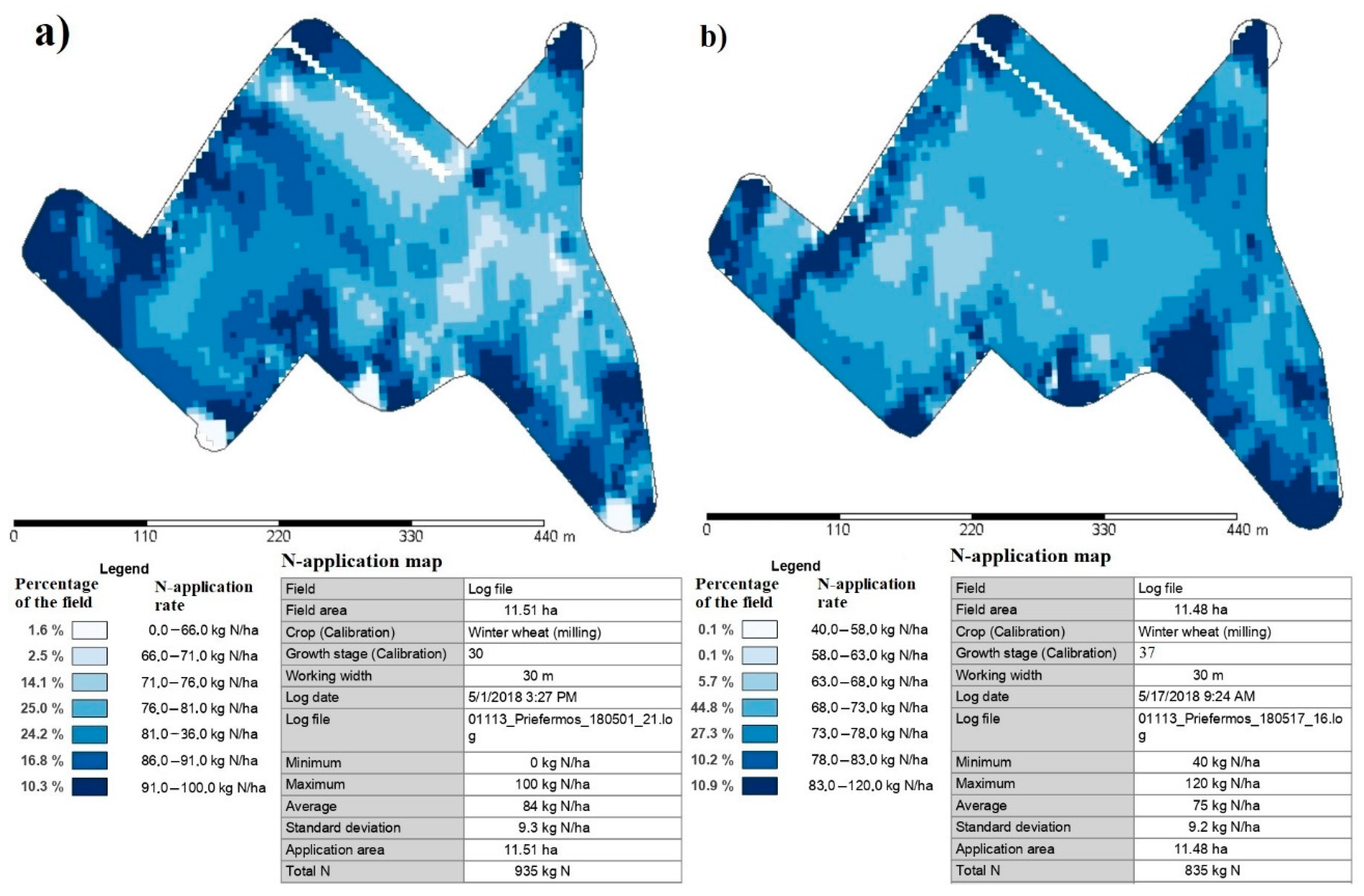
3.2. Additional N-Variable Rate Fertilization of Winter Wheat

This study presents additional fertilization of winter wheat at growth stages BBCH 30 and BBCH 37. In spring 2018, N uptake (Figure 8) and N fertilization maps (Figure 9) were generated with additional N fertilization at a variable rate in real-time with the Yara N-Sensor ALS. N uptake was highest in 15.2% of the total area (56–67 kg ha⁻¹), and N application rate was lowest in 16.6% of the total area (66–76 kg ha⁻¹) (Figure 8a). In the areas where crop N uptake was below the biomass threshold (17 kg ha⁻¹ at BBCH 30), the fertilization rate was reduced from 66 to 0 kg ha⁻¹ (1.6% of the total area).

During variable fertilization at BBCH 37 (Figure 8b), the average N uptake of winter wheat was 108 kg ha⁻¹ and the average N fertilizer rate was 75 kg ha⁻¹. In the last additional fertilization, the field became more homogeneous. For example, when the N uptake went from 105 to 117 kg ha⁻¹, the field uniformity reached 84.3%. The uniformity of the field (71% of the total area) also affected the fertilizer application rate, which ranged from 68 to 78 kg ha⁻¹. After 16 days, N fertilization change in N uptake at BBCH 37 was on average 60 kg ha⁻¹.

3.3. Crop Yield

For calculation of the demand of mineral fertilizer, energy, and pollution indicators, the average yields were determined using historical yield data in this field from the last 4 years for each crop in the crop rotation. The average yields for spring barley, winter oilseed rape, winter wheat, and faba beans were 7.0, 5.0, 8.0, and 4.0 t ha⁻¹, respectively. These yields were taken as assumed and used in subsequent calculations as yields obtained using the FRF method. The average yields for the whole field using the VRF method for spring barley, winter oilseed rape, winter wheat, and faba beans were 7.3, 5.2, 8.1, and 3.9 t ha⁻¹, respectively.

During the threshing of winter wheat, a precise yield map was created (Figure 10) and yield data were recorded: An average of 8.1 t ha⁻¹, a minimum of 5.4 t ha⁻¹, a maximum of 9.2 t ha⁻¹. After comparing the yield map with the N uptake map, it can be seen that the highest yield was in the places with the lowest N application rate, because in this site, specific areas contained more available N nutrients than other areas. During the application of variable N fertilization in the places where the maximum rate of 220 kg ha⁻¹ was applied, the lowest yield was 5.4 t ha⁻¹. The reason could be that these site-specific areas had lower N availability in the soil. The N uptake map made at growth stage BBCH 37 showed more even nitrogen distribution in the crop matching to the yield map with smaller yield variability in the field. In 64% of the total area, the yield uniformity ranged from 6.8 to 8.4 t ha⁻¹.

The threshing speed of the combine was uniform and accounted for 68% of the total threshing area in the range from 3.5 to 4.1 km h⁻¹. The average threshing rate of winter wheat was 3.7 km h⁻¹ with average grain moisture of 14.4% and a yield of 8.1 t ha⁻¹. Feiffer et al. [33] found that a more even crop of winter wheat resulted in a higher threshing rate of 9–33%.

Grain moisture was also uniform and accounted for 75% of the total area in the range of 13.8–14.9% moisture. More evenly dried grain can be threshed earlier, and more even threshing speed results in higher harvester’s performance.

The highest yield of winter wheat 9.2 t ha⁻¹ was obtained by performing two additional fertilizations at growth stages BBCH 30 and BBCH 37 in the places where the lowest amount of N fertilizer was applied at a variable rate of 139 kg ha⁻¹.

3.4. Fertilizer Use and Savings

The results of comparison of VRF based on field soil analysis and crop nutrient demand with FRF, which takes into account only crop nutrient removal with the assumed average yield (

Table 3. Fertilization rates and fertilizer reduction indicators.

Year	Crop	Predicted Yield (t ha−1)	Fertilizer	Removal of Fertilizer with Yield (kg ha−1)	Fertilization Rate (kg ha−1)
					VRF	FRF	Difference between FRF and VRF	Reduction per 1.0 t of Yield
2016	Spring barley	7.0	N	122.5	50.0	50.0	0.0	0.0
			P2O5	56.0	33.0	56.0	23.0	3.3
			K2O	42.0	25.7	42.0	16.3	2.3
2017	Winter oilseed rape	5.0	N	250.0	175.0	188.0	13.0	2.6
			P2O5	89.3	33.0	89.3	56.3	11.3
			K2O	49.8	25.7	49.8	24.1	4.8
2018	Winter wheat	8.0	N	184.0	199.0	210.0	11.0	1.4
			P2O5	64.0	33.0	64.0	31.0	3.9
			K2O	48.0	25.7	48.0	22.3	2.8
2019	Faba Bean	4.0	N	240.0	70.2	70.2	0.0	0.0
			P2O5	47.6	33.0	47.6	14.6	3.6
			K2O	56.0	25.7	56.0	30.3	7.6
Total all years			N	819.5	494.2	518.2	24.0	-
			P2O5	256.9	132.1	256.9	124.8	-
			K2O	195.8	102.7	195.8	93.1	-
Total field					729.0	970.9	241.9

Notes: VRF–variable rate fertilization; FRF–fixed-rate fertilization.

). The results showed that less fertilizers were consumed when using the VRF method in 4-years compared to FRF: N 24 kg ha⁻¹ (4.6%), P₂O₅ 124 kg ha⁻¹ (48.6%), K₂O 93.1 kg ha⁻¹ (47.5%), respectively. The amounts of P element in the soil before the start of the experimental studies were higher (on an average three times in the whole field) than the recommended optimal amount. Therefore, in the phosphorus fertilization maps for variable fertilization, the rate of phosphorus fertilizers was reduced. A fixed rate of phosphorus fertilization was determined at the traditional recommended rate for each crop as shown in Table 3. These reasons resulted in more phosphorus savings than other fertilizers (N and K₂O). Other researches stated that applying VRF of phosphorus fertilizer during the study period decreased the variability of the amount of this element in the soil [26]. The second-highest savings were achieved using potassium fertilizers, and average K₂O level stayed at the optimum level at the end of the study. However, it needs to be clarified that the smallest N savings were achieved because variable N application software was created not for all crops. In our study, N application software was used only for winter wheat and oilseed rape. This could be the main reason why so little savings was found in N-fertilizer during the 4-year crop rotation. Other research have recorded 4 to 37% of nitrogen fertilizer savings in wheat in Turkey [4]. Yara International Research Centre (Hanninghof, Germany) applied tested winter wheat fertilization with N fertilizer at a variable rate with Yara N-Sensor in 2001–2005. Their test resulted in 12% lower fertilizer consumption compared to uniform fertilization [34]. Koch et al. [35] found that variable rates of maize fertilization can save from 6 to 46% of the fertilizer compared to a uniform rate. Other researchers compared urea fertilization between FRF (105 kg ha⁻¹) and VRF (64 kg ha⁻¹) in maize production. According to Greenseeker’s recommendation, they obtained an average yield of 3.9 t ha⁻¹ in both fertilization methods [36].

Our research found that the total amount of saved NPK fertilizers was 241.6 kg ha⁻¹. In 4-years, from the total field were saved: 1418.8 kg of P₂O₅, 1058.3 kg of K₂O, 272.9 kg of N. Depending on the crop type, NPK fertilizer savings were uneven. The highest NPK fertilizer savings were in winter oilseed rape–1061.8 kg (28.6%), spring barley–446.7 kg (40.1%), winter wheat–731.0 kg (20.0%), and faba beans–510.4 kg (43.3%). The research showed that while maintaining the optimal average nutrient content in the field, less fertilizer was used to grow different crops.

3.5. Energy Use Reduction with VRF

Compared VRF with FRF in spring barley (2016), energy consumption related to P₂O₅ and K₂O fertilizers was lower at 41.0% and 38.9%, respectively (

Table 4. Comparative energy consumption and reduction indicators using VRF and FRF.

Year	Crop	Predicted Yield (t ha−1)	Fertilizer	Energy Equivalent (MJ kg−1)	Energy Input (MJ ha−1)				Energy Reduction MJ per Total Field Area (MJ Field−1)
					VRF	FRF	Difference between FRF and VRF	Reduction per 1.0 t of Yield
2016	Spring barley	7.0	N	60.6	3030	3030	0.0	0.0	0.0
			P2O5	11.1	366.6	621.6	255.0	36.4	2899
			K2O	6.7	172.1	281.4	109.3	15.6	1243
2017	Winter oilseed rape	5.0	N	60.6	10605	11393	787.8	157.6	8957
			P2O5	11.1	366.6	991.2	624.6	124.9	7102
			K2O	6.7	172.1	333.7	161.6	32.3	1837
2018	Winter wheat	8.0	N	60.6	12059	12726	666.6	83.3	7579
			P2O5	11.1	366.6	710.4	343.8	43.0	3909
			K2O	6.7	172.1	321.6	149.5	18.7	1700
2019	Faba bean	4.0	N	60.6	4254	4254	0.0	0.0	0.0
			P2O5	11.1	366.6	528.4	161.7	40.4	1839
			K2O	6.7	172.1	375.2	203.1	50.8	2310
Total all years			N	60.6	29,949	31,403	1454	-	16,537
			P2O5	11.1	1467	2852	1385	-	15,748
			K2O	6.7	688.2	1312	623.6	-	7091
Total field					32,103	35,566	3463	-	39,375

Notes: VRF–variable rate fertilization; FRF–fixed-rate fertilization; total field area–11.37 ha.

). N variable fertilization was not applied for spring barley.

In 2017 for winter oilseed rape applying VRF, energy consumption related to fertilizer P₂O₅ was lower 63.0%, K₂O–48.4% and N–6.9%, compared to FRF.

In 2018 for winter wheat using VRF, energy consumption related to P₂O₅ fertilizers was lower 48.4%, K₂O–46.5% and N–5.2%, compared to FRF practice.

In 2019 for faba beans applying VRF, energy consumption related to P₂O₅ fertilizers was lower 30.6%, K₂O–54.1%, compared to FRF method. N variable fertilization was not applied for faba beans.

Comparing VRF with FRF, the lowest energy savings were obtained by fertilizing winter wheat with N fertilizers, the highest–faba beans with K₂O.

Summarizing the crop rotation in 4-years, when the VRF fertilization method was applied, energy consumption for phosphorus fertilizers was 48.6% lower and for potassium fertilizers–47.5% lower compared to the FRF fertilization method. Energy consumption related to nitrogen fertilizers was 4.6% lower compared to FRF. With variable fertilization, the total energy consumption for all fertilizers was 9.7% lower compared to FRF. The results showed that energy savings by reducing the application of P and K were generally lower compared to N fertilizer with respect to the energy use per ha due to fertilizer application. Summarizing the study’s data on the energy consumption associated with NPK fertilizers over 4-years in the entire experimental field, it was found that the energy consumption of VRF was reduced by 9.7% Field⁻¹ compared to the FRF method.

3.6. Changes in Fertilization Reduce Environmental Pollution

By applying VRF according to a pre-arranged fertilization plan and using fertilizer application maps and efficient distribution equipment, we can reduce both fertilizer costs as well as GHG emissions. Comparison of a 4-year VRF with FRF method allowed concluding that lower GHG emissions were obtained due to the use of fertilizers: 119.0 kg CO_2eq ha⁻¹ of N, 168.5 kg CO_2eq ha⁻¹ –P₂O₅, 54.0 kg CO_2eq ha⁻¹–K₂O, respectively (

Table 5. Reduction of GHG emissions by using variable and fixed rates of fertilization.

Year	Crop	Predicted Yield (t ha−1)	Fertilizer	GHG Equivalent (kg CO2eq kg−1)	GHG Emission (kg CO2eq ha−1)				Reduction GHG Emission for Total Field Area (kg CO2eq Field−1)
					VRF	FRF	Difference between FRF and VRF	Reduction per 1.0 t of Yield
2016	Spring barley	7.0	N	4.96	248.0	248.0	0.0	0.0	0.0
			P2O5	1.35	44.6	75.6	31.0	4.4	352.6
			K2O	0.58	14.9	24.4	9.5	1.4	107.6
2017	Winter oilseed rape	5.0	N	4.96	868.0	932.5	64.5	12.9	733.1
			P2O5	1.35	44.6	120.6	76.0	15.2	863.7
			K2O	0.58	14.9	28.9	14.0	2.8	159.1
2018	Winter wheat	8.0	N	4.96	987.0	1042	54.6	6.8	620.4
			P2O5	1.35	44.6	86.4	41.8	5.2	475.4
			K2O	0.58	14.9	27.8	13.0	1.6	147.2
2019	Faba beans	4.0	N	4.96	348.2	348.2	0.0	0.0	0.0
			P2O5	1.35	44.6	64.3	19.7	4.9	223.6
			K2O	0.58	14.9	32.5	17.6	4.4	200.0
Total all years			N	4.96	2451	2570	119.0	-	1354
			P2O5	1.35	178.4	346.8	168.5	-	1915
			K2O	0.58	59.6	113.6	54.0	-	613.8
Total field					2689	3031	341.5	-	3883

Notes: VRF–variable rate fertilization; FRF–fixed-rate fertilization; total field area–11.37 ha.

). Similar research in Latvia showed that a variable N fertilizer application in winter wheat reduced GHG emissions by 46.8 kg CO_2eq ha⁻¹ or 6% compared to a fixed rate N fertilizer application technology [37].

Our study found an overall reduction in GHG emissions of 341.5 kg CO_2eq ha⁻¹. Most greenhouse gas emissions reductions using the VRF method were achieved with P₂O₅ (168.5 kg CO_2eq ha⁻¹). Fertilization with NPK fertilizers in the whole field at a variable rate over 4-years reduced the GHG emissions by 3882.6 kg CO_2eq (11.27%). This study shows that GHG emissions in the experimental field decreased over 4-years, depending on the type of fertilizer: 48.6% for P₂O₅, 47.5%–K₂O and 4.6%–N, respectively. Balafoutis et al. [16] reported that the use of VRF technology can reduce the GHG emission potential of 5% attributed to the use of N mineral fertilizers without yield effects. Italy scientist’s findings suggest that VRF is able to decrease CO₂ emission in comparison with FRF [38].

According to the crop rotation, different GHG emissions were obtained by growing different crops and applying VRF, compared to FRF method in the whole study field: 460.2 kg CO_2eq Field⁻¹ for spring barley, 1755.9 kg CO_2eq Field⁻¹–winter rape, 1242.9 kg CO_2eq Field⁻¹–winter wheat, 423.6 kg CO_2eq Field⁻¹–faba beans, respectively. The study showed that the greatest savings in GHG emissions were achieved in winter oilseed rape.

3.7. Economic Benefits

An evaluation of the economic benefits of changing a fixed fertilization rate to a variable rate in order to save the cost for fertilizers for the entire research field over 4 years was performed. It was revealed that when the price of N was 0.9€ kg⁻¹ and the amount of fertilizer used was 272.9 kg, the economic benefit was achieved 21.6€ ha⁻¹. When the price of the fertilizer P₂O₅ was 0.8€ kg⁻¹ and K₂O 0.5€ kg⁻¹ and their consumption was 1418.8 and 1058.3 kg, then the savings were 99.8 and 46.5€ ha⁻¹, respectively. The total 4-year economic benefit for the whole field due to the savings on NPK fertilizers was 168.0€ ha⁻¹. Other researchers [34], who compared fertilization at a fixed rate with the one at a variable rate, calculated an economic benefit of 19$ (~16.4€) per hectare from savings on nitrogen fertilizers. Diacono et al. [3] analyzed the cost-effectiveness of variable rate N fertilizer management methods in wheat crops and concluded that real-time N-based management had the higher profitability, ranging from 5 to 60$ ha⁻¹ (~4.3 to ~51€ ha⁻¹) compared to FRF. Dobermann et al. [39] found that fertilization of rice with NPK fertilizers using VRF can increase the yields by 12% compared to FRF.

A comparative analysis of the yields showed that VRF had an advantage over FRF due to higher crop yields. In our studies, no actual yield results were obtained using fixed rate fertilization. Yields for all four plants were assumed on the basis of average values from previous years. Using the VRF system, the yields of different crops obtained were very similar to the assumed yields used for the FRF method. Other authors also found that the average wheat grain yield was 4.24 t ha⁻¹ and the mean increase in wheat grain yield applying VRF was 0.8% when compared with the FRF treatment averaged over 10 sites and two years [40]. In the study of scientists from Italy, there were no significant differences of the barley grain yield between FRF and VRF technologies observed [38]. The method used to apply variable N fertilization has been proved to be effective, leading to a similar barley yield to conventional practice while using less fertilizer (75 kg N ha⁻¹). The VRF method has been proved to be a valid alternative to conventional fertilization, considering economic evaluation and leading a saving of 266€ ha⁻¹ [38].

All crops yielded economic benefits, except for faba beans. A 4-year benefit due to the increased yield was 108.0€ ha⁻¹. Comparing VRF and FRF methods of spring barley, winter oilseed rape, winter wheat and faba beans, the economic benefits from the yield were 45, 70, 17 and −24€ ha⁻¹, respectively. Economic benefit from yield was calculated using the grain price for each crop: 150€ ha⁻¹ for spring barley, 350€ ha⁻¹–winter oilseed rape, 170€ ha⁻¹–winter wheat and 240€ ha⁻¹–faba beans, respectively.

The greatest savings of energy input and GHG emissions were obtained with N and P₂O₅ fertilizers at a variable rate in winter oilseed rape. Comparing different fertilizers, the best cost savings results were achieved using P₂O₅ fertilizers for winter oilseed rape, winter wheat, and spring barley 45, 24.8, and 18.4, respectively. For all fertilizers, energy inputs, GHG emissions, and cost savings using VRF comparing to FRF are presented in Figure 11.

Summarizing the research results obtained in this study, it can be stated that variable fertilization is an important technological process that reduces the consumption and the costs of NPK fertilizers, saves energy costs, and contributes to the preservation of a cleaner environment. In order to achieve even stronger positive energy, as well as economic and environmental impact, future research needs to investigate the technological processes of not only fertilization but also of sowing and spraying of plant protection products at a variable rate.

4. Conclusions

A 4-year study of soil elements showed that even after 4-years of using VRF, excess phosphorus of 48.5 mg per 100 g of soil and potassium with 27.6 mg per 100 g of soil were still present in certain field areas. Repeated soil element analysis showed that application of VRF, taking into account the existing nutrient content in the soil and demand of elements for the crop, can save fertilizers and reduce environmental impact without over-fertilizing P₂O₅ and N in the areas where there was already an excess of these elements. In the experimental field, the application of VRF maps allowed avoiding over-fertilization in separate field locations, thus saving fertilizers and making the obtained yield closer to the planned one. Application of this method allowed reducing the costs of fertilizers: 4.6% for N, 48.6%—P₂O₅ and 47.5%—K₂O. The total consumption of NPK fertilizers was lower by 24.9% compared to the FRF. Thus, variable rate fertilization results in higher fertilizer use efficiency.

Lower consumption of mineral fertilizers resulted in lower energy consumption throughout the 4-year crop rotation. With VRF, the total energy input for all fertilizers was 3463.1 MJ ha⁻¹ or 9.74% lower than with FRF. The largest reduction in energy consumption was found for nitrogen and phosphorus fertilizers, 1454.4 and 1385.1 MJ ha⁻¹, respectively. Lower spreads of fertilizers all over the field resulted in lower GHG emissions to the environment during the study period. Phosphorus and potassium VRF application was estimated to reduce the GHG emissions by almost twice compared to FRF. For the total amount of NPK fertilizers, 11.3% lower GHG emissions were obtained. At the end of the study, GHG emission reductions of 341.5 kg CO_2eq ha⁻¹ or 3882.6 kg CO_2eq Field⁻¹ were determined.

VRF, according to the application plan and by using VRF maps, allowed a reduction in NPK fertilizers by 241.9 kg ha⁻¹ or 2750.0 kg Field⁻¹. A significant decrease in the need of mineral fertilizers reduced production costs and contributed to cleaner agricultural production. The total economic benefit coming from the saved funds for fertilizers due to an application of VRF was 168.0€ ha⁻¹ or 1909.7€ Field⁻¹.

Based on the results of our study, we can say that the application of the VRF method allows farmers to benefit from lower costs for fertilizers and, at the same time, helps them to meet the EU’s requirements for environmental pollution in agriculture. The energy, economic, and environmental benefits of variable rate fertilization are a great recommendation to continue this type of research in the future, including more details on precision farming such as variable rate sowing, spraying of growth regulators, and plant protection products.