Article

Banana Biomass Estimation and Yield Forecasting from Non-Destructive Measurements for Two Contrasting Cultivars and Water Regimes

1
Department of Biosystems, KU Leuven, Willem De Croylaan 42—Box 2455, 3001 Heverlee, Belgium
2
Division of Soil and Water Management, KU Leuven, Celestijnenlaan 200e—Box 2411, 3001 Leuven, Belgium
3
International Institute of Tropical Agriculture, IITA, Arusha P.O. Box 447, Tanzania
4
Nelson Mandela African Institution of Science and Technology, NMAIST, Arusha P.O. Box 447, Tanzania
5
Bioversity International, Willem De Croylaan 42, 3001 Heverlee, Belgium
*
Author to whom correspondence should be addressed.
Agronomy 2020, 10(9), 1435; https://doi.org/10.3390/agronomy10091435
Submission received: 13 July 2020 / Revised: 16 September 2020 / Accepted: 18 September 2020 / Published: 21 September 2020

Abstract

:
The largest abiotic constraint threatening banana (Musa spp.) production is water stress, impacting biomass buildup and yields; however, so far no studies have investigated the effects of water stress on allometric equations in banana. Weighted least square regression models were built for (i) estimating aboveground vegetative dry biomass (ABGVD) and corm dry biomass (cormD) and (ii) forecasting bunch fresh weight (bunchF), based on non-destructive parameters for two cultivars, Mchare Huti-Green Bell (HG, AA) and Cavendish Grande Naine (GN, AAA), under two irrigation regimes: full irrigation (FI) and rainfed (RF). FI affected growth, yield, and phenological parameters in the field (p < 0.05) depending on the onset of moisture stress. Pseudostem volume (Vpseudo) proved a good predictor for estimating ABGVD (R2adj = 0.88–0.92; RRMSE = 0.14–0.19), but suboptimal for cormD (R2adj = 0.90–0.89, RRMSE = 0.21–0.26 for HG; R2adj = 0.34–0.57, RRMSE = 0.38–0.43 for GN). Differences between RF and FI models (p < 0.05) were small as 95%CI overlapped. Vpseudo at flowering predicted bunchF in FI plots correctly (R2adj = 0.70 for HG, R2adj = 0.43 for GN; RRMSE = 0.12–0.15 for HG and GN). Differences between FI and RF models were pronounced as 95%CI did not overlap (p < 0.05). Bunch allometry was affected by irrigation, proving bunchF forecasting needs to include information on moisture stress during bunch filling or information on bunch parameters. Our allometric relationships can be used for rapid and non-destructive aboveground vegetative biomass (ABGVD) assessment over time and to forecast bunch potentials based on Vpseudo at flowering.

1. Introduction

Banana (Musa spp.), the most important fruit worldwide [1], is a long cycle crop with a vegetative phase between 7–13 months depending on environmental conditions, such as water and nutrients [2]. For most of the plant’s life, it develops without a bunch. Bunch biomass is linked to biomass buildup during the vegetative phase (aboveground: pseudostem, petioles and leaves, and belowground: corm) [3], as assimilates are translocated from within the banana mat to the bunch after bunch emergence [2,4,5]. Monitoring vegetative biomass enables the following of growth over time and, due to its link with yields, can provide an indicator of future yields.
Monitoring biomass over time can be done by destructive whole-plant sampling, but it is more practical to quantify the biomass during the growth cycle or to forecast the yield from non-destructive observations using allometric relationships. Destructive sampling is very labor intensive, time consuming, and provides only one sampling point for one plant. To capture biomass over time, plants need to be sampled periodically, requiring lots of plants and space. Sampling plants before they are harvest ready also stands in the way of quantifying bunch weights.
Allometric relationships specify how growth and size in plants or plant components is related to their allocated biomass [6,7]. Parameters can be vegetative characteristics (e.g., pseudostem girth at base) [3,5,8,9,10,11], bunch components (e.g., number of hands, fingers, finger volume) [12,13] or phenological observations (e.g., days to flowering, days to harvest). Vegetative parameters that are well connected to biomass, and/or parameters that are connected to future yields and allow bunch weight ‘forecasting’, are of significant interest. Measuring such parameters in the field is much faster than destructive sampling, and leaves fields intact. Allometric equations are useful for periodic biomass monitoring in the field [9] which is needed to calibrate and further improve computer crop simulation models [5,14,15]. Crop models can be used (among others) to analyze management interventions under different environments, to mitigate and adapt crop production to climate change [12,16,17] and for economic analysis to manage financial decisions (e.g., manpower and cost of agricultural inputs as irrigation) [15]. As allometric relationships are the foundation of such models, correct relationships are of crucial importance.
Allometric relationships were previously developed for a limited number of banana cultivars for both vegetative and bunch biomass estimation. Nyombi et al. [5] developed allometric relationships for both biomass and bunch weight estimation for two East African highland banana (EAHB) cultivars (Mbwazirume and Kisansa) with data from two locations under various nutrient regimes. Their models followed a power function using girth and height of pseudostem as predictors, whereby covariates included banana phenological stages (vegetative, flowering, and harvest). Plants were irrigated, but with unspecified amounts of water, and fresh bunch weights ranged from 20–40 kg plant−1, indicating stressed conditions. Pooling data across cultivars and growth stages lead to a high R2 (>0.7) but increased the variance in biomass estimations. Model performance increased when data were partitioned between growth stages, indicating that allometric relationships vary with the growth stage. Yamaguchi and Araki [10] estimated biomass components using linear regression models based on pseudostem volume (Vpseudo) for EAHB cultivars from farmers’ fields. Models had good fits (R2 = 0.93) but the plant sample was small (n = 14) and stress could not be excluded as plants were rainfed. Negash et al. [8] estimated biomass based on pseudostem diameter and height in Enset (Ensete ventricosum), another genus of the Musaceae. Models performed well for total biomass estimation (R2 > 0.89), but plants came from rainfed farmers’ fields without information on potential stresses.
Allometric models for bunch weight estimation were previously created, but these include parameters that change until harvest so cannot be used in forecasting bunch weights. Soares et al. [12] estimated bunch weights using multiple linear regression and neural networks for an AAAB tetraploid hybrid. Models were accurate (R2 > 0.71), but predictors included variables that can only be measured in a destructive manner at harvest (e.g., average fruit weight at harvest). Woomer et al. [13] estimated bunch weights for a rainfed EAHB cv. Mbwazirume based on estimated bunch volume through linear regression (R2 = 0.85–0.94), but as bunch volume changes until harvest [2], yields were not forecasted and no information on potential stress was given. Wairegi et al. [9] quantified bunch weights of 39 triploid EAHB cultivars from 179 farms in Uganda, whereby multiple linear regression models used pseudostem girth at base and height at 1 m, number of hands, and number of fingers in the lower row of the second hand as predictors. Data partitioning along cultivars, developmental stages, and regions improved model accuracy but differences were not significantly different compared to the pooled dataset. Plants were rainfed and given the wide range of bunch weights in this study (2–60 kg plant−1) stress from multiple sources was presumed, but its effect on allometry was not analyzed.
The major constraint in all previously developed allometric models is that fields were not growing under optimal conditions as they were stressed by inadequate amounts of water and/or nutrients. Water (excess and deficit) is the most limiting abiotic constraint to banana production [18]. Suboptimal rainfall may lead to significant reduction in vegetative parameters (e.g., pseudostem height, girth), bunch components (number of hands, number of fingers, individual finger weight, fruit filling) [19], and may delay phenological events as flowering or harvest [20,21]. Parameters underlying allometric models are often impacted by moisture, but the overall effect on the relationship between a parameter and allocated biomass due to soil moisture is not specified in earlier allometric models. Their general use and applicability can be questioned. Similar genotypes may lead to different biomass allocation patterns and phenotypes under different biotic and abiotic environments [22], and banana has shown dry matter allocation plasticity due to drought and soil nutrients [23] and plant density [24]. Furthermore, due to the large phenotypic and or genetic differences between banana cultivars, allometric models can differ between cultivars [5,9].
So far, no research has compared allometric models between differently irrigated plants in the same field. As allometric models relate growth and size, which are affected by soil moisture, to accumulated biomass, we are interested to check whether allometric relationships remain similar under different soil moisture regimes.
The objective of this research was three-fold:
Firstly, to assess the effect of soil moisture on growth parameters, phenology and growth rates using two distinctly different cultivars: the EAHB cv. Mchare—Huti Green Bell (AA), a diploid, and the Cavendish—Grande Naine (AAA), a triploid of immense commercial appeal.
Secondly, to use easily observable plant growth parameters to establish allometric relationships in both cultivars for (i) vegetative biomass estimation (aboveground: pseudostem, petioles, and leaves and belowground: corm) to allow monitoring vegetative biomass production over time, and (ii) bunch weight forecasting to allow quantifying bunch weights before harvest.
Thirdly, to compare these allometric relationships across water regimes for both cultivars to assess whether banana plasticity under drought results in significant different relationships. As drought readily affects vegetative parameters, yield, and phenology [2,18,22], we hypothesize drought to significantly influence allometric relationships of both vegetative biomass estimation and bunch weight forecasting.

2. Materials and Methods

2.1. Experimental Design

Experiments were established in fields of the International Institute of Tropical Agriculture (IITA) and the Nelson Mandela African Institution of Science and Technology (NM-AIST) in Arusha, Tanzania (3°23′58″ S, 36°47′48″ E) at an altitude of 1188 m asl as described in detail in Stevens et al. [25]. Soils are Endocalcic Phaeozems (Geoabruptic, Clayic, Humic) [26], moderately shallow to deep (90–120 cm) with a silty clay loam to silty clay texture. The climate is a tropical highland climate with a moderately cool thermal zone. Rainfall follows a bimodal yearly pattern with a long rainy season extending from late March to early June and a shorter rainy season from October to December, although rainfall is variable from year to year [25,27].
Total precipitation received during the experiment was about 903 mm year−1 for HG, and 913 mm year−1 for GN, lower than those for optimal banana production (1100–2650 mm year−1) and not evenly spread (dry spells of more than two months) (Figure 1a) implying the need for irrigation [19,28,29].
Two experiments were carried out differing in cultivar and date of planting over the course of two full crop cycles (until harvest of C2). Planting material was provided by IITA, Arusha, Tanzania and Crop Bioscience Solutions Ltd, Arusha, Tanzania. In experiment 1, the EAHB Huti Green Bell (HG, Musa AA Mchare subgroup) was planted on 3 May 2017. In experiment 2, Grande Naine (GN, Musa AAA Cavendish subgroup) was planted on 17 November 2017. The diploid HG is characterized by a slender tall pseudostem, with erect foliage and a bunch that bears fruits with marked ridges [30]. The triploid GN is characterized by a short, thick pseudostem, with semi-drooping foliage and producing almost round fingers [31]. Both cultivars are of significantly different phenotypical constitution. Planting material for both experiments consisted of in vitro plants, hardened in growth chambers and screen houses. Plant spacing was 2 m (row) × 3 m (line) leading to 1666 plants ha−1.
The design was a blocked design with drip irrigation as treatment but given the infrastructure the irrigation treatments could not be randomized (Figure S1). In experiment 1, two blocks were planted with HG. Each block contained five rows of 15 mats, subdivided in three plots of 25 mats (5 × 5), of which the central nine mats (3 × 3) were used for continuous data collection. Each block consisted of a different irrigation treatment. For HG, there were three plots for each treatment. Border mats were used for periodic destructive sampling. In experiment 2, four blocks were planted with GN. Each block contained five rows of 14 mats, subdivided in two plots of 35 mats (7 × 5), receiving two different irrigation treatments. The central nine mats (3 × 3) in each plot were used for continuous growth data collection, leading to four replications (plots) per treatment. The first and last two mats of each row (2 × 5 mats) together with the border rows were used for periodic destructive sampling. Each treatment was replicated four times across the blocks.
All mats received irrigation for the first four months post-transplant (establishment period, four MAP). Thereafter, two irrigation treatments were applied: optimal ‘full’ irrigation (FI) and rainfed (RF), based on volumetric water contents in the root zone (as determined by Time Domain Reflectometry) (Figure 1b). In the FI treatment, mats received water whenever more than 25% of total available water in the root zone was depleted. No supplemental irrigation was provided in RF treatments after the initial four month establishment period, leading to divergence of soil moisture between RF and FI in HG and GN closely following the dry seasons (Figure 1a,b). In HG, soil moisture first became significantly different at 23 weeks after planting (WAP) (October 2017) until 45 WAP (March 2018) during the vegetative stage of C1, followed by a rainy season after which they diverged again from 55 WAP (May 2018). In GN, RF plots became significantly more depleted from 27 WAP onwards (May 2018), close to the onset of flower emergence of C1 [25], therefore in GN most of the vegetative growth of C1 occurred under similar soil moisture in RF and FI plots.
Irrigation and precipitation combined, FI plots received approx. 3100 mm (HG) and 4003 mm (GN) over the entire growing season (until harvest of C2), compared to RF plots which received 1916 mm (HG) and 2549 mm (GN). FI plots received approx. 1522 mm year−1 (HG) and 2000 mm year−1 (GN). RF plots received approx. 935 mm year−1 (HG) and 1297 mm year−1 (GN). For a more detailed explanation on the onset of moisture stress and its effect on leaf formation and canopy cover in these fields, the reader is referred to Stevens et al. [25].
Mats received an optimal mixture of mineral fertilizers and manure, to exclude nutrient stresses [32]. Mineral fertilizers were split applied: 153 kg N ha−1 year−1 (urea), 206 kg K ha−1 year−1 (Muriate of potash), 19.26 kg Mg ha−1 year−1, and 25.6 kg S ha−1 year−1 (MgSO4) were applied monthly in the rainy season and every two months in the dry season, while 40.2 kg P ha−1 year−1 (triple super phosphate) was applied every five months. Twenty L of fresh farmyard cow manure was applied per mat twice yearly before the start of the rainy season.
All suckers were allowed to grow until four MAP after which suckers were selected for C2 (Figure S2). Afterwards, suckers were pruned on a monthly basis until bunch filling of C1, when a sucker for C3 was chosen. Maximally, three generations were allowed to grow at any time. Weeds and dead leaves were cut monthly and removed from the field. No pests were present in the field. No disease control was applied, except for Black Sigatoka (Pseudocercospora fijiensis) in the wet season, when moderately infected leaves were pruned to avoid further spread of this fungus [25].

2.2. Plant Data Collection

Growth data included periodic non-destructive growth data and destructive data (Table 1).
Non-destructive growth data were measured monthly at the plot level (3 × 3 mats), on all individual plant cycles (cycle 1, C1; cycle 2, C2 and cycle 3, C3) present on the mat until harvest of C2 (Table 1). The main plant is the oldest plant on a mat, whereby ratoon plants (sucker) are new selected shoots springing from the base of the plant. To address multicollinearity, measured parameters were recombined into new parameters as pseudostem volume (Vpseudo), leaf area index (LAI), Vfinger, and Ratiofinger (Table 1).
Leaf areas were estimated by measuring leaf length, leaf width, and using an experimentally determined leaf area factor (laf) as explained by Stevens et al. [30]. LAI was determined by summing the area of all the leaves on a banana plant and dividing it by the ground area for each mat.
Phenological events as days to flowering (DTF) and days to harvest (DTH) were noted for each plant on a mat. As C3 has not fully flowered and harvested, phenological events were only presented for C1 and C2 (Table 2). For C1, the DTF and DTH were determined from planting. For C2, the DTF and DTH were determined from the moment of sucker selection until flowering and harvest. Flower cycle duration (FCD) notes the duration in days between flower emergence of C1 and C2 (successive cycles) on the same mat, and harvest cycle duration (HCD) notes the duration in days between successive harvest of C1 and C2 on the same mat.
The pseudostem volume at flower emergence (Vpseudo, Flower) and the LAI at flower emergence (LAIFlower) were interpolated for flowering dates through local non-parametric regression (loess) on the Vpseudo and LAI data collected over the growing season (Figure S3). Similarly, the Vpseudo and LAI of the follower (S for sucker) of the flowering main plant was determined (Vpseudo, FlowerS and LAIFlower,S).
Biomass component weights (pseudostem, leaf, petiole, bunch, and corm) were measured destructively during ‘harvest’ and ‘periodic destructive sampling’.
At ‘harvest’, harvest-ready plants of C1 and C2 showing ripe bunches were cut down at the base of the pseudostem, but succeeding cycles were left on the mat. Non-destructive vegetative and bunch characteristics (Table 1) were determined on the harvested plant together with destructive biomass. Fresh weight of vegetative components (pseudostem, leaf, petioles) and bunch (bunchF) was measured using a field balance (±0.05 kg), and subsamples were taken, chopped and dried at 80 °C for 48 h in a hot-air oven (to not destroy plant tissue) until subsample weights did not vary anymore to determine the dry matter percentage (Table S1). Aboveground vegetative dry matter (ABGVD) included the pseudostem, petioles, and leaves. Hereafter, when using the term ‘harvest’, plants that are harvest ready for their bunches were noted.
At ‘periodic destructive sampling’, entire mats were randomly sampled every three months from planting onwards to obtain a database of plants spanning different sizes and growth stages including C1, C2, and C3 plants. From planting onwards, every three months, mats (n = 3) were randomly chosen from border rows or from destructive sampling areas in each treatment in both experiments. Whole mats were excavated and for each individual cycle, growth data were measured (Table 1) and biomass components (corm, pseudostem, petioles, leaves, bunch) were separated and weighted. Non-differentiated suckers (not protruding above ground level) were counted as part of the corm. All cycles present on a mat (C1, C2, and C3) were used for data collection. ABGVD was calculated similarly as at harvest. Corms were separated per cycle, weighted and corm dry matter (cormD) was calculated based on fresh corm weight and subsample dry matter percentages (Table S1).

2.3. Moisture Effect on Plant Growth

Kruskall–Wallis non-parametric tests (α = 0.05) for multiple comparison of growth parameters between irrigation treatments, cultivar, and growth cycle were applied on collected growth data at flowering and harvest of C1 and C2 (Table 2).
As the effect of added water (precipitation and irrigation) is very dependent on the environment in which a plant develops the ratio (R) of cumulative water added (W) and cumulative ET0 was determined for each plant between: planting and flowering (RPF), flowering and harvest (RFH), and planting and harvest (RPH) (Table 2).
The average pseudostem growth rate (Vrate, Table 1), an indicator of vegetative growth was analyzed in terms of RPF, an indicator of moisture between planting and flowering. Linear models were created with Vrate as a dependent variable and RPF as the independent variable for each cultivar and cycle (Table 3). The average bunch growth rate (Brate, Table 1) of plants in the field was analyzed in terms of Vrate (the earlier vegetative growth rate) and RFH, an indicator of moisture between flowering and harvest. Linear models were created with Brate as a dependent variable and Vrate and RFH as the independent variable for each cultivar and cycle. Effects of the parameters were significant if coefficients in the linear models were significant (Table 3).

2.4. Allometric Regression

Two types of allometric relationships were created corresponding to the different objectives: (i) models for estimating vegetative biomass (ABGVD and cormD), and (ii) models for forecasting fresh bunch weights (bunchF) from flowering onwards. Since allometry specifies how growth and size in plants or plant components is related to their allocated biomass, only parameters measured on a plant were put into the allometric equations.

2.4.1. Non-Destructive Vegetative Biomass Estimation

Plants sampled during harvest and periodic destructive sampling were used for ABGVD allometry. Data spanned multiple cycles C1, C2, and C3 with plants of different sizes. Vegetative parameters at the moment of destructive sampling (Vpseudo, LAI) and bunch parameters (Nfinger, Nhand, Vfinger, Ratiofinger) for plants sampled when bearing bunches were used for regression (Table 1 and Table 4).
Plants sampled during periodic destructive sampling were used for cormD allometry. CormD was regressed on vegetative parameters at the moment of sampling (Vpseudo, LAI), but given the lack of replications of bunch bearing plants at destructive sampling, other parameters were not included (Table 4).

2.4.2. Bunch Fresh Weight Forecast

Plants with bunches ready for harvest (sampled at harvest) were used for bunchF regression. Only C1 and C2 were used, as C3 was not yet ready for harvest. As early estimation is of interest, the bunchF was regressed sequentially on predictors that can be grouped according to the period when first measurement is possible. Predictors were organized in three groups: Early predictors, relating to parameters at flowering: days to flowering (DTF), Vpseudo,Flower, LAIFlower; Middle predictors, describing bunch characteristics that do not change during fruit filling: Nhand and Nfinger; and late predictors, describing bunch parameters that change up until the moment of harvest: Ratiofinger and Vfinger (Table 4). In addition to parameters measured on the main plant, the size of the sucker at flowering of the main plant (Vpseudo,flowerS) on the same mat was also used as a predictor in regressions (Table 4).

2.4.3. Regression Approach

Observations used in regression analysis were subjected to a principal component analysis to identify multivariate outliers. Scatterplots in the first four PCs were made, and observations where PCA scores lay outside the 95% confidence interval (95%CI) ellipse for treatment × cultivar group were removed.
First, multiple linear regression models were created for FI plants to determine the best model form for each cultivar (Table 4). Estimation of biomass and yield, as a rule rather than an exception, is heteroscedastic. As transforming variables leads to non-intuitive relations, heteroscedasticity was dealt with through weighted least squares regression (WLS) [7]. After WLS regression, residual plots were checked to confirm whether WLS models became homoscedastic. The regression models were compared to assess the most suitable linear regression form. Criteria used in model selection were the adjusted correlation coefficient (R2adj), relative root mean square error (RRMSE), and the Akaike information criterion (AIC). AIC can only be compared on models with similar number of observations. Whenever multiple predictors needed to be retained in the model, variance inflation factors (VIF) were checked as correlated predictors might lead to collinearity. Model performance was classified on RRMSE values as excellent (≤10%), good (10% < RRMSE≤ 20%), fair (20% < RRMSE≤ 30%), and poor (>30%) [34]. Next to goodness of fit criteria, the practicality of predictors in the field was also considered in choosing the final model form.
After determining the best model forms for FI plants, pooled (combining data from cultivars and treatments) and specific regression models (separating data across cultivars and treatments) were created (Table 5). Specific regression models were compared between irrigation treatments and cultivars. Comparison of specific regression models were done using three methods. In the first method, the 95%CI for parameter coefficients in the regressions were compared across groups to evaluate overlap. If 95%CI overlapped, models were not different. The second method used an analysis of covariance (ANCOVA) by adding categorical variables treatment and cultivar as dummy variables in the linear regression models. It was assessed whether the parameter coefficients in the models were significantly different between the groups, or whether they could be estimated by a common coefficient [7]. The third method used FI models for predicting both FI and RF data. These predicted values (xi) were plotted against observed values (yi), whereby the regression line was evaluated for bias. The bias% for each group (treatment x cultivar) was calculated as
bias % = ( i = 1 n x i y i x i ) × 100 n ,
with xi and yi being the observed and predicted values for the ith observation and n is the number of observations [9]. If the bias% is positive, the models underestimate reality and if the bias% is negative, models overestimate reality.

3. Results

3.1. Moisture Effect on Phenology, Vegetative Growth, and Bunch Parameters

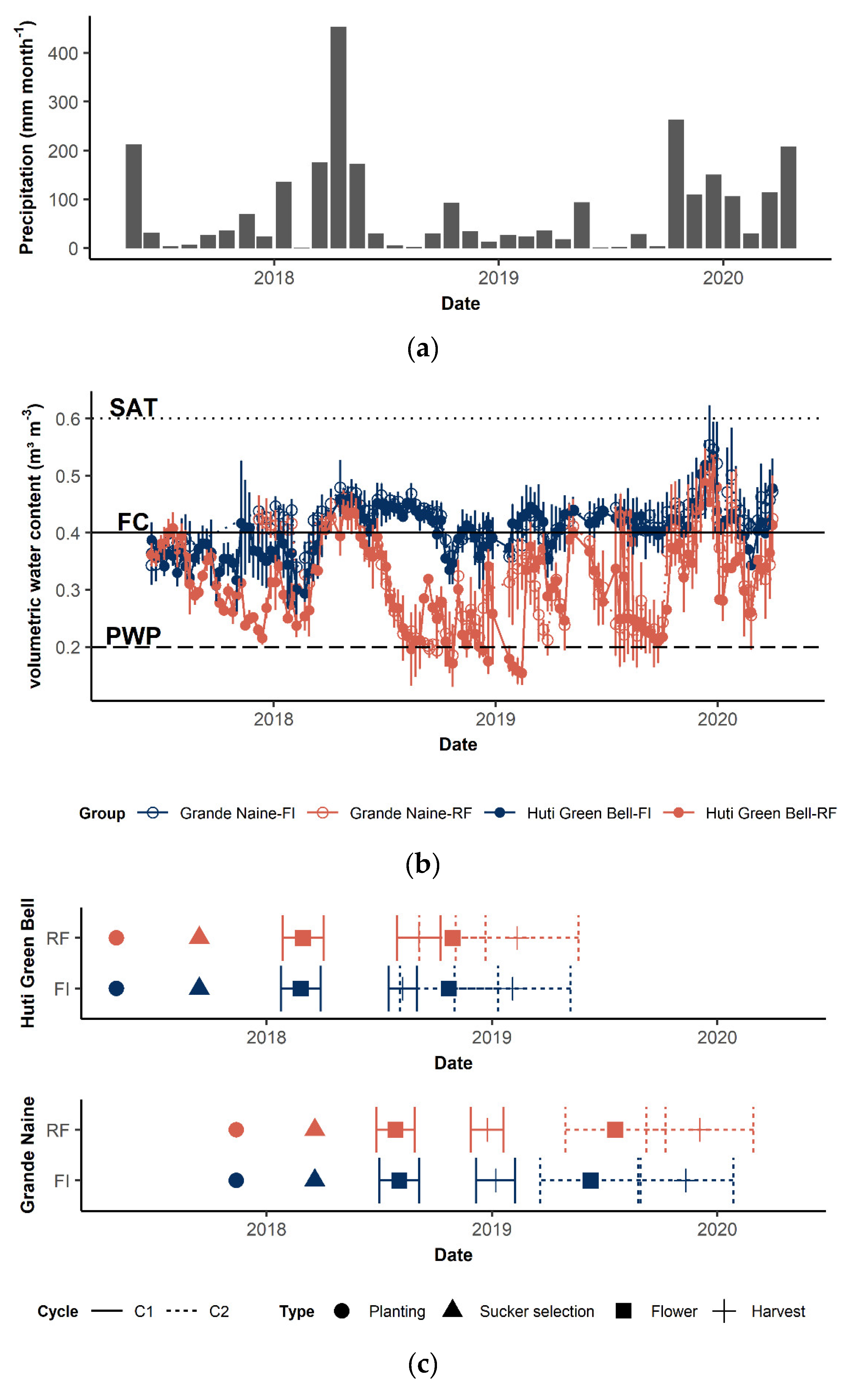
3.1.1. Difference in Moisture

The onset of soil moisture differences differed between experiments (Figure 1b), due to differences in planting time (Figure 1c) resulting in rainfall periods affecting plants at a different growth stages (Figure 1a–c). In HG, moisture differences became significant during the vegetative stage of C1 onwards, whilst for GN, moisture differences occurred from the approximate onset of flower emergence in C1 (Figure 1b,c) [25]. This is reflected in the ratio between water and ET0 between planting and flowering (RPF) (Table 2). RPF differed significantly between treatments in both cycles and cultivars (p < 0.05). RPF during HG C1 differed between treatments, but remained suboptimal for both FI (0.743 ± 0.03) and RF (0.638 ± 0.0404), indicating stressed vegetative growth. RPF during GN C1 was optimal in both FI (1.44 ± 0.0213) and RF (1.26 ± 0.0448), indicating non stressed vegetative growth until flowering.
During bunch development, RFH differed significantly between treatments in all cycles and cultivars (p < 0.05). RFH was always optimal or close to 1 in FI, but not in RF except in HG-C1 where RF plants developed bunches during the rainy season (RFH = 1.47 ± 0.182). Contrastingly, GN C1 plants developed bunches during the dry season as shown by RFH of 0.329 (±0.0239) for RF C1.

3.1.2. Effect on Phenology

Under increased soil moisture stress, a delay in banana phenology occurred, but severity of delay differed between cultivars and cycles. In HG, flowering differences were small (4 days) in C1, and not significant in C2. In GN, differences in DTF were more pronounced. RF plants flowered on average 6 days earlier in C1. In contrast, FI plants flowered on average 40 days earlier in C2 (p < 0.05).
Differences in harvest date (DTH) were more pronounced. In HG, FI plants were harvested 37 and 76 days earlier in C1 and C2, respectively. In GN, there was no difference in C1 (p > 0.05) but harvest occurred 34 days earlier in C2 FI plants (p < 0.05) (Table 2).

3.1.3. Effect on Vegetative Growth

Vegetative growth was affected significantly by irrigation (Table 2). FI increased parameters H, Gbase, and Vpseudo significantly, except for GN C1 (p = 0.24 for H, p = 0.55 for Gbase) as these developed under RPF > 1 until flowering of C1 (Table 2). Correspondingly, FI increased vegetative biomass ABGVD at harvest (p < 0.05) (Table 2).

3.1.4. Effect on Bunch Growth

Bunch growth was also significantly affected by irrigation (Table 2). BunchF differences under irrigation were reflected in measured bunch parameters (Table 2). In HG, Nhand was increased in FI in C1 (p = 2.7 × 10⁻⁴), but similar in C2 (p = 0.83). Nfinger increased in both cycles, and fingers were also bigger (Vfinger) under irrigation (p < 0.05). This resulted in significant increased bunchF under irrigation in C1 and C2 (p < 0.05).
In GN, Nhand was similar in both cycles between FI and RF (Table 2), but Nfinger increased under FI in C2 (p = 4.4 × 10⁻⁴) (Table 2). Large differences were obtained during bunch filling, as FingerF and Vfinger increased under FI in both cycles (p < 0.05). Differences between RF and FI occurred due to differential soil moisture during bunch filling (RFH = 0.333 in RF C1) from C1 onwards (Figure 1a).

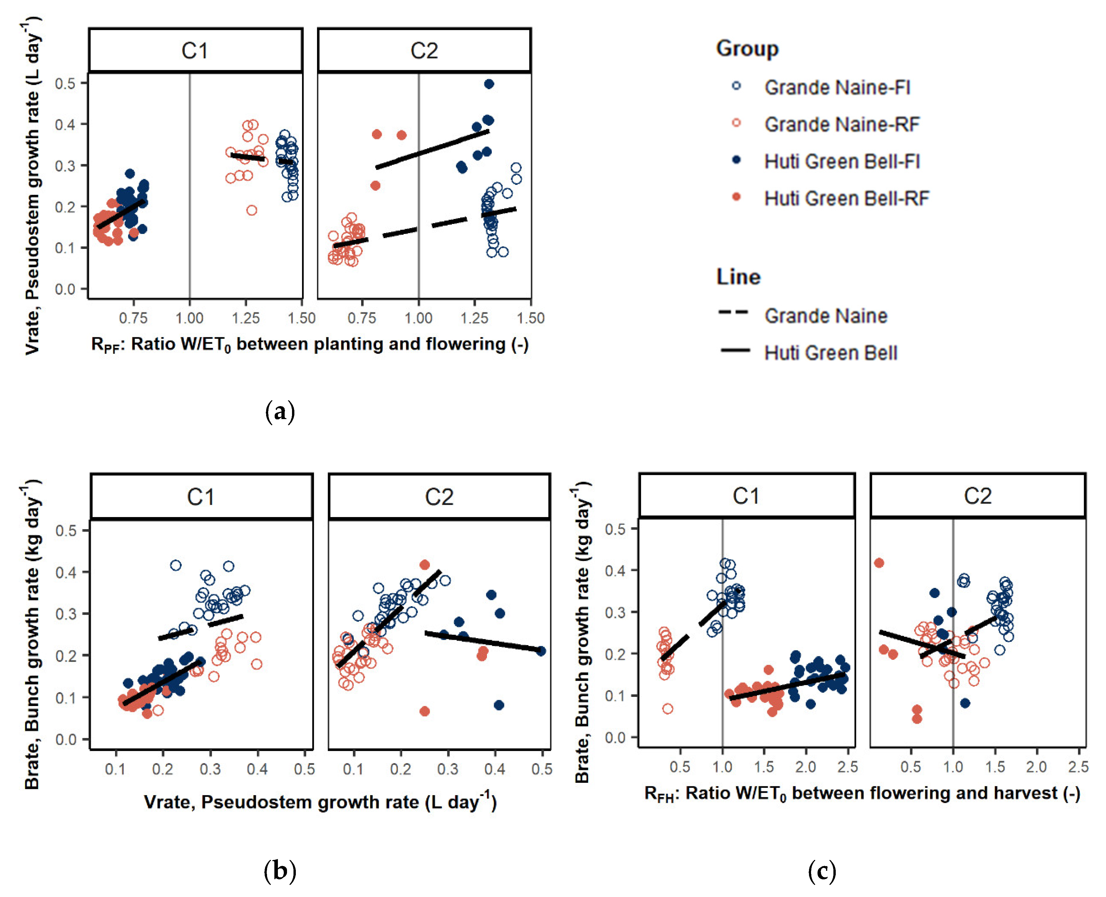
3.1.5. Effect on Growth Rates

Combining phenology and growth parameters shows growth speeds (Vrate and Brate) of plants differed significantly between the treatments (Figure 2 and Table 3). Moisture (RPF) had a significant effect on growth rates of the pseudostem (Vrate), except in GN-C1 as these plants all developed under optimal conditions (RPF > 1). In all other groups, RPF had a significant (p < 0.05) positive effect on Vrate in HG and GN. Both Vrate and moisture after flowering (RFH) had a significant effect on bunch growth rates (Brate) (Figure 2 and Table 5).
Generally, an increase in Vrate led to an increase in Brate, except for HG-C2. Vrate on its own does not fully explain the bunch growth rate (Table 5) as coefficients for RFH are significant in several models. This is shown clearly in GN–C1, as Vrate in FI plants is smaller, but bunch growth rates are significantly larger (p < 0.05) (Table 2). Inclusion of RFH proves necessary for correctly assessing Brate.

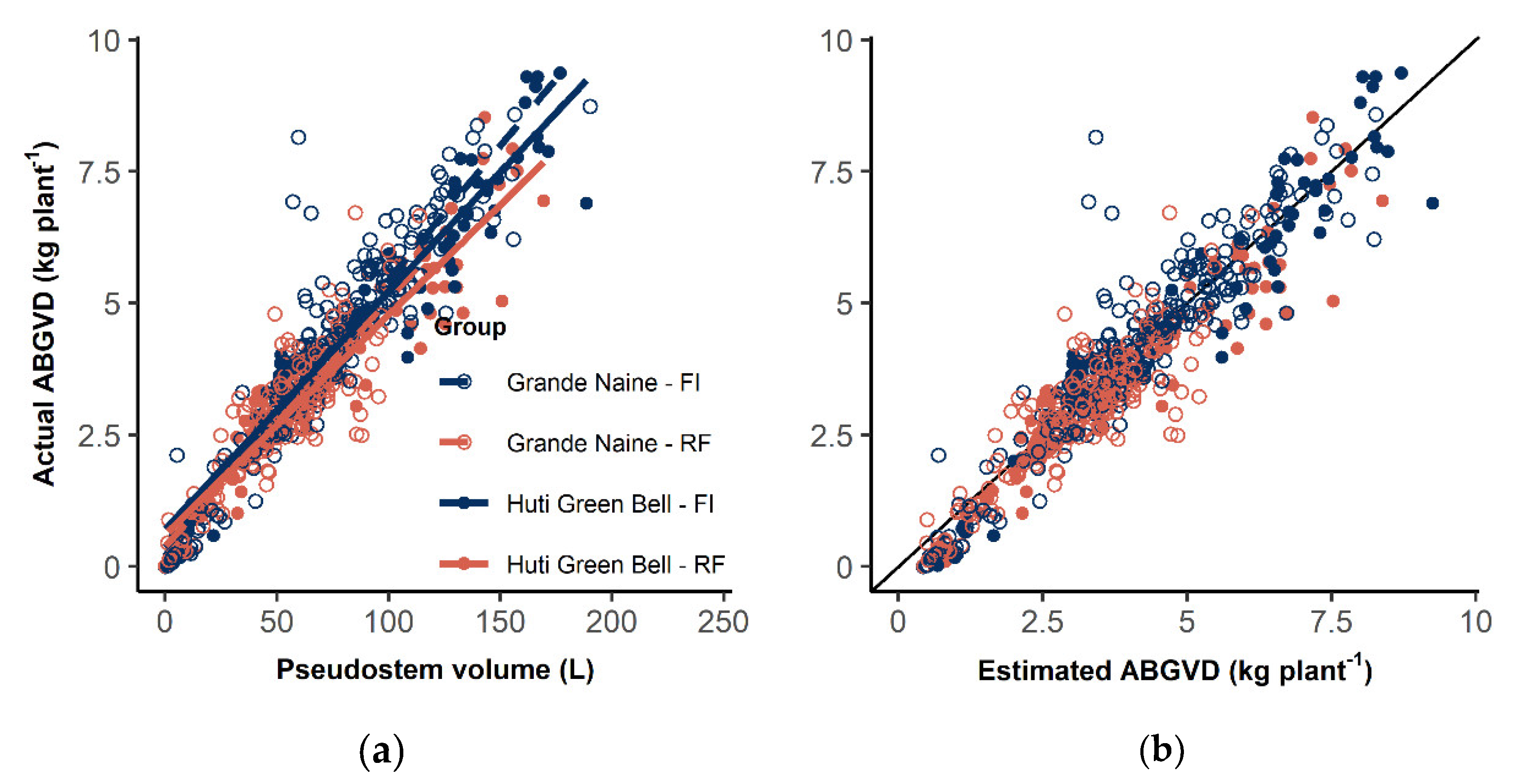
3.2. Aboveground Vegetative Dry Matter Estimation

Vpseudo was linearly related to ABGVD in both HG and GN (Figure 3), and to all its components (leafD, petioleD, and pseudostemD) (Figure S4). VIFs higher than 5 (indicating collinearity) were not found in our models (Table 4).
Models using only Vpseudo as a predictor already had a good model fit in HG and GN (RRMSE = 0.14) (Table 4). Lm.1 was the best model in terms of goodness of fit, and practicality, and was used for creating pooled and specific regression models (Table 5).
Specific FI and RF models for ABGVD showed overlapping 95%CI model coefficients for intercept and slope in both HG and GN (Table 5), but coefficients were different between treatments using the ANCOVA method. For HG, the intercept was reduced in the RF model by 0.32 (p = 8.25 × 10⁻¹⁴), and the slope was very slightly reduced by 5 × 10⁻³ (p = 0.014). For GN, there was no effect on the intercept (p = 0.13) and the slope was reduced by 6.07 × 10−03 (p = 4.46 × 10⁻³) in RF (Figure 3 and Table 5).
Comparing predictions of the FI models with RF models, led to bias% of −92.1% (HG) and −81.9% (GN) for FI plants and bias% of −44.6% (HG) and −41.4.0% (GN) for RF plants. Both FI and RF plants were overestimated. Small plants (<25L) were overestimated in small absolute terms (<1 kg DM plant−1), but as bias% calculates the relative deviation, these had a large effect on the overall bias%. Recalculating bias% after removal of the smaller plant (<25L) led to bias% of 2.07% (HG) and −1.48 (GN) in FI, and bias% of −7.26% (HG) and −10.1% (GN) in RF. Plants <25 L were overestimated in both FI and RF (in small absolute terms), but plants >25 L were only overestimated in RF.
Comparison of cultivar FI models showed 95%CI model coefficients overlapped for intercept and slope (Table 5) but models were distinctly different in intercept (p = 0.01) and slope (p = 8.89 × 10⁻⁴) following ANCOVA.
As 95%CI for coefficients overlapped between treatments and cultivars, the differences although significant, may be small in practice. Pooling data from both cultivars and treatments (n = 700) and performing the regression on this pooled data led to a good model fit (R2adj = 0.90, RRMSE = 0.18), using Vpseudo as predictor (Table 5).
The model for estimating ABGVD in HG and GN becomes:
ABGVD = 0.33 + 6.02 × 10 2 × Vpseudo ;   HG   and   GN   combined
with ABGVD, aboveground vegetative dry matter (kg DM plant−1) and Vpseudo, pseudostem volume (L).

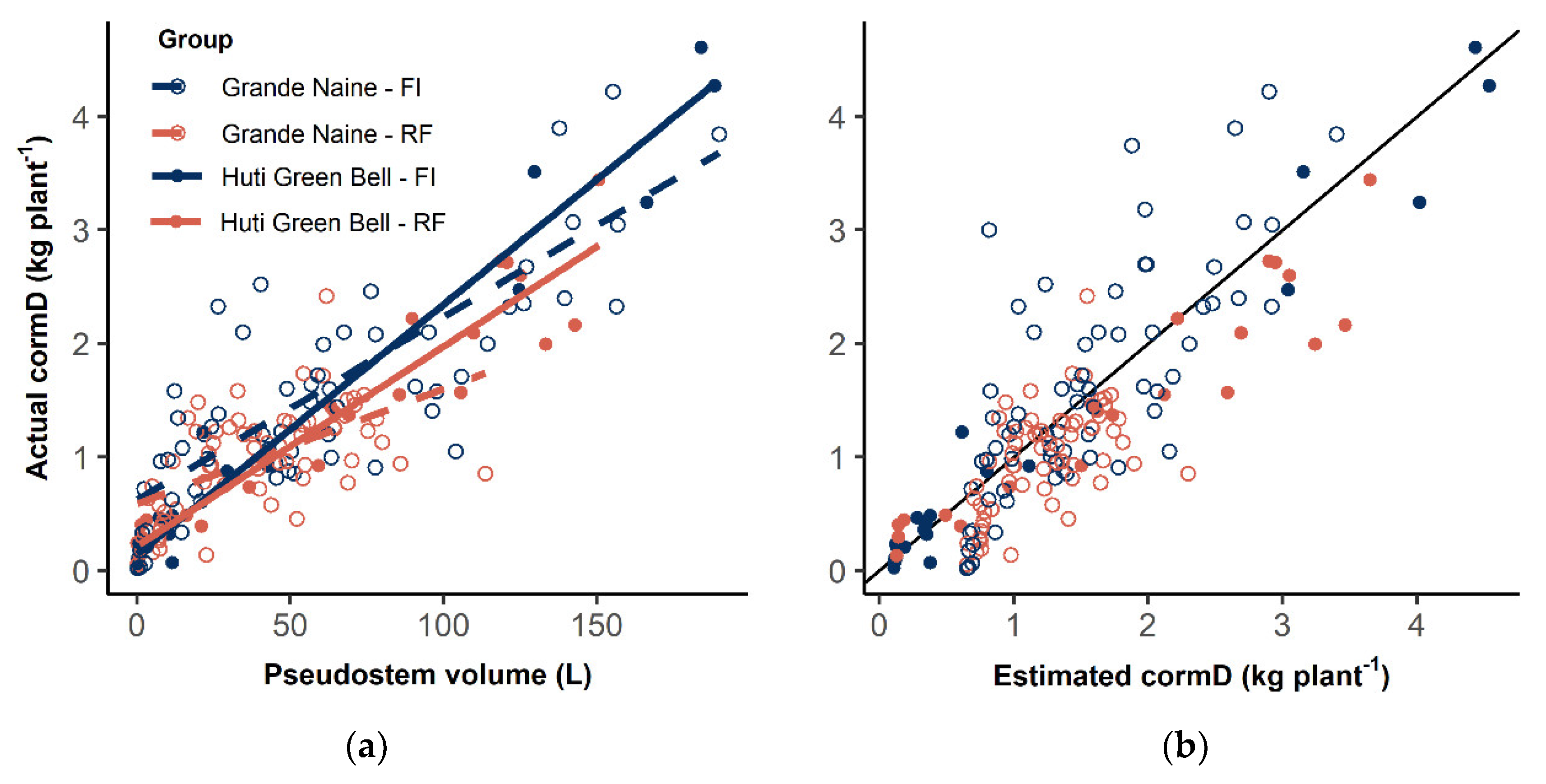
3.3. Corm Dry Matter Estimation

Vpseudo was linearly related to cormD in both HG and GN (Figure 4). VIFs higher than 5 were not found in the cormD models.
Models with only Vpseudo and LAI as predictors for cormD led to a fair model performance for HG (RRMSE = 0.22) but poor model performance for GN (RRMSE = 0.34) (Table 4). Lm.1 was the best model in terms of goodness of fit and used for creating pooled and specific regression models (Table 5).
Specific FI and RF models revealed 95%CI of coefficients overlapped for both HG and GN (Table 4), but coefficients were significantly different between treatments in both HG and GN using the ANCOVA method. For HG, RF reduced the slope by 4.01 × 10⁻³ (p = 5.18 × 10⁻³), had no effect on the intercept (p = 0.09) (Figure 4, Table 5). For GN, RF reduced the intercept by 0.01 (p = 2.22 × 10⁻⁵) and the slope by 5.22 × 10⁻³ (p = 7.59 × 10⁻⁴) (Figure 3). Due to overlap of 95% CI, differences were not so pronounced.
All models for cormD (Table 4 and Table 5) were suboptimal given the fair to poor RRMSE values, and the large variation around the 1/1 line (Figure 4). Therefore, specific model differences may not be correct, and care should be taken.
Using the specific FI regression models led to a bias% of −54.5% (HG) and −156% (GN) for FI plants, and bias% of −13.2% (HG) and −73.2% (GN) for RF plants. Models overestimated the cormD in both treatments and cultivars. Overestimation occurred again through the influence of smaller plants. Recounting bias% after removal of smaller plants led to a bias% of −3.78% (HG) and −11.0% (GN) for FI compared to −23.6% (HG) and −39.2% (GN) for RF. Thereby, the RF plants were overestimated more strongly compared to the FI plants. In general, models overestimated small plants (<25 L), whereas bigger plants show no overestimation in HG FI, show a slight overestimation in GN FI plants, and show a large overestimation in RF plants of both cultivars.
Cultivar FI models were also different as 95%CI coefficients did not overlap, and following ANCOVA, HG model intercepts were reduced (p = 1.77 × 10⁻⁴) and slopes increased (p = 0.05) compared to GN. The best models for estimating cormD for HG and GN became
cormD = 0.13 + 2.24 × 10 2 × Vpseudo ;   HG
cormD = 0.62 + 1.08 × 10 2 × Vpseudo ;   GN
with cormD, corm dry matter (kg DM plant−1), and Vpseudo, the pseudostem volume (L).

3.4. Bunch Weight Forecast

ABGVD was significantly positively correlated to bunchF (p < 0.05) with R2adj of 0.73 (FI) and 0.65 (RF) for HG, and R2adj of 0.61 (FI) and 0.54 (RF) for GN. Similarly, Vpseudo, Flower was linearly related to bunchF at harvest (Figure 5). VIFs higher than 5 were not identified in the bunch models.
Models containing only early bunch data (lm.1 to lm.7) had RRMSE values ranging from 0.12 to 0.25 (HG) and 0.13 to 0.2 (GN) indicating good model fit (Table 4). Inclusion of data on sucker size (Vpseudo,flowerS) did not improve the RRMSE of the models (lm. 6 to lm.7) compared to models with only Vpseudo,flower (lm.1). Inclusion of data collected at later stages (lm.8 to lm.11) improved model fits as RRMSE values reduced and R2adj increased. To allow for earliest bunch estimation, model containing Vpseudo, Flower (lm.1) were retained for both HG (R2adj = 0.70, RRMSE = 0.12) and GN (R2adj = 0.43, RRMSE = 0.15).
Pooled and specific regression models proved different between treatments in both HG and GN (p < 0.01) (Table 5). Model coefficients did not show overlap in the 95%CI. For HG, RF led to a significantly lower intercept (ANCOVA, p = 7.18 × 10⁻¹²), whilst slopes remained similar (ANCOVA, p = 0.38). For GN, the intercept and slope were different between treatments (p < 0.05) leading to widely different relationships with Vpseudo, Flower (Figure 4, Table 4).
Using the specific FI regression models to estimate bunchF for both FI and RF plants, led to a significant overestimation of RF bunches in both HG and GN (Figure 5). The bias% for FI plants was −2.31% (HG) and −1.74% (GN) and the bias% of the RF plants was −28.0% (HG) and −24.1% (GN). Therefore, using FI models significantly overestimated the RF plants.
The specific models were also different between the cultivars (p < 0.01, Figure 5 and Table 5). Models for optimal bunch weights (FI conditions) became:
bunchF = 0.13 + 2.24 × 10 2 × V pseudo , flower ;   HG-FI
bunchF = 0.62 + 1.08 × 10 2 × V pseudo , flower ;   GN-FI
with bunchF being fresh bunch weight (kg plant−1), and Vpseudo,flower being the pseudostem volume (L) at flowering.

4. Discussion

4.1. Effect of Moisture on Vegetative and Bunch Growth

Irrigation resulted in significant soil moisture differences (Figure 1b) affecting phenology, vegetative growth, and bunch growth (Table 2). Drought in banana induces stomatal closure, reducing transpiration and photosynthesis which reduces leaf area, leaf emission rate, and vegetative growth in general [18,25,35,36,37]. Drought during flower initiation may reduce Nhand per bunch and Nfinger per hand [28], whereas drought after flower initiation results in suboptimal fruit filling [38].
HG plants already experienced different moisture regimes during C1 vegetative growth and thereby differed between FI and RF in both vegetative and bunch parameters (Table 2). GN plants developed under optimal conditions (RPF > 1) until flower emergence of C1 [25], thereby FI and RF plants of C1 did not differ in Vpseudo, Nhand, and Nfinger (Table 2), parameters that are determined during the vegetative stage. Differences in RFH from C1 flowering onward (Figure 1b and Table 2) led to differences in ABGVD, fingerF, Vfinger, Ratiofinger, and bunchF at harvest.
Phenology was delayed under drought depending on the severity of moisture deficit. Differences in flowering (DTF) remained small, but differences in harvest (DTH) were very pronounced with FI plants being harvested much earlier in both cycles and cultivars (Table 2). Flowering of GN C1 occurred 6 days earlier in RF plants, but RPF of both treatments was bigger than 1, so RF plants developed optimally until flowering. After flower emergence, RFH ratios in RF plants were significantly lower than 1 (0.329 ± 0.0239) delaying harvest. Differences in DTF and DTH increased in C2, as plants of C2 developed under more significant moisture stress for GN (Table 2). Environmental stress due to suboptimal soil moisture has been shown to delay floral development and increase bunch filling duration in banana plants [18,39,40].
Combining absolute growth and phenology, showed effects of moisture on pseudostem (Vrate) and bunch (Brate) growth rates (Table 3, Figure 2). Vrate was influenced by RPF (p < 0.05, Table 3), although effects differ due to the size of RPF. If RPF > 1, moisture covers the evaporative demand as shown in GN-C1, where Vrate was not influenced by RPF as RPF was optimal for both RF and FI (Table 3). Only when RPF was less than 1, Vrate seemed to be negatively affected (Figure 2 and Table 3). In order to achieve fast vegetative growth rates, RPF should remain above 1.
The effect of Vrate on Brate was significant (Table 3), as faster Vrate resulted in increased Brate (Figure 2b). Moisture after flowering (RFH) also influences Brate significantly (Table 3, Figure 2c). RFH needs to be bigger or close to 1 to ensure optimal bunch filling (Figure 2 and Table 3). Within cycles and cultivars, we see that an increased RFH has the bigger Brate for GN and HG (except HG C2).
Moisture deficit thereby has a double effect on bunch growth. Firstly, moisture deficits during the vegetative stage (RPF < 1) reduce the vegetative growth of the plant (Vrate), which reduces the Brate. During bunch filling, previously stored nutrients are translocated to fill the bunch [2,3,4,5]. Less vegetative biomass thereby indicates less translocation potential. Secondly, moisture deficits during the bunch filling stage (RFH < 1) affect translocation and bunch filling [18,39], resulting in a reduced Brate. Both stages are important in the eventual outcome of the bunch weight. In order to achieve optimal growth for the pseudostem and the bunch, added moisture amounts should be compared to evaporative demands of the atmosphere. If the added moisture amounts are significantly less than the reference evapotranspiration (R < 1), moisture needs to be added to ensure optimal growth.

4.2. ABGVD Estimation from Non-Destructive Observations

Vpseudo was significantly linearly correlated to the ABGVD (Figure 3), and a good predictor for ABGVD in both HG and GN (RRMSE of 0.14) (Table 4). Height, girth, and diameters (components for volume estimation) are often used in biomass regression [7]. In trees, height and diameter at breast height are significantly correlated to biomass of a stand [7,41,42]. Negash et al. [8] found girth at base to be the best predictor for aboveground biomass estimation (R2 = 0.77–0.98) in Enset. Nyombi et al. [5] found girth at base to be the best predictor in development-stage specific regressions (R2 = 0.79–0.99), but height to be the best predictor of ABGVD when pooling the data across development stages (R2 = 0.98). Combining height and girth leads to a parameter describing the pseudostem (volume) in three dimensions, without leading to high co-linearity when keeping both parameters in the model [7]. Vpseudo is linked to all components of aboveground biomass (pseudostem, leaves, and petioles) in our field (Figure S4). The pseudostem is composed of tightly compacted leaf sheaths, which result from previous cumulative leaf formation. Vpseudo was therefore also correlated to the petiole and leaf mass in our field (Figure S4) [39]. However, the number of leaves and petioles at a given time are also affected by management practices (e.g., pruning) and stress conditions, indicating correlations can differ in other plantations.
Even though Vpseudo was affected by soil moisture deficit, the relationship between Vpseudo and ABGVD was not influenced strongly. Specific regression models for ABGVD between treatment and cultivar differed according to ANCOVA (p < 0.05) (Table 4), but differences were small as 95%CI for model coefficients overlapped. Pooling cultivar and treatment data led to a good model fit (R2adj 0.90 and RRMSE 0.18, Table 5) indicating a single ABGVD model based on Vpseudo can be used (Equation (2)).
Perhaps stress was not marked enough for ABGVD plasticity under drought as average bunches in RF plots ranged from 19.6 to 24.4 kg plant−1 in HG, and from 33.2 to 33.3 kg plant−1 for GN, which are considered good yields. Nyombi et al. [5] had irrigated yields for EAHB cv. Mbwazirume ranging from 20 to 40 kg plant−1, whilst Wairegi et al. [9] showed yields for different rainfed EAHB cultivars from on farm visits ranging from 2–60 kg plant−1. Our yields are therefore higher compared to their lower range, hence less stress was present.
Models did overestimate small plants (<25L). This overestimation might be a characteristic of the model, as the intercept was not forced through zero during modelling as this may lead to poorer goodness of fit characteristics [43]. At Vpseudo zero, there is an overestimation of 0.54 kg DM plant−1 (HG) and 0.22 kg DM plant−1 (GN), which are small absolute DM values, but with a large influence on the total bias%. Removing smaller plants reduced bias%. Overestimation of small plants could also be due to the growing behavior of suckers. Small suckers have scale and lanceolate leaves but produce foliage leaves at approx. 1.5 m height [2,44]. Shading results in improved partitioning to aboveground structures [45] and leads to an increase in pseudostem growth to faster reach sunlight. Therefore, small plants might have a lower pseudostem density (kg DM volume−1), leading to an overestimation when presuming their density to be similar to bigger plants. Another possibility is that all smaller plants are in the vegetative stage. Nyombi et al. [5] found that vegetative aboveground biomass models differ according to plant growth stage (vegetative, flowering, or harvest). Plants in the vegetative stage had a lower ABGVD compared to plants at flowering and harvest with similar girths and heights. Pooling the data across these plant growth stages might have led to this overestimation caused by small plants, but the overestimation is small in absolute terms (<1 kg DM plant−1), still warranting the use of a general regression model as this is more practical. The general regression model to use for ABGVD estimation to be used is given in Equation (2).

4.3. CormD Estimation from Non-Destructive Observations

Vpseudo was linearly correlated to the belowground cormD (Figure 4). CormD models based on Vpseudo ranged from fair in HG (RRMSE = 0.24) to poor in GN (RRMSE = 0.33) (Table 4), making Vpseudo less suitable for cormD estimation. Nyombi et al. [5] found good exponential relationships between pseudostem girth at base and cormD (R2 = 0.59–0.98) but cormD in their field ranged between 0–0.40 kg plant−1, which seems low compared to our cormD values ranging from 0.09–4.27 kg plant−1. Negash et al. [8] found good correlations between belowground biomass (corm and adventitious roots) and diameter at base for Enset (R2 = 0.75), but found no such correlation with height (R2 = 0.23–0.27). Creating power models with radius at base instead of Vpseudo did not improve model fits for cormD in both HG (RRMSE = 0.38) and GN (RRMSE = 0.41) (data not shown).
Using aboveground characteristics to describe a belowground structure has shortcomings. Parameters relating to corm dimensions (e.g., corm height and girth) are expected to considerably improve the cormD estimation, but in order to estimate these the corm needs to be excavated. Corm dimensions also vary in diameter and height with plant growth phase (vegetative, flowering, harvest) and whether the plant is in the first or second cycle [2]. The corm is a storage organ whose reserves are used for fruit growth and sucker development, whereby bunch development stage, size and the amount of produced suckers also play a role in corm biomass [2]. In our field, the variation of cormD with Vpseudo increased with cycle, thereby partitioning models in terms of cycle or plant growth phase (vegetative, flowering, harvest) might significantly improve the model. Nyombi et al. [5] found growth stage specific allometric relationships for cormD, whereby R2 reduced from the vegetative (0.98) to the harvest phase (0.57), signifying increased variation with increasing growth stage.
The comparison of specific models across treatments revealed irrigation effects to be significant (ANCOVA, p < 0.05), but as 95%CI intervals overlap between specific treatment models, differences were not very pronounced (Table 4). Pooled data per cultivar did not increase RRMSE much, leading to the conclusion that cormD models are similar among RF and FI. It seems that at a given Vpseudo, cormD will be higher in FI than in RF plants, but given the suboptimal nature of models based on Vpseudo we cannot be certain of the water stress effects on corm allometry. The biomass of the underground corm structure is too variable to accurately predict based on aboveground vegetative characteristics alone, and care must be taken using these relationships.

4.4. Bunch Yield Forecast

Vegetative growth (Vrate) was linked to bunch growth in our field (Brate) (Figure 2 and Table 3). Others have also shown pseudostem size significantly correlates with bunch weights: R2 = 0.63–0.85 [4], R2 = 0.66 [9], R2 = 0.57–0.7 [5], R2 = 0.97–0.98 [10]. The pseudostem size relates to bunch filling potential as assimilates are translocated during the bunch filling stage [2,4,5,46] even across ratoon plants [47]. High yields are linked to vigorous early plant growth in plantain [3].
As such, stepwise regression revealed Vpseudo, Flower to be the most important predictor of bunchF compared to other regression models (R2adj of 0.7 for HG and 0.43 for GN; RRMSE of 0.12 for HG and 0.15 for GN) (Table 4). Inclusion of bunch related predictors (Nfinger, Nhand, Vfinger) improved model fits as R2adj increased (0.81 for HG and 0.78 for GN) and RRMSE decreased (0.1 for both HG and GN lm.11) (Table 5). The more parameters were included closer to bunch harvest, the better the prediction. Practically, using Vpseudo,flower as a predictor for bunchF already led to good model performance in both HG and GN FI models (RRMSE 0.13–0.14).
Bunch models based on Vpseudo,flower were very different between FI and RF, as 95%CI did not overlap and following ANCOVA(p < 0.05). FI models performed better (RRMSE 0.13 for HG, 0.14 for GN) than RF models (RRMSE 0.15 for HG, 0.23 for GN).
These different relationships between bunchF and Vpseudo,flower under drought follow differences in bunch characteristics under RF vs. FI conditions (Table 2). Drought during flower initiation may reduce Nhand and Nfinger whereas drought during bunch filling results in suboptimal fruit filling (Vfinger) [2,18,38]. Moisture regimes at and after flowering are thereby crucial in determining actual bunch weights in the field, but these are not reflected in Vpseudo,Flower. Up until flower emergence, GN plants of C1 developed optimally in both treatments (RPF > 1, Table 2) [25]. Height and girth (Vpseudo), Nfinger and Nhand did not differ at flowering (p > 0.05), whilst bunchF, finger, and Vfinger did differ between FI and RF at harvest (p < 0.05) (Table 2). Weight and size of the fingers determined the bunch weights. Plants of similar Vpseudo,flower subjected to different environments (RFH) after flowering (e.g., GN C1) will thereby have different bunchF at harvest, changing relationships between these parameters.
For accurate bunch weight estimation, bunch characteristics need to be included [9,12]. Our models improved (RRMSE became lower) when bunch parameters were included, but this no longer allows forecasting of bunch weights as bunch characteristics (e.g., Vfinger) change until harvest.
Our FI models can be used to forecast bunch weights if plants developed without stress from flowering onwards (as RFH >1 in FI). Forecasting of bunchF based on Vpseudo,Flower allows to estimate bunch ‘potential’ weights as in Equations (4) and (5).
To estimate ‘actual’ bunch weights, the environmental effects during bunch filling need to be incorporated either directly (e.g., as RFH) or indirectly (e.g., effect of RFH on Vfinger).
The large phenotypical differences between HG and GN plants, also led to significantly different bunch weight regression curves for cultivars (p < 0.05). However, as cultivars were planted at a different time, differences in planting might confound differences in cultivars and we should not compare these cultivars with each other. Nyombi [5] found different allometric relationships for bunch weight for two EAHB cv Mbwazirume and Kisansa. Wairegi et al. [9] proposed the use of a general banana regression curve for estimation of EAHB bunch yields, but their results showed cultivar specific curves were characterized by lower overall variances and increased model fits. Their cultivar specific curves were similar but were significantly different in model parameters. Our results support the statement that even genetically close cultivars have different phenotypical characteristics [30].
A bunch forecast model based on Vpseudo,flower needs to include additional parameters that relate to environment conditions after flowering to properly work.

5. Conclusions

Irrigation and corresponding soil moisture differences had a significant effect in both HG and GN, reducing vegetative and bunch growth, and delaying phenology under RF conditions. Of the effected parameters, Vpseudo seems a promising indicator as it is linked to both vegetative growth and bunch growth rates. The universal nature of Vpseudo as a regression parameter between the two cultivars is more valuable for future allometric studies than girth or height alone.
Allometric relationships for vegetative biomass (ABGVD and cormD) were not strongly affected by irrigation as 95% CI overlapped between FI and RF models indicating a single allometric model can be used across RF and FI plants for vegetative biomass estimation. Models did also not differ much between our phenotypically very different cultivars for ABGVD, hinting Vpseudo models can be used across a range of cultivars. Vpseudo did not prove sufficient to estimate cormD reliably, as a lot of variation remained in the underground biomass. Aboveground characteristics are therefore lacking to estimate belowground structures. For better estimation of belowground vegetative biomass, components relating to the corm dimensions can be added although these are more difficult to measure. This research shows the potential for non-destructive vegetative biomass monitoring at the field scale, and shows soil moisture to not affect vegetative allometry significantly. As biomass over time often underlies crop simulation models, this is especially useful for researchers wanting to calculate biomass in the field for calibrating such models without destroying plants.
Bunch weight (bunchF) forecasting models based on Vpseudo at flowering were significantly different between FI and RF, showing bunch weights cannot be estimated on vegetative parameters only, without including information on stress during bunch filling or bunch components. Both vegetative growth (Vrate) and moisture during bunch filling (RFH) determine bunch growth rates. Our FI models do allow prediction of bunch weights under optimal conditions after flowering (RFH≥1) and can be used to forecast bunch weight potentials based on Vpseudo at flowering.

Supplementary Materials

The following are available online at https://www.mdpi.com/2073-4395/10/9/1435/s1. Figure S1: Diagram of experimental design for experiment 1 and experiment 2; Figure S2: Initial plant heights for planting materials (a) Initial plant height for Huti Green Bell in cycle 1 (C1) (b) Initial plant height for Grande Naine in C1, (c) Initial plant height for Huti Green Bell in cycle 2 (C2)and (d) Initial plant height for Grande Naine in C2; Figure S3: Growth of pseudostem (L) over time in Grande Naine of individual plants in cycle 2 (C2). Dots indicate actual growing measurements, lines indicate local non-parametric regression curves of individual plants under full irrigation (FI) and Rainfed (RF). Red dots indicate the intersection of the regression curves with the date of flowering of C2 and show the interpolated VpseudoFlower; Figure S4: Components of aboveground vegetative dry biomass (ABGVD, kg plant−1). (a) Leaf dry weight (leafD, kg plant−1) versus pseudostem volume (L); (b) Petiole dry weight (petD, kg plant−1) versus pseudostem volume (L); (c) Pseudostem dry weight (pseudostemD, kg plant−1) versus pseudostem (L). Used regression models in (a), (b) and (c) were specific models for treatment and cultivar using pseudostem volume as predictor. (d) Ratio between sum of leafD and petioleD to pseudostemD. FI notes full irrigation, RF notes rainfed. Table S1: Dry matter (DM, g dry matter g fresh weight−1) (mean and sd) of the plant organs obtained in the field trial. Moisture contents were determined from subsamples of plant organs taken at harvest from the different cycles. Treatment differences were not significant (p < 0.05), leading to the pooling of data across the treatments (FI: full irrigation and RF: rainfed) per cycle (C1, C2 and C3) to obtain a dry matter percentage per organ per cycle.

Author Contributions

Conceptualization: B.S., J.D., A.B., P.A.N., R.S.; Data curation: B.S.; Formal analysis: B.S.; Funding acquisition B.S., J.D., R.S; Investigation: B.S., S.B.; Methodology: B.S., J.D., R.S.; Project administration: B.S., J.D., R.S.; Resources: B.S., J.D., A.B., P.A.N., R.S.; Software: B.S.; Supervision J.D., A.B., P.A.N., R.S.; Writing—original draft: B.S., J.D., A.B., B.S.; Writing—review and editing: B.S., J.D., R.S.; Visualization: B.S. All authors have read and agreed to the published version of the manuscript.

Funding

This research was funded by the Belgian VLIR-UOS VLADOC scholarship, grant number NDOC2016PR0009. The authors are also grateful to all donors who supported this work through their contributions to the CGIAR Fund (https://www.cgiar.org/funders/) and in particular to the CGIAR Research Program for Roots, Tubers, and Bananas (CRP-RTB).

Acknowledgments

This study was conducted at the joint research farm of the Nelson Mandela African Institution of Science and Technology (NM-AIST) and the International Institute of Tropical Agriculture (IITA), hence many people were involved. We thank the many people involved in fieldwork and technical assistance: Erick Wangaely, Salim Ramadhani, and Joshua Jackson for the maintenance of the field; Hassan Mduma and Veronica Massawe for their practical guidance and Scola Ponera and Joyce Rugakingila for administrative support.

Conflicts of Interest

The authors declare no conflict of interest.

Abbreviations

Abbreviated growth parameters are found in Table 1.
C1, C2, and C3Cycle 1, 2, and 3
EAHBEast African Highland Banana
FIFull irrigation
GNCavendish–Grande Naine
HGMchare-Huti Green Bell
IITAInternational Institute of Tropical Agriculture
NM-AISTNelson Mandela African Institution of Science and Technology
RFRainfed
RFHRatio of moisture received to ET0 between flowering and harvest
RPFRatio of moisture received to ET0 between planting and flowering
RPHRatio of moisture received to ET0 between planting and harvest
WLSWeighted least squares regression

References

  1. FAOSTAT. Banana And Plantain Production Data. Available online: http://www.fao.org/faostat/en/#data/ (accessed on 14 August 2020).
  2. Robinson, J.C.; Galán Saúco, V. Bananas and Plantains, 2nd ed.; Longmans: London, UK, 2010; ISBN 9781845936587. [Google Scholar]
  3. Swennen, R.; Langhe, E.D. Growth Parameters of Yield of Plantain (Musa cv. AAB). Ann. Bot. 1985, 197–204, 197–204. [Google Scholar] [CrossRef]
  4. Mukasa, H.H.; Ocan, D.; Rubaihayo, P.R.; Blomme, G. Relationships between bunch weight and plant growth characteristics of Musa spp. assessed at farm level. MusAfrica 2005, 16, 2–3. [Google Scholar]
  5. Nyombi, K.; Van Asten, P.J.A.; Leffelaar, P.A.; Corbeels, M.; Kaizzi, C.K.; Giller, K.E. Allometric growth relationships of East Africa highland bananas (Musa AAA-EAHB) cv. Kisansa and Mbwazirume. Ann. Appl. Biol. 2009, 155, 403–418. [Google Scholar] [CrossRef]
  6. Niklas, K.J. Plant allometry: Is there a grand unifying theory? Biol. Rev. 2004, 79, 871–889. [Google Scholar] [CrossRef] [PubMed]
  7. Picard, N.; Saint-André, L.; Henry, M. Manual for Building Tree Volume and Biomass Allometric Equations: From Field Measurement to Prediction; Food and Agricultural Organization of the United Nations, Rome, and Centre de Coopération Internationale en Recherche Agronomique pour le Développement: Rome, Italy, 2012. [Google Scholar]
  8. Negash, M.; Starr, M.; Kanninen, M. Allometric equations for biomass estimation of Enset (Ensete ventricosum) grown in indigenous agroforestry systems in the Rift Valley escarpment of southern-eastern Ethiopia. Agrofor. Syst. 2013, 571–581. [Google Scholar] [CrossRef]
  9. Wairegi, L.W.I.; van Asten, P.J.A.; Tenywa, M.; Bekunda, M. Quantifying bunch weights of the East African Highland bananas (Musa spp. AAA-EA) using non-destructive field observations. Sci. Hortic. 2009, 121, 63–72. [Google Scholar] [CrossRef]
  10. Yamaguchi, J.; Araki, S. Biomass production of banana plants in the indigenous farming system of the East African Highland A case study on the Kamachumu Plateau in northwest Tanzania. Agric. Ecosyst. Environ. 2004, 102, 93–111. [Google Scholar] [CrossRef]
  11. Swennen, R. A Physiological Study of the Suckering Behaviour in Plantain (Musa cv. AAB). Part II Observations and Experiments. Ph.D. Thesis, KU Leuven, Leuven, Belgium, 1984; pp. 21–113. [Google Scholar]
  12. Soares, J.D.R.; Pasqual, M.; Lacerda, W.S.; Silva, S.O.; Donato, S.L.R. Comparison of techniques used in the prediction of yield in banana plants. Sci. Hortic. 2014, 167, 84–90. [Google Scholar] [CrossRef]
  13. Woomer, P.L.; Bekunda, M.A.; Nkalubo, S.T. Estimation of Banana Yield Based on Bunch Phenology. Afr. Crop Sci. J. 1999, 7, 341–347. [Google Scholar] [CrossRef]
  14. Taulya, G. Ky’osimba Onaanya: Understanding Productivity of East African Highland Banana. Ph.D. Thesis, Wageningen University, Wageningen, The Netherlands, 2015. [Google Scholar]
  15. Tixier, P.; Malézieux, E.; Dorel, M.; Wery, J. SIMBA, a model for designing sustainable banana-based cropping systems. Agric. Syst. 2008, 97, 139–150. [Google Scholar] [CrossRef]
  16. Nyine, M.; Uwimana, B.; Akech, V.; Brown, A.; Ortiz, R.; Doležel, J.; Lorenzen, J.; Swennen, R. Association genetics of bunch weight and its component traits in East African highland banana (Musa spp. AAA group). Theor. Appl. Genet. 2019. [Google Scholar] [CrossRef] [PubMed] [Green Version]
  17. Peng, B.; Guan, K.; Tang, J.; Ainsworth, E.A.; Asseng, S.; Bernacchi, C.J.; Cooper, M.; Delucia, E.H.; Elliott, J.W.; Ewert, F.; et al. Towards a multiscale crop modelling framework for climate change adaptation assessment. Nat. Plants 2020, 6, 338–348. [Google Scholar] [CrossRef] [PubMed]
  18. Carr, M.K.V. The water relations and irrigation requirements of banana (Musa spp.). Exp. Agric. 2009, 45, 333–371. [Google Scholar] [CrossRef]
  19. Van Asten, P.J.A.; Fermont, A.M.; Taulya, G. Drought is a major yield loss factor for rainfed East African highland banana. Agric. Water Manag. 2011, 98, 541–552. [Google Scholar] [CrossRef]
  20. Fortescue, J.A.; Turner, D.W.; Romero, R. Evidence that banana (Musa spp.), a tropical monocotyledon, has a facultative long-day response to photoperiod. Funct. Plant Biol. 2011, 38, 867–878. [Google Scholar] [CrossRef]
  21. Holder, G.D.; Gumbs, F.A. Effects of irrigation at critical stages of ontogeny of the banana cv. “Robusta” on growth and yield. Trop. Agric. 1982, 59, 221–226. [Google Scholar]
  22. Weiner, J. Allocation, plasticity and allometry in plants. Perspect. Plant Ecol. Evol. Syst. 2004, 6, 207–215. [Google Scholar] [CrossRef]
  23. Taulya, G. East African highland bananas (Musa spp. AAA-EA) “worry” more about potassium deficiency than drought stress. Field Crop. Res. 2013, 151, 45–55. [Google Scholar] [CrossRef]
  24. Robinson, J.C.; Nel, D.J. Plant density studies with banana (cv. Williams) in a subtropical climate. II. Components of yield and seasonal distribution of yield. J. Hortic. Sci. 1989, 64, 211–222. [Google Scholar] [CrossRef]
  25. Stevens, B.; Diels, J.; Vanuytrecht, E.; Brown, A.; Bayo, S.; Rujweka, A.; Richard, E.; Alois, P.; Swennen, R. Canopy cover evolution, diurnal patterns and leaf area index relationships in a Mchare and Cavendish banana cultivar under different soil moisture regimes. Sci. Hortic. 2020, 267, 109328. [Google Scholar] [CrossRef]
  26. IUSS Working Group WRB. World Reference Base for Soil Resources 2014. International Soil Classification System for Naming Soils and Creating Legends for Soil Maps; World Soil Resources Report No. 106; FAO: Rome, Italy, 2014; ISBN 9789251083697. [Google Scholar]
  27. FAO. Agro-Ecological Zoning Guidelines. FAO Soils Bulletin 73. Available online: http://www.fao.org/3/W2962E/W2962E00.htm (accessed on 20 August 2020).
  28. Robinson, J.C.; Alberts, A.J. Growth and yield Responses of Banana (Cultivar ‘Williams’) to drip irrigation under Drought and Normal Rainfall Conditions in the Subtropics. Sci. Hortic. 1986, 30, 187–202. [Google Scholar] [CrossRef]
  29. Varma, V.; Bebber, D.P. Climate change impacts on banana yields around the world. Nat. Clim. Chang. 2019, 1–9. [Google Scholar] [CrossRef] [PubMed] [Green Version]
  30. Perrier, X.; Jenny, C.; Bakry, F.; Karamura, D.; Kitavi, M.; Dubois, C.; Hervouet, C.; Philippson, G.; Langhe, E. De East african diploid and triploid bananas: A genetic complex transported from south-east Asia. Ann. Bot. 2019, 123, 19–36. [Google Scholar] [CrossRef] [Green Version]
  31. Ploetz, R.C.; Kepler, A.K.; Daniells, J.; Nelson, S.C. Banana and plantain—An overview with emphasis on Pacific island cultivars. Musaceae (banana family). Species Profiles Pac. Isl. Agrofor. 2007, 1, 7–12. [Google Scholar]
  32. Meya, A.I.; Ndakidemi, P.A.; Mtei, K.M.; Swennen, R.; Merckx, R. Optimizing soil fertility management strategies to enhance banana production in volcanic soils of the Northern Highlands, Tanzania. Agronomy 2020, 289, 1–21. [Google Scholar]
  33. Banana Production Manual; NARO: Kampala, Uganda, 2001.
  34. Van Gaelen, H. Evaluating Agricultural Management from Field to Catchment Scale Development of a Parsimonious Agro-Hydrological Model. Ph.D. Thesis, KU Leuven, Leuven, Belgium, 2016. [Google Scholar]
  35. Kallarackal, J.; Milburn, J.; Baker, D. Water Relations of the Banana. III. Effects of Controlled Water Stress on Water Potential, Transpiration, Photosynthesis and Leaf Growth. Aust. J. Plant Physiol. 1990, 17, 79. [Google Scholar] [CrossRef]
  36. Thomas, D.S.; Turner, D.W. Leaf gas exchange of droughted and irrigated banana cv. Williams (Musa spp.) growing in hot, arid conditions. J. Hortic. Sci. Biotechnol. 1998, 73, 419–429. [Google Scholar] [CrossRef]
  37. Taiz, L.; Zeiger, E. Plant Physiology; Sinauer: Sunderland, MA, USA, 2002; ISBN 0878938230. [Google Scholar]
  38. Mahouachi, J. Growth and mineral nutrient content of developing fruit on banana plants (Musa acuminata AAA, ’Grand Nain’) subjected to water stress and recovery. J. Hortic. Sci. Biotechnol. 2007, 82, 839–844. [Google Scholar] [CrossRef]
  39. Turner, D.W.; Fortescue, J.A.; Thomas, D.S. Environmental physiology of the bananas (Musa spp.). Braz. J. Plant Physiol. 2007, 19, 463–484. [Google Scholar] [CrossRef]
  40. Taulya, G.; van Asten, P.J.A.; Leffelaar, P.A.; Giller, K.E. Phenological development of East African highland banana involves trade-offs between physiological age and chronological age. Eur. J. Agron. 2014, 60, 41–53. [Google Scholar] [CrossRef]
  41. Henry, M.; Picard, N.; Trotta, C.; Manlay, R.J.; Valentini, R.; Bernoux, M.; Saint-André, L. Estimating tree biomass of sub-Saharan African forests: A review of available allometric equations. Silva Fenn. 2011, 45, 477–569. [Google Scholar] [CrossRef] [Green Version]
  42. Kebede, B.; Soromessa, T. Allometric equations for aboveground biomass estimation of Olea europaea L. subsp. cuspidata in Mana Angetu Forest. Ecosyst. Health Sustain. 2018, 4, 1–12. [Google Scholar] [CrossRef] [Green Version]
  43. Eisenhauer, J.G. Regression through the Origin. Teach. Stat. 2003, 25, 76–80. [Google Scholar] [CrossRef]
  44. Lassoudière, A. Le Bananier et sa Culture; Savoir Faire: Montpellier, France, 2007; ISBN 978-2-7592-0046-7. [Google Scholar]
  45. Rodrigo, V.H.L.; Stirling, C.M.; Teklehaimanot, Z.; Nugawela, A. The effect of planting density on growth and development of component crops in rubber/banana intercropping systems. Field Crop. Res. 1997, 52, 95–108. [Google Scholar] [CrossRef]
  46. Stover, R.H.; Simmonds, N.W. Bananas; Longman Scientific & Technical: Harlow, UK, 1987; ISBN 0582463572. [Google Scholar]
  47. Dens, K.R.; Romero, R.A.; Swennen, R.; Turner, D.W. Removal of bunch, leaves, or pseudostem alone, or in combination, influences growth and bunch weight of ratoon crops in two banana cultivars. J. Hortic. Sci. Biotechnol. 2008, 83, 113–119. [Google Scholar] [CrossRef]
Figure 1. Water regimes in Huti Green and Grande Naine Experiments. (a) Precipitation (mm month−1) in Arusha, Tanzania over the course of the experiments; (b) Average weekly volumetric water content, vwc (m3m−3) in the upper 60 cm of the soil under two irrigation regimes (FI: full irrigation noted in blue, and RF: rainfed noted in orange). Error bars note mean ± standard deviation. SAT notes the vwc at saturation, FC notes the vwc at field capacity and PWP notes the vwc at permanent wilting point; (c) Phenological events for Huti Green Bell and Grande Naine (planting, sucker selection, flowering and harvest) for cycle 1 (C1) and cycle 2 (C2). Error bars note mean date ± standard deviation. Planting and sucker selection occurred on a single day, hence no standard deviations are present.
Agronomy 10 01435 g001
Figure 2. Effect of moisture and ET0 on growth rates. (a) Vrate, pseudostem growth rate (L day−1) vs. RPF, Ratio of cumulative water added (W) and cumulative ET0 between planting and flowering; (b) Brate, bunch growth rate (kg day−1) vs. Vrate (L day−1) specifying the effect of earlier vegetative growth on bunch rates; and (c) Brate vs. RFH, Ratio of cumulative water added (W) and cumulative ET0 between flowering and harvest. Dots note observations for individual plants. Lines note regression lines for each cultivar-cycle group. C1 and C2 note C1 and C2 respectively. FI notes full irrigation, RF notes rainfed.
Agronomy 10 01435 g002
Figure 3. Aboveground vegetative dry matter (ABGVD, kg plant−1) models. (a) actual ABGVD vs. pseudostem volume (Vpseudo) at sampling (L) for Huti Green Bell (HG) and Grande Naine (GN). Regression models were specific models for treatment and cultivar as shown in Table 5; (b) Comparison of actual ABGVD (kg plant−1) with estimated ABGVD (kg plant−1) as obtained using the specific regression models for treatment and cultivar as shown in Table 5. FI notes full irrigation, RF notes rainfed.
Agronomy 10 01435 g003
Figure 4. Corm dry matter (cormD, kg plant−1) models. (a) Actual cormD vs. pseudostem volume (Vpseudo) at destructive sampling (L) for Huti Green Bell (HG) and Grande Naine (GN). Regression models were specific models for treatment and cultivar as shown in Table 5; (b) Comparison of actual cormD vs. estimated cormD as obtained using the specific regression models for treatment and cultivar as shown in Table 5. FI notes full irrigation, RF notes rainfed.
Agronomy 10 01435 g004
Figure 5. Bunch fresh weight (bunchF, kg plant−1) models. (a) Actual bunchF vs. pseudostem volume at flowering (Vpseudo, Flower, L) for Huti Green Bell (HG) and Grande Naine (GN). Regression models were specific models for treatment and cultivar as shown in Table 4; (b) Comparison of actual bunchF (kg plant−1) with estimated bunchF (kg plant−1) as obtained using the specific regression models for treatment and cultivar as shown in Table 4. FI notes full irrigation, RF notes rainfed.
Agronomy 10 01435 g005
Table 1. Growth data measured. Non-destructive data includes phenological data collected for the individual plants on a mat, vegetative growth data measured monthly at the plot level on all plants on a mat and at harvest/destructive sampling of a plant, and bunch data measured on harvest ready plants. Destructive data includes biomass data that was determined destructively at harvest or during periodic destructive sampling.
ParameterExplanation
Non-Destructive
Phenology
Days to flowering, DTF (days)From planting/selection to flowering
Days to harvest, DTH (days)From planting/selection to harvest
Flower cycle duration, FCD (days)Days from flowering C1 to flowering C2
Harvest cycle duration, HCD (days)Days from harvest C1 to flowering C2
Vegetative growth data, periodic
Height of pseudostem, H (cm)Measured until petiole divergence on the top
Girth of pseudostem at base, Gbase (cm); Girth of pseudostem at mid, Gmid (cm)Measured at base; measured at middle
Radius of pseudostem at base, Rbase (cm); Radius of pseudostem at top, Rup (cm)Measured at base; measured at petiole divergence
Functional leaves, functL (no.)Leaves with less than 3/4 necrotic area
Dead leaves, deadL (no.)Leaves with more than 3/4 necrotic area
Leaf length of third functional leaf, LL3 (cm)Leaf length of third leaf along midrib
Leaf width of third functional leaf, LW3 (cm)Leaf length of third leaf perpendicular to midrib
Pseudostem volume, Vpseudo (L) V pseudo = 1 3 π H × ( r base 2 + r up 2 + r base × r up ) / 1000
Pseudostem growth rate, Vrate (L day−1) Vrate = VpseudoFlowering / DTF
Leaf area of ith leaf, LAleaf,i (m2) LA leaf , i = LL i × LW i × laf (laf from [25])
Leaf area of plant, LAplant (m2) LA plant = i i = n LA leaf , i (from ith to nth leaf)
Leaf area index, LAI (m2m−2) LAI plant = LA plant / 6   m 2
Bunch growth data
Bunch maturity grade, Grade (1–5)Bunch maturity grade as specified in [33]
Number of hands on bunch, Nhand (no.)Counted hands on a bunch
Number of fingers on bunch, Nfinger (no.)Counted fingers on a bunch
Finger length, Lfinger (cm); Finger radius, rfinger (cm)Average length/radius of individual finger
Volume of a finger, Vfinger (cm3) V finger = π × r finger 2 × L finger
Ratio rfinger to Lfinger, Ratiofinger (-) Ratio finger = r finger / L finger
Destructive data
Leaf dry weight, leafD (kg plant−1); petiole dry weight, petioleD (kg plant−1); pseudostem dry weight, pseudostemD (kg plant−1)Calculated from fresh weight and dry matter %
Aboveground vegetative dry weight, ABGVD (kg plant−1)Sum of leafD, petioleD and pseudostemD
Corm dry weight, cormD (kg plant−1)Calculated from fresh weight and dry matter %
Bunch fresh weight, bunchF (kg plant−1)Measured bunch weight of plants in the field
Bunch growth rate, Brate (kg day−1) Brate = bunchF / DTH
Individual finger weight, fingerF (g plant−1)Average weight of individual finger on second hand
Table 2. Descriptive plant growth parameters at flowering or harvest for plant growth cycles (Cycle 1, C1 and Cycle 2, C2) and irrigation treatments (full irrigation, FI and rainfed, RF) noted as mean (± standard deviation) of cultivars Huti Green Bell (HG) and Grande Naine (GN)
Huti Green BellGrande Naine
C1C2C1C2
FIRFFIRFFIRFFIRF
Moisture and ET0 Ratios
RPF (-)0.743(±0.0343) TC0.638(±0.0404) TC1.29 (±0.0408) TC0.807(±0.0791) TC1.44 (±0.0213) TC1.26 (±0.0448) TC1.33 (±0.0334) TC0.687(±0.0373) TC
RFH (-)2.17 (±0.210) TC1.47 (±0.182) TC0.920 (±0.107) TC0.333 (±0.194) TC1.08 (±0.106) TC0.329 (±0.0239) TC1.54 (±0.154) TC0.950 (±0.222) TC
RPH (-)1.19 (±0.0172) T0.902(±0.0372) TC1.17 (±0.0396) T0.661(±0.0436) TC1.30 (± 0.0404) TC0.873 (±0.0323) TC1.38 (±0.0211) TC0.742(±0.0247) TC
Growth Data
Height (cm)304.5 (±18.1) TC272.6 (±14.4) TC476.3 (±22.6) TC451.4 (±22.5) TC264.1 (±12.1) C265.1 (±18.0) C277.6 (±19.1) TC234.2 (±20.3) TC
Gbase (cm)77.3 (±3.57) TC66.7 (±3.46) TC100.9 (±5.05) TC97.0 (±6.09) TC91.7 (±4.43) C93.2 (±6.07) C82.3 (±5.36) TC72.5 (±5.06) TC
Height (cm)305.3 (±20.8) TC272.0 (±23.3) TC457.5 (±39.1) TC424.2 (±32.7) TC258.5 (±18.2) C255.4 (±17.2) C277.6 (±28.7) TC236.7 (±37.3) TC
Gbase (cm)68.0 (±5.42) TC55.7 (±5.56) TC87.0 (±11.6) TC75.2 (±12.9) TC82.0 (±7.25) C78.4 (±8.21) C82.5 (±7.42) TC72.4 (±7.16) TC
ABGVD (kg plant−1)3.49 (±0.374) TC2.41 (±0.46) TC7.49 (±1.43) TC5.18 (±0.897) TC4.65 (±0.884) TC4.04 (±0.845) T6.16 (±1.78) TC3.73 (±1.22) T
BunchF (kg plant−1)25.4 (±3.87) TC19.6 (±3.96) T40.8 (±8.02) TC24.4 (±0.636) T49.6 (±7.61) T33.2 (±9.1) T52.4 (±15.2) T33.3 (±9.9) T
Nhand (no.)9.69 (±0.535) TC8.94 (±0.583) TC11 (±1.49) C10.8 (±2.5) C10.8 (±1.01) 10.5 (±0.987) 11 (±1.56) T10.2 (±1.67) T
Nfinger (no.)151 (±12.0) TC128 (±13.7) TC195 (±50.1) TC163 (±42.3) TC202 (±21.5)202 (±18.3) C204 (±57.7) T174 (±43.3) TC
fingerF (g finger−1)180 (±27.7) TC160 (±30.7) T227 (±41.3) TC139 (±50.5) T253 (±3.53) TC166 (±4.75) TC222 (±5.84)TC149 (±4.63) TC
Vfinger (cm3)354 (±54.7) TC325 (±76.8) TC434 (±91.6) TC305 (±116.00) TC417 (± 48.90) TC280 (±74.9) TC467 (±67.3) TC359 (±81.9) TC
Ratiofinger (-)0.073 (±0.004) TC0.078 (±0.01) TC0.068 (±0.005) C0.072 (±0.007) C0.078 (±0.015) T0.081 (±0.005) T0.078 (±0.005) T0.082 (±0.007) T
Phenology
DTF (days)293 (±14.8) TC297 (±17.8) TC405 (±87.1) C406 (±57.6) C264 (±32) TC258 (±31) TC447 (±81)TC487 (±80)TC
DTH (days)474 (±6.03) TC511 (±103) TC546 (±113) TC662 (±164) TC420 (±31.2) C410 (±31.8) C612 (±54)TC636 (±56)TC
Growth Rates
Vrate (L day−1)0.203(±0.0331) TC0.156(±0.0251) TC0.398(±0.0874) TC0.297(±0.0698) TC0.308(±0.0418) TC0.320(±0.0520) TC0.183(±0.0491) TC0.111(±0.0307) TC
Brate (kg day−1)0.144(±0.0271) T0.103(±0.0201) T0.266 (±0.0856) TC0.167 (±0.141) 0.333 (±0.0419) TC0.193(±0.0460) TC0.315(±0.0462)TC0.205 (±0.0369) TC
Huti Green BellGrande Naine
Cycle Duration (C1 to C2)
HG-FIHG-RFGN-FIGN-RF
FCD (C2-C1) (days)243 (±82.8) C237 (±55.2) C307 (±69) TC360 (±78) TC
HCD (C2-C1) (days)222 (126) TC282 (53.7) TC315 (±43.1) TC332 (±59.0) TC
ABGVD, aboveground vegetative dry matter includes pseudostem, petiole and leaf dry matter. BunchF, fresh bunch weight; Nhand, number of hands on a bunch; Nfinger, number of fingers on a bunch. Phenology data: DTF, days to flower emergence; DTH, days to harvest; Moisture (precipitation and irrigation) and ET0 Ratios: between planting and flowering (RPF), flowering and harvest (RFH) and planting and harvest (RPH); Cycle duration: FCD, flower cycle duration, the time (in days) between flower emergence of C1 and flower emergence of C2 (on matlevel), HCD is the duration (in days) between harvest of C1 and harvest of C2 (on matlevel). Treatments: full irrigation (FI), rainfed (RF). Cultivars: Huti Green Bell (HG), Grande Naine (GN). : parameter at flowering, : parameter at harvest. T: notes difference between treatment FI and RF (within a cycle and cultivar) (p = 0.05), C: notes difference between cycles (within a moisture treatment and cultivar) (p = 0.05).
Table 3. Linear regression model output for average pseudostem growth rate until flowering (Vrate, L day−1), and average bunch growth rate between flower emergence and harvest (Brate, kg day−1) in terms of added moisture and reference evapotranspiration. Models are characterized by parameter x, intercept ‘a’ and slope ‘b’ and ‘c’ as y = a + b × x + c × y. Vrate and Brate models note models with y being Vrate and Brate respectively. P indicates pooled model, S indicates specific model. Both indicates pooling of data across cultivars and/or cycles. FI notes full irrigation and RF notes Rainfed. RPF and RFH note ratio of cumulative added moisture (rainfall and precipitation) to cumulative ET0 between planting and flowering, and flowering and harvest respectively.
Model CoefficientsGoodness of Fit Characteristics
Vrate Models
DataCultivarCycleParametersIntercept (a)95%CICoefficient (b)95%CICoefficient (c)95%CIndfR2adjAICRMSERRMSEp-Value
PHuti GreenBothRPF−0.06(−0.11; −0.01)0.36(0.28; 0.43) 6620.59−238.860.0410.203.09 × 10−14
S C1RPFns 0.26(0.25; 0.27) 5410.97−220.750.0310.172.57 × 10−43
S C2RPFns 0.30(0.27; 0.34) 1210.97−27.720.0650.191.41 × 10−9
PGrande NaineBothRPF−0.04(−0.07; −0.01)0.22(0.19; 0.25) 9920.65−273.660.0670.314.88 × 10−24
S C1RPF0.41(0.19; 0.64)ns 402−0.00−129.280.0450.143.65 × 10−1
S C2RPF0.03(0; 0.06)0.11(0.08; 0.14) 5920.49−219.960.0380.264.45 × 10−10
Brate Models
CultivarCycleParametersIntercept (a)95%CICoefficient (b)95%CICoefficient (c)95%CIndfR2adjAICRMSERRMSEp-Value
PHuti GreenBothVrate, RFHns 0.73(0.70; 0.77)ns 6510.96−233.430.0530.384.34 × 10−48
S C1Vrate, RFHns 0.53(0.37; 0.69)0.01(0; 0.03]5420.97−264.120.0200.162.91 × 10−42
S C2Vrate, RFHns 0.58(0.39; 0.77)ns 1110.80−13.630.1200.604.91 × 10−05
PGrande NaineBothVrate, RFHns 0.56(0.50; 0.65)0.14(0.12; 0.15)9920.98−340.630.0430.172.32 × 10−85
S C1Vrate, RFHns 0.42(0.34; 0.50)0.19(0.16; 0.22)4020.98−139.730.0040.143.92 × 10−33
S C2Vrate, RFH0.05(0.02; 0.09)0.91(0.76; 1.06)0.06(0.03; 0.08)5930.78−232.160.3230.139.58 × 10−20
Table 4. Regression models for fully irrigated plants of Huti Green Bell and Grande Naine, with goodness of fit characteristics. Models are multiple linear regression models with each parameter ‘x’ characterized by intercept ‘a’ and slope ‘b’: y = a + b × x. ABGVD notes the aboveground vegetative dry biomass (leaves, petioles, and pseudostem), cormD notes the corm dry biomass, and bunchF notes the fresh bunch weight. Additional parameters are explained in Table 1 and given underneath the table.
Huti Green BellGrande Naine
ABGVD
ModelParametersndfR2adjAICRRMSEp-ValuendfR2adjAICRRMSEp-Value
Lm.1 xVpseudo9120.92221.220.145.62 × 10−5222120.88480.40.147.30 × 10−102
Lm.2LAI8820.79297.890.225.16 × 10−3121420.92573.20.191.20 × 10−116
Lm.3Vpseudo, LAI8830.93192.410.131.70 × 10−5121330.93379.00.111.30 × 10−124
Lm.4Nfinger, Nhand6230.68209.930.221.32 × 10−1513830.19475.50.273.13 × 10−7
Lm.5Vpseudo, Nfinger, Nhand6230.99111.470.121.16 × 10−6013830.99308.10.144.81 × 10−124
Lm.6Vfinger, Ratiofinger5830.29236.140.312.81 × 10−514430.07521.20.293.22 × 10−3
Lm.7Vpseudo, Ratiofinger, Nfinger, Nhand5640.90116.740.123.59 × 10−2713740.90116.70.173.59 × 10−27
CormD
ModelParametersndfR2adjAICRRMSEp-ValuendfR2adjAICRRMSEp-Value
Lm.1 xVpseudo2120.9472.730.241.80 × 10−133620.54210.380.332.19 × 10−7
Lm.2LAI1420.7183.140.759.95 × 10−53520.36214.670.397.35 × 10−5
Lm.3Vpseudo, LAI1430.9759.620.222.20 × 10−93430.53199.990.342.87 × 10−6
BunchF
ModelParametersndfR2adjAICRRMSEp-ValuendfR2adjAICRRMSEp-Value
Lm.1 xVpseudo,Flower4020.70228.080.121.42 × 10−115420.43372.010.154.50 × 10−8
Lm.2LAIFlower4120.62258.560.176.17 × 10−105420.22383.20.171.96 × 10−4
Lm.3DTF4120.32268.020.227.71 × 10−5552−0.01406.850.204.83 × 10−1
Lm.4Vpseudo,Flower, DTF4030.69229.760.121.20 × 10−105430.42373.990.153.48 × 10−7
Lm.5Vpseudo,Flower, DTF, LAIFlower3840.60220.540.131.93 × 10−75440.57360.480.135.90 × 10−10
Lm.6Vpseudo,flowerS382−0.01257.520.254.97 × 10−1522−0.02381.380.206.66 × 10−1
Lm.7Vpseudo,flower,Vpseudo,flowerS3830.63218.830.141.24 × 10−85230.48361.570.144.22 × 10−8
Lm.8Vpseudo,Flower, DTF, Nfinger, Nhand 3550.64204.240.123.31 × 10−73750.65248.920.138.38 × 10−8
Lm.9Vpseudo,Flower, Vfinger3630.80191.120.111.05 × 10−124030.56277.630.148.44 × 10−8
Lm.10Vpseudo,Flower, Vfinger, Ratiofinger3640.80192.480.116.59 × 10−124040.60276.250.147.81 × 10−8
Lm.11Vpseudo,Flower, DTF, Nfinger, Nhand, Vfinger3460.81183.170.103.92 × 10−103760.78234.280.101.88 × 10−10
DTF: days to flowering, LAI: leaf area index at sampling, LAIflower: leaf area index at flower emergence, Nfinger: number of fingers per hand, Nhand: number of hands per bunch, Ratiofinger: ratio between finger radius to finger length, Vpseudo: pseudostem volume at sampling, VpseudoFlower: pseudostem volume at flower emergence, VpseudoflowerS: pseudostem volume of sucker at flower emergence Vegetative predictors: Vpseudo,flower, LAIflower; Predictors measured on bunch after emergence: Nfinger, Nhand; Predictors measured at bunch maturity: Vfinger, Ratiofinger; Predictors measured on sucker at flowering of main plant: Vpseudo,flowerS. x Selected model.
Table 5. Linear regression model comparison. ABGVD notes aboveground vegetative dry biomass, cormD notes corm dry biomass and bunchF notes bunch fresh biomass. Models are characterized by parameter x, intercept ‘a’ and slope ‘b’ as y = a + b * x. P indicates pooled model, S indicates specific model. Both indicates pooling of data across cultivars and/or treatments. FI notes full irrigation and RF notes Rainfed. Vpseudo notes pseudostem volume, Vpseudo,flowering, notes Vpseudo at flowering.
Model CoefficientsGoodness of Fit CharacteristicsChosen Model
ABGVD Models
DataCultivarTreatmentParametersIntercept (a)95%CICoefficient (b)95%CIndfR2adjAICRMSERRMSEp-Value
PBothBothVpseudo0.33(0.24; 0.43)6.02 × 10⁻²(0.06; 0.06)70020.901571.500.780.181.18 × 10−203x
PHuti GreenBothVpseudo0.54(0.38; 0.71)5.56 × 10⁻²(0.05; 0.06)18720.92407.460.770.161.80 × 10−105
S FIVpseudo0.75(0.47; 1.04)5.54 × 10⁻²(0.05; 0.06)8920.93205.820.770.141.32 × 10−53
S RFVpseudo0.43(0.25; 0.6)5.51 × 10⁻²(0.05; 0.06)9820.92193.430.720.171.54 × 10−53
PGrande NaineBothVpseudo0.22(0.11; 0.34)6.27 × 10⁻²(0.06; 0.06)51320.891149.310.760.181.17 × 10−245
S FIVpseudo0.26(0.06; 0.47)6.34 × 10⁻²(0.06; 0.07)26620.89656.390.820.172.28 × 10−126
S RFVpseudo0.32(0.18; 0.45)5.91 × 10⁻²(0.06; 0.06)24720.88468.210.660.197.13 × 10−113
CormD Models
DataCultivarTreatmentParametersIntercept (a)95%CICoefficient (b)95%CIndfR2adjAICRMSERRMSEp-Value
PBothBothVpseudo0.39(0.29; 0.49)1.74 × 10⁻²(0.02; 0.02)18020.64271.470.520.402.46 × 10−41
PHuti GreenBothVpseudo0.16(0.1; 0.23)1.94 × 10⁻²(0.02; 0.02)4520.896.500.320.267.89 × 10−23x
S FIVpseudo0.13(0.05; 0.22)2.24 × 10⁻²(0.02; 0.03)2320.92−2.590.260.244.00 × 10−13
S RFVpseudo0.26(0.18; 0.34)1.67 × 10⁻²(0.01; 0.02)2220.909.250.310.211.44 × 10−11
PGrande NaineBothVpseudo0.51(0.37; 0.65)1.57 × 10⁻²(0.01; 0.02)13520.50224.770.550.436.00 × 10−22x
S FIVpseudo0.62(0.37; 0.86)1.62 × 10⁻²(0.01; 0.02)6920.57140.020.640.414.62 × 10−14
S RFVpseudo0.56(0.39; 0.72)1.08 × 10⁻²(0.01; 0.01)6620.3461.480.370.381.53 × 10−7
BunchF Models
DataCultivarTreatmentParametersIntercept (a)95%CICoefficient (b)95%CIndfR2adjAICRMSERRMSEp-Value
PBothBothVpseudo,flower−0.42(−4.84; 4)5.21 × 10⁻¹(0.45; 0.6)16720.531235.7513.270.357.27 × 10−29
PHuti GreenBothVpseudo,flower11.69(9.17; 14.22)1.99 × 10⁻¹(0.16; 0.24)6820.57389.734.340.175.30 × 10−14
S FIVpseudo,flower15.20(11.88; 18.52)1.73 × 10⁻¹(0.13; 0.22)3820.60217.294.060.137.55 × 10−9x
S RFVpseudo,flower13.29(10.36; 16.23)1.30 × 10⁻¹(0.08; 0.18)3020.47158.863.090.151.92 × 10−5x
PGrande NaineBothVpseudo,flower−0.17(−6.97; 6.62)5.91 × 10⁻¹(0.49; 0.69)9920.56726.689.790.232.02 × 10−19
S FIVpseudo,flower−7.28(−17.3; 2.74)7.37 × 10⁻¹(0.6; 0.87)5420.69363.806.890.143.54 × 10−15x
S RFVpseudo,flower20.12(10.39; 29.85)5.21 × 10⁻¹(0.04; 0.34)4520.11315.947.570.237.27 × 10−29x

