Article

A Joint Decision-Making Approach for Tomato Picking and Distribution Considering Postharvest Maturity

College of Engineering, Nanjing Agricultural University, Nanjing 210031, China
*
Author to whom correspondence should be addressed.
Agronomy 2020, 10(9), 1330; https://doi.org/10.3390/agronomy10091330
Submission received: 10 August 2020 / Revised: 1 September 2020 / Accepted: 2 September 2020 / Published: 4 September 2020
(This article belongs to the Special Issue Smart Decision-Making Systems for Precision Agriculture)

Abstract

:
Fruit maturity is an essential factor for fresh retailers to make economical distribution scheduling and scientific market strategies. In the context of farm-to-door mode, the fresh retailers could incorporate the postharvest maturity time, picking time and distribution time to deliver high-quality fruits to consumers. This study selects climacteric tomato fruits and formulates a postharvest maturity model by capturing the firmness and soluble solid content (SSC) data during maturing. A joint picking and distribution model is proposed to ensure tomatoes could arrive at consumers within expected maturity time windows. To improve the feasibility of proposed model, an improved genetic algorithm (IGA) is designed to obtain solutions. The results demonstrate that the joint model could optimize the distribution routing to improve consumer satisfaction and reduce the order fulfillment costs. The proposed method provides precise guidance for tomato online retailers by taking advantage of postharvest maturity data, which is conducive to sustainable development of fresh e-ecommerce.

1. Introduction

With the development of e-commerce platforms and consumption patterns, agri-product online retailers are pursuing diversified and high-quality services for consumers [1]. Tomato is one of the most common agri-products categories in China, and how to improve the service ability and reduce the cost simultaneously has become an essential issue for online retailing [2]. As a climacteric fruit, tomatoes have postharvest maturity characteristics, i.e., maturing after harvest, which brings the possibility for better picking decision and distribution scheduling [3]. To extend the shelf life and reduce the quality deterioration, tomato retailers usually pick tomatoes at the initial maturity stage (such as green or pink fruits), so that they could provide more available time for distribution and marketing [4]. However, due to the complex maturity characteristics and diverse order requirements, it brings more challenges for tomato retailers to determine optimal decisions. Therefore, this study incorporates the tomato postharvest maturity data into the joint picking and distribution model to make an economical picking and distribution scheduling. The purpose of the joint model is to guarantee the delivered tomatoes with higher marketability and satisfying maturity.
The complication of joint tomato picking and distribution scheduling problem comes from three aspects:
  • Maturity characterization. A precise maturity characterization would consider the maturity stages, characteristic indices and temporal distribution.
  • Time collaboration. It is a time collaboration problem that decides the expected maturity time window, picking time and distribution time simultaneously.
  • Joint decision-making. Picking and distribution processes are interactive for making the picking strategy, vehicle arrangement and optimal routing.
The most relevant literature involves agricultural supply chain [5], picking or distribution of agri-products [6,7], maturity measurement [8], vehicle routing problem with time window [9,10] and multi-type vehicle routing problem [11]. Generally, these studies have provided many methods to reduce the loss and cost in agricultural supply chain from some vital process, such as inventory or distribution. However, for fresh agri-products, available literature has mainly considered freshness during distribution, while seldom taking advantage of the postharvest maturity data to ensure the optimal maturity stage. In the context of agri-product online retailing, the farm-to-door mode has become a trend due to its economy and convenience. Joining multiple processes is necessary to be researched further for precise agricultural production activities. Therefore, a joint decision-making for tomato picking and distribution based on postharvest maturity is proposed in this study, which aims to reduce the order fulfillment cost and satisfy the consumer requirement.
The contributions in this study contain three aspects: (1) capturing the tomato maturity data and formulating a tomato maturity model; (2) introducing the postharvest maturity model into the picking and distribution processes, and establishing a joint decision-making model on tomato picking and distribution scheduling; (3) proposing an improved genetic algorithm (IGA) to solve the model.
This study is organized as follows. Section 2 reviews the related literature. In Section 3, the problem is described and the joint decision-making model is formulated. Section 4 proposes an improved genetic algorithm (IGA) to solve the joint model. In Section 5, the numerical results, sensitivity analyses and computational performance of proposed model and algorithm are reported. Section 6 discusses the conclusions and suggests future works.

2. Literature Review

This study is related to two research streams: the model formulation of fruit maturity, the decision optimization of agri-product supply chain.
Fruit maturity is widely applied in picking and storage processes. It is conducive to deciding optimal production strategies and extending shelf life by identifying and monitoring the different maturity stages [12]. To characterize maturity, there is a large literature monitoring different maturity features most related to fruit biological characteristics, such as color, firmness and soluble solids content. Among these works, the most intuitive approach is to regularly record the values of multiple indices during fruits maturing [13,14]. Schouten et al. [15] used the non-linear regression model of color and firmness to determine the maturity, storage time and biological age of tomato fruits. Van de Poel et al. [8] measured the fruit color and mass of tomatoes and formulated an integrated growth model to forecast the maturity stages. Olarewaju et al. [16] investigated the relationship between physicochemical indices (such as dry matter, moisture content and oil content) and near-infrared spectroscopy. The partial least squares regression model was formulated to evaluate the avocado fruit maturity. Sun et al. [17] compared the variations of color space parameters, soluble solids content, titratable acidity etc. of lemon fruits at different maturity stages. Kasampalis et al. [18] selected fluorescence of tomato fruit surface to monitor the maturity stages during storage. Generally, these studies have provided many methods to formulate the tomato maturity model in this study. It is crucial to select appropriate indices to evaluate fruits with different features. For most fruits, firmness and soluble solid could describe maturity accurately, because softening is a universal feature of fruit maturing.
The agri-product supply chain contains picking optimization, inventory strategy, distribution scheduling, market decision and so on [19]. In this study, the most relative processes are picking and distribution. For picking optimization, the objective is often to adjust picking operation and sequence to improve the agri-product marketability. Ferrer et al. [20] optimized grape picking operations with consideration of operational costs and grape quality. Arnaout and Maatouk [21] decided the optimal picking days for different grape blocks to optimize the quality and costs. An and Ouyang [22] proposed a bi-level robust optimization model to assign the picking time of farmers to minimize the postharvest loss. Munoz and Lee [23] proposed a distributed control approach to compare the performances of different picking sequences for sugarcane. For distribution scheduling, the objective mainly focuses on optimizing the profits or costs of retailers. Hu et al. [24] proposed a time-dependent model to reduce the distribution cost, time penalty and cargo damage of fresh products. Bortolini et al. [25] considered the operating cost, carbon emission and delivery time to optimize the distribution networks of fresh food. Wang et al. [26] optimized the distribution costs and freshness state to obtain an effective vehicle routing. These studies demonstrated that considering time, quality and cost requirements is essential to optimize agri-product distribution. However, in the context of the traditional market, the farmer and retailer are two separate participants. Most of the existing works addressed a certain process to propose effective solutions for the farmer or retailer. With the rise of online retailing, the farm-to-door mode has become popular for many agri-product retailers. In this context, the retailer receives consumer orders, then picks tomatoes and arranges vehicles for the delivery. Therefore, joining picking and distribution processes is necessary for retailers to make optimal decisions.
In summary, in order to take advantage of the postharvest maturity characteristic, this study selects the firmness and soluble solid to evaluate tomato maturity, and introduces maturity time windows into the joint model formulation. The joint model integrates picking and distribution, which are two highly related processes for online retailers. In other words, the retailers could decide the picking time and distribution secluding synergistically after receiving consumer orders. The purposes of the proposed model are to satisfy consumer maturity requirements and minimize order fulfillment costs.

3. Model Development

3.1. Problem Description

The joint decision-making approach for tomato picking and distribution based on postharvest maturity contains multiple processes, i.e., order collection, picking decision, vehicle assignment and routing scheme, as shown in Figure 1. For order collection, the tomato online retailer collects orders from scattered consumers (denoted as c 1 ,   c 2 , , c 5 ). The order information contains demand quantity, expected maturity and geographical location. For picking decision, the retailer decides the start picking time of each order, so that tomatoes could be delivered to the consumer at the expected maturity stage. For vehicle assignment, the vehicle type and number would be determined with consideration of loading capacity and distribution cost. For routing scheme, the optimal delivery sequence of each vehicle is designed to fulfill orders within time windows. It is noteworthy that the time window of consumer order is determined by consumer expected tomato maturity. In this study, the crucial issue is how to decide the start picking time and assign the optimal vehicle routing to satisfy time windows generated by expected maturity of consumers.

3.2. Postharvest Maturity Model

To formulate the tomato postharvest maturity model, the data of maturity indices is monitored to investigate the relationship between maturity and time. More than 150 tomato samples were picked in October 2019 at the Jiangsu Academy of Agricultural Sciences for maturity experiment. According to the general classification standard and market preference, the available tomato maturity was classified into five stages in this study, i.e., breaker, turning, pink, light red and red stages [27,28]. There were 50 tomato samples for each maturity stage, for a total of 150 effective samples. These tomatoes were similar in shape and had no mechanical damage. All the experiments were performed in the specific condition with temperature 20 ± 2 ℃ and relative humidity: 70–75%. The tomato samples at each maturity stage are shown in Figure 2.
The firmness and soluble solid content (SSC) are critical factors for farmers to evaluate tomato maturity [29,30,31]. In this study, firmness and SSC experiments are carried out, and data distributions of different maturity stages are reported.
(1) Firmness measurement
In practice, the tomato fruit texture would soften as maturing, which directly influences the change in firmness values [32]. In the firmness experiment, the professional US FTC TMS-Pro with a cylindrical probe is employed. The deformation degree, detection speed and trigger force are set to 20%, 5 mm / min and 1 N , respectively [33].
(2) Soluble solid content measurement
Soluble solid content (SSC) is the most relevant index for tomato fruit taste, which is vital to decide the optimal picking time and implement appropriate tomato sales strategies [34]. The tomato juice is extracted and the supernatant liquor is selected to measure the SSC value by Japanese ATAGO PAL-1 digital refractometer [35].
After extracting the values of firmness and SSC indices, statistical analysis and data distributions among different maturity stages are reported by SPSS software version 22.0. The significance level was set to 0.05. The analysis results are shown in Table 1 and Figure 3.
As shown in Table 1, the values of firmness and SSC indices with significant differences at these tomato maturity stages are labeled with different superscripts. Although there are some slight overlapping intervals, such as turning and pink stages of firmness index, these two maturity indices all have significant differences between different maturity stages. Similarly, Figure 3 demonstrates that the values of firmness and SSC indices at the same maturity stages fluctuate within a certain range. Generally, it is feasible to formulate the tomato maturity model by monitoring firmness and SSC value variation.
The firmness and SSC are measured and recorded every six hours. The experiments would be done until tomato fruits rot. The curve regression is performed to formulate the continuous time models on firmness and SSC indices as Equations (1) and (2):
F i r m n e s s = 42.137 0.010 t 0.002 t 2
S S C = 4.61 · e 0.002 t
The best fit curve regression analysis of firmness and SSC models are shown in Table 2. The coefficients of determination ( R 2 ) of firmness model is 0.927, and R 2 of SSC model is 0.856, which indicates that the firmness regression model has a higher goodness of fit. The significance values ( S i g . ) of firmness regression model is 0.001 ( S i g . 0.05 ), which demonstrates this model is statistically effective. In addition, considering the small range of SSC varies from 4.5 to 6.5, a slight value difference may result in a significant error in results. While the tomatoes at different maturity stages have obvious differences in firmness values. Therefore, the firmness index is selected to calculate the tomato maturity time window in this study. Based on the data distribution of firmness above, the time windows of tomatoes at different maturity stages are calculated by Equation (1) and the results are as shown in Table 3.

3.3. Objective Function

In this study, the proposed model considers two objectives related to picking and distribution scheduling for tomato online retailing: maturity penalty cost and distribution cost. Detailed explanations of the notations are given in Appendix A.
(1) Maturity Penalty Cost
For tomato online retailing, the retailer could decide the picking and distribution time to satisfy the expected maturity of consumers. There are two maturity penalty scenarios considered in this model, i.e., earliness penalty and tardiness penalty [36]. The increase rate of maturity penalty cost ( U ( t i p k ) ) is related to the deviation of consumer expected time window [ e i r , l i r ] , which could be represented as Equation (3). Therefore, the more the vehicle arrival time ( t i p k ) deviates from the time window, the more penalty cost would generate:
U ( t i p k ) = { γ 1 · ( e i r t i p k ) + ϑ 1 , t i p k e i r 0 , e i r t i p k l i r γ 2 · ( t i p k l i r ) + ϑ 2 , t i p k l i r
where γ 1 and γ 2 denote the unit increase rate of earliness penalty cost and unit tardiness penalty cost, respectively. For the earliness scenario, the consumer needs to store tomatoes for a period of time to reach the expected maturity stage. For the tardiness scenario, the overripe tomatoes would make consumer satisfaction decrease significantly and bring more penalty costs. Considering the different influences of earliness and tardiness on consumer satisfaction, the unit penalty cost parameters are set to γ 1 < γ 2 . The maturity penalty cost equals the integral of U ( t i p k ) , which can be formulated as Equation (4):
o b j 1 = i N ( γ 1 2 · ( E P i ) 2 + ϑ 1 · E P i ) + i N ( γ 2 2 · ( T P i ) 2 + ϑ 2 · T P i )
where E P i is the earliness deviation of consumer expected time window, and T P i is the tardiness deviation. The mathematical formulation of E P i and T P i are shown as Equations (5) and (6):
E P i = m a x ( e i r p P k K t i p k , 0 ) , i N , p P ,   k K , r R
T P i = m a x ( p P k K t i p k l i r , 0 ) , i N , p P ,   k K , r R
In the objective, R = { r | 1 , 2 , , r n u m } represents the collection of tomato maturity stages, such as breaker ( r = 1 ), turning ( r = 2 ), pink ( r = 3 ), light red ( r = 4 ) and red ( r = 5 ). We would minimize o b j 1 .
(2) Distribution Cost
The distribution cost in this study considers two parts: fixed usage cost and transportation cost. Let x i j p k { 0 , 1 } be a decision variable. If x i j p k = 1 , the arc ( i , j ) belongs to the delivery routing of vehicle k with type p . In other words, the vehicle k with type p leaves consumer i , and then travels to consumer j . Therefore, the distribution cost is formulated as Equation (7):
o b j 2 = p P k K j N i N x i j p k · ω p · τ i j + p P k K j N x 0 j p k · f p
In the objective, we would minimize o b j 2 .

3.4. Constraints

To model tomato online retailing mode based on postharvest maturity, the picking decision and distribution scheduling are joined to reduce the order fulfillment cost and improve the consumer satisfaction. Constraints are given as follows:
i N d i · y i p k q p ,   p P ,   k K
k K j N x 0 j p k n p ,   p P
p P k K i N x i j p k = 1 ,   j N
p P k K j N x i j p k = 1 ,   i N
i N x i j p k = i N x j i p k ,   j N ,   p P ,   k K
j N x 0 j p k 1 ,   p P ,   k K
i N x i 0 p k 1 ,   p P ,   k K
i N x i j p k = y j p k ,   j N , p P ,   k K
t s i p k + α · d i · y i p k t f i p k ,   p P ,   k K
t f i p k t 0 p k ,   i N , p P ,   k K
t i p k + τ i j ( 1 x i j p k ) · M t j p k ,   i , j N , p P ,   k K
t 0 p k t i p k ,   i N , p P ,   k K
t s i p k ,   t i p k 0 ,   i , j N , p P ,   k K
x i j p k ,   y j p k { 0 , 1 } , i , j N , p P ,   k K
Constraint (8) is the loading quantity limit of vehicle type p . Constraint (9) ensures that the number of vehicle type p used would not exceed the total number of vehicle type p . Constraints (10) and (11) indicate that each consumer can only be served by one vehicle. Constraint (12) represents the network flow balance. The vehicle k with type p arrives and leaves a certain consumer node. Constraints (13) and (14) indicate that each vehicle k with type p can only leave and return to the tomato farm at most once. Constraint (15) denotes that vehicle k with type p serves consumer j , if consumer j is a node in the routing of this vehicle. Constraint (16) calculates the start picking time and finish picking time. Constraint (17) ensures that the vehicle k with type p starts to distribute after picking all tomatoes of consumers in routing. Constraint (18) eliminates the sub-tours of vehicle k with type p . M denotes a large positive constant. If vehicle k with type p serves from consumer i to consumer j , x i j p k = 1 and t i p k + τ i j t j p k ; otherwise, t j p k t i p k + τ i j M . Constraint (19) describes the relationship between vehicle start distribution time and arrival time of consumer. Constraint (20) indicates the value ranges of t s i p k and t i p k . Constraint (21) defines x i j p k and y i p k as binary decision variables.

3.5. Model Formulation

According to the discussions in Section 3.3 and Section 3.4, the joint decision-making approach for picking and distribution is formulated as a constrained multi-objective optimization model. The joint decision-making model can be expressed as:
m i n   o b j 1 + o b j 2
s . t .   ( 5 ) ( 6 )   and   ( 8 ) ~ ( 21 )

4. Implementation of Improved Genetic Algorithm

With the expansion of problem scale, general solvers may not obtain optimal solutions or require a lot of time to solve the problem [37]. Genetic algorithm (GA) is a universal optimization algorithm with global parallel searching ability, which is suitable for large scale case solutions [38]. Considering multiple decision variables in the joint model (such as picking time variables, vehicle selection variables and routing node variables), the solution spatial structure will be complicated. It brings more difficulty to solve the model. In this study, an improved genetic algorithm (IGA) is proposed to improve the optimization efficiency and global convergence ability.

4.1. Selection Operation

The selection operation is to preserve the individual information of parent to the offspring. In this study, the selection probability is determined adaptively according to the fitness value. Through the adaptive selection operation, the number of excellent individuals in the parent could be increased to accelerate the optimization efficiency. The individuals selected number in the parent is calculated as Equation (24):
N i = g i g i · N
where g i denotes the fitness value of i -th individual in the population, N is the population size.

4.2. Self-Adaptive Genetic Operator Probability

Crossover and mutation probabilities are important factors related to search ability and convergence efficiency. Increasing the crossover probability p c could improve the convergence efficiency, but it is easy to generate a local optimum. Increasing the mutation probability p m could enhance the global search ability, but the convergence speed would be slower. In this study, a novel adjustment strategy is proposed by nonlinearly adjusting the crossover and mutation probabilities to improve the global optimization ability. p c and p m are calculated as Equations (25) and (26):
p c = k 1 · e x p ( 1 f a v g f m i n f a v g f )
p c = k 2 · e x p ( 1 f a v g f m i n f a v g f )
where f a v g and f m a x are the average and minimum individual finesses, respectively. f is the larger fitness value between two selected crossover individuals, and f is the fitness value of selected mutation individual. The ranges of k 1 , k 2 are [ 0 , 1 ] . This strategy could adjust the crossover and mutation probabilities dynamically to improve the global search ability and convergence speed.

4.3. Implementation of IGA

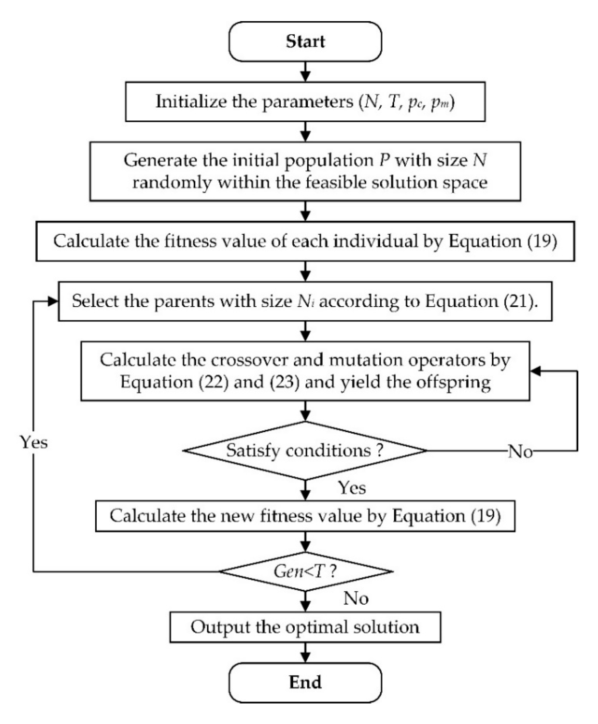
The implementation procedures on solving the joint decision-making model are shown in Figure 4. The detailed instructions of IGA are described as follows.
Step 0: Initialize the parameters of population quantity N , the maximum iteration number T , the probabilities of crossover p c and mutation p m .
Step 1: Generate the initial population P randomly within the feasible solution space obtained by constraints.
Step 2: Calculate the fitness value of each individual according to the objective function Equation (19).
Step 3: Select the parents P 1 (population quantity N i ) from the current population according to Equation (21).
Step 4: Generate the offspring P 2 obtained in Step 3 according to the following steps.
Step 4.1: Calculate the crossover and mutation operators based on Equations (22) and (23) to yield the offspring P 2 .
Step 4.2: Check whether the individual in the offspring P 2 satisfies the constraints. If it satisfies the conditions, proceed to the next step; otherwise, return to Step 4.1.
Step 5: Calculate the fitness value of each individual in the offspring P 2 again based on Equation (19).
Step 6: Check the current iteration number G e n . If G e n   <   T , then return to Step 3; otherwise, output the optimal solution.

5. Numerical Experiments

The numerical results of the joint model and proposed algorithm are reported in this section. In Section 5.1, a basic numerical experiment with one tomato farm and 20 consumer nodes is carried out to verify the efficiency of the joint model. In Section 5.2, the optimal solutions of joint model and traditional model are compared in terms of vehicle number, penalty cost and distribution cost. In Section 5.3, the results of sensitivity analysis on penalty cost and time window are reported. In Section 5.4, the performance of improved genetic algorithm (IGA) is examined from aspects of iteration number and CPU time. All experiments are performed on an Intel Core i3-8100 3.60 GHz processor with 16 GB RAM and MATLAB 2017a.

5.1. Basic Numerical Experiments

There are one tomato farm and 20 consumer nodes in this case. The geographic locations, expected maturity and demand quantities are all known. The unit earliness and tardiness penalty costs are set as: γ 1 = 0.05   CNY / unit , γ 2 = 0.2   CNY / unit , ϑ 1 = 0.1   CNY / unit , ϑ 2 = 0.4   CNY / unit . The unit picking time ( α ) is set to 50   kg / h . The IGA parameters are set as: N = 100 , T = 1000 , p c = 0.9 and p m = 0.05 . There are two vehicle types used in this study, and q 1 = 100   kg , q 2 = 70   kg . The unit fixed usage and unit distribution costs are set as: f 1 = 130   CNY , f 2 = 100   CNY , ω 1 = 2.2   CNY / h and ω 2 = 2   CNY / h . Figure 5 shows the spatial coordinate of each node (citing from Solomon [39]). The tomato farm is denoted as circle 0 , and the consumer nodes are denoted as circle 1 ~ 20 . Table 4 gives the information of consumer orders on geographic locations, tomato demands and expected maturity.
The basic numerical experiment is tested 10 times, and the optimal tomato picking and distribution scheduling is shown in Table 5 and Figure 6. There are four vehicles used in this scheduling to distribute the tomatoes, three vehicles are type 1 and one vehicle is type 2. The v1-1 in Figure 6 represents the vehicle 1 with type 1. In this scheduling, vehicle 1 with type 1 serves consumer 1, consumer 9, consumer 20, consumer 3, consumer 12 in turns, and then returns to the tomato farm. The total cost is 1610.57 CNY, where maturity penalty cost is 295.94 CNY, and distribution cost is 1314.63 CNY.

5.2. Comparison between Joint Model and Traditional Model

To further analyze the economic contribution of the joint model, the optimal result is compared with the traditional distribution scheduling. According to models reported by Cordeau et al. [40] and Koc et al. [41], the traditional model is formulated as a cost-based model, which does not consider maturity time window and penalty cost. In the proposed model, the time windows are generated from the tomato maturity model to constrain picking and distribution decision. However, in the traditional distribution mode, the distribution cost is the primary factor for retailers to make decisions. The time window [ e i r , l i r ] in the joint model is slacked to formulate the traditional model (i.e., e i r = 0 , l i r = M ). That is to say, the maturity penalty cost is not considered in the traditional distribution mode. In the traditional model, the optimization objective is to minimize the delivery cost for order fulfillment.
The optimal objective values of the traditional model are shown in Table 6 and Figure 7. The vehicle number is 3 and the distribution cost is 1138.92 CNY. Compared with the results of joint model, the vehicle number and distribution cost are reduced. Without the time window constraints, the retailer arranges the vehicles only considering loading capacities and geographical locations. To calculate the penalty cost of traditional model, tomato arrival times at consumers in the traditional scheduling are introduced into Equation (4). The maturity penalty cost of traditional model is 829.06 CNY, which is 2.8 times that of the joint model. In summary, the joint model could reduce the maturity penalty cost by 64.30% and save the total cost by 357.41 CNY in this case setting. The comparison results demonstrate that the joint model could provide a precise scheduling to satisfy the consumer requirements.

5.3. Sensitivity Analysis on Maturity Penalty and Time Window

In this study, the tomato maturity time windows are calculated by multiple experiments on tomato samples. Considering different fruits have different maturity characteristics, it would bring stricter or more inclusive time window restrictions, as well as affect picking and distribution decisions. For example, the maturity speed of peaches is faster than that of tomatoes, so that the maturity time window intervals are smaller. In this context, the retailer needs to fulfill the peach orders in a shorter time. Therefore, in this subsection, the sensitivity analyses are carried out in terms of maturity penalty factors and maturity time windows.
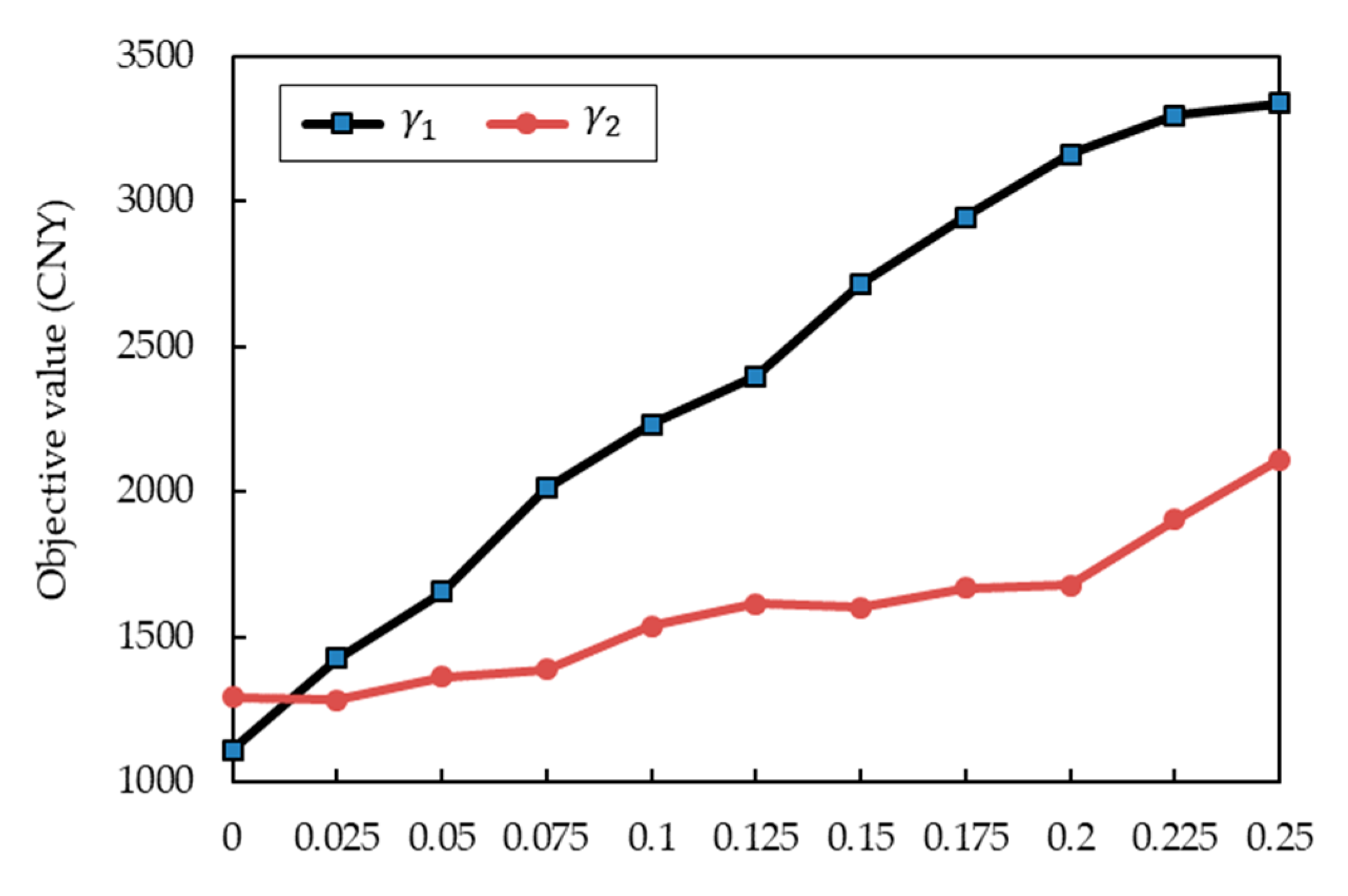
For maturity penalty, the unit earliness penalty cost ( γ 1 ) and tardiness penalty cost ( γ 2 ) are varied from 0 to 0.25 in interval of 0.025, respectively. As shown in Figure 8, with the increase of γ 1 and γ 2 , the objective value increases gradually. It can be seen that the increase rate of the objective value by increasing γ 1 is higher than that by increasing γ 2 . The variation trend demonstrates that the maturity speed of tomatoes is relatively slow than other fruits, and most of the maturity penalty costs in this scheduling are earliness penalty. It could provide more distribution time for retailers to satisfy the expected maturity. In addition, to satisfy the increasing requirements of consumers, the retailer would weigh the penalty cost and distribution cost to reduce the total cost.
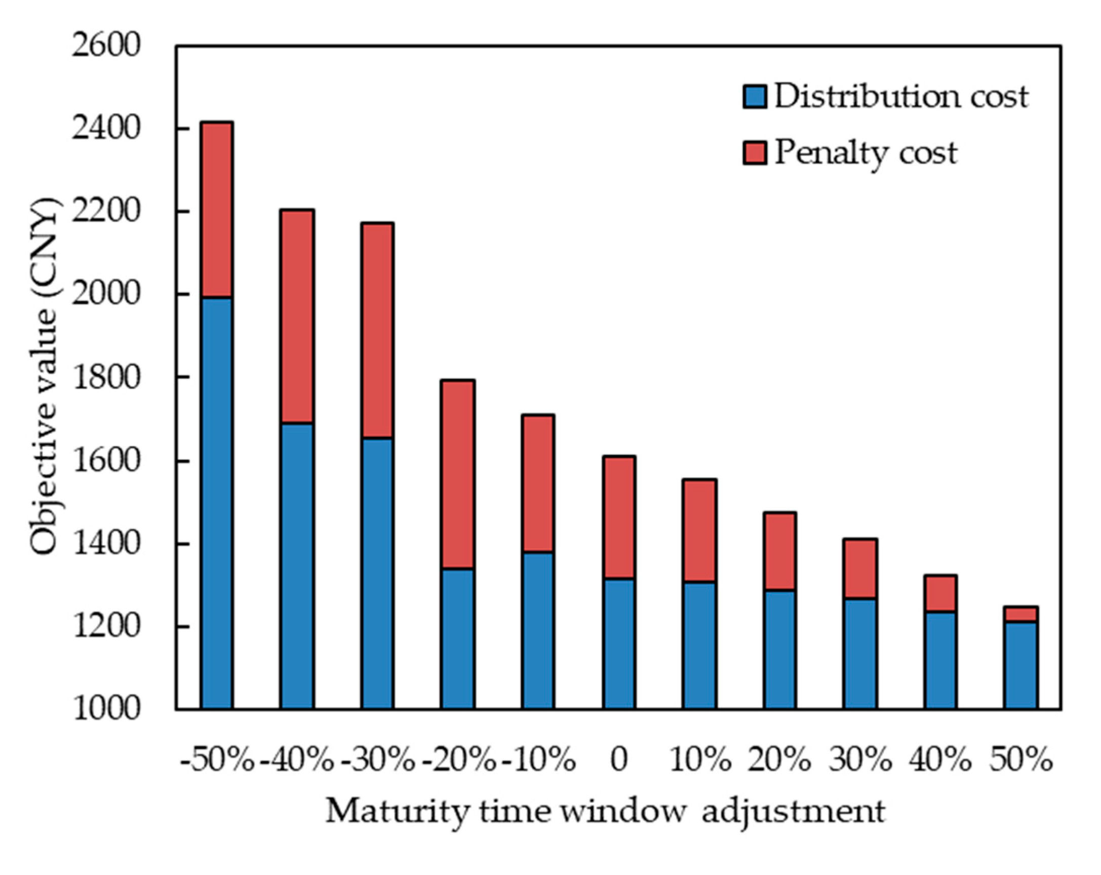
For the maturity time window, the interval of each time window is adjusted by ± 10 % , ± 20 % , ± 30 % , ± 40 % and ± 50 % . If the initial time window is 0–50, the adjusted time windows are 0–45 by adjusting 10 % , and 0–55 by adjusting + 10 % . The results are reported in Figure 9. With the time window shrinking, the objective values increase gradually. When the time window intervals are large enough, the distribution costs have slight gaps, such as adjusting the time windows by 30%−50%. In these cases, the routing scheduling is mainly determined by distribution cost constraints. However, when time window intervals are small, the retailer needs to assign more vehicles or adjust the most economical routing to satisfy the maturity requirements. The distribution cost would increase greatly with strict time window constraints, which demonstrates that the retailer needs to assign more vehicles to distribute fruits to reduce the penalty possibility. In addition, the distribution cost in case of time window −10% is higher than case of time window −20%. Although the stricter time constraint leads to a higher penalty cost, it may bring more total costs by increasing the vehicle number. Therefore, the retailer could weigh distribution cost and penalty cost to determine the least total cost scheduling.
In general, retailers could adjust the distribution strategy according to the fruit maturity characteristic and consumer demand preference. Three managerial insights could be drawn from numerical analyses above:
  • For some fruits with higher maturity rates, distribution in advance could avoid a sharp drop in consumer satisfaction.
  • For some fruits with slower maturity speed rates, consumers are more inclined to receive fruits with closer maturity, rather than immature fruits; thus, a delayed distribution could reduce the penalty cost.
  • Retailers could shorten the distribution time by increasing the vehicle number to satisfy strict maturity requirements of consumers.

5.4. Medium-to-Large Scale Numerical Experiments

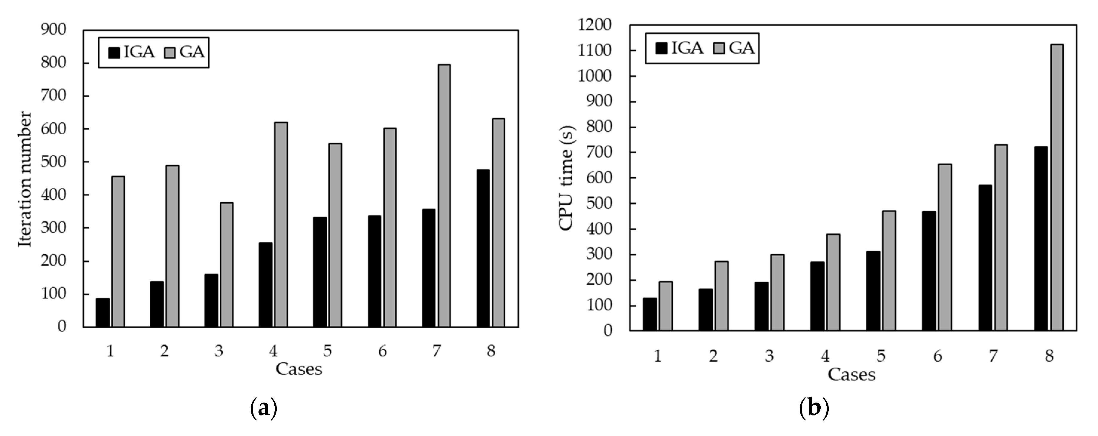
Considering the large number of online orders and scattered demand locations, it is crucial to calculate a feasible solution in a reasonable time. The proposed IGA aims to provide the optimal solution quickly for retailers in practice. To further verify the efficiency of the proposed algorithm, eight medium-to-large scale cases are tested. The consumer number increases from 30 to 100. The computational performance results of IGA and genetic algorithm (GA) are reported in terms of CPU time and iteration number.
As shown in Figure 10a, the iteration number of IGA ranges from 80 to 500. With the scale of numerical experiment increasing, the iteration number would increase accordingly. While the iteration number of GA ranges from 350 to 800, which is significantly greater than IGA. In Figure 10b, CPU times of IGA are all less than that of IGA. Especially for solving the large-scale numerical case with 100 consumer nodes, CPU time of IGA is 714 s, while that of GA is 1123 s. In this case, IGA saves about 7 min of solution time. Generally, the proposed IGA converges the optimal solution with fewer iterations and shorter time. Compared with GA, the IGA proposed in this study saves an average of 32.37% CPU time and reduces the iteration number by 54.27% on average. The joint decision-making model and proposed IGA have superior in solving the medium-to-large scale cases, which is feasible for practical application.

6. Conclusions

This study proposes a joint decision-making approach for tomato picking and distribution considering postharvest maturity. To satisfy diversified maturity requirements, a postharvest maturity model is formulated by monitoring variations of firmness and SSC. The maturity time windows are calculated and introduced into picking and distribution processes. An optimization model is proposed by joining picking decision and distribution scheduling to ensure that orders could be fulfilled within the optimal maturity time window. This model represents a feasible method to address the high-quality deterioration and diverse requirements of fresh agri-product online retailing, especially for climacteric fruits. An economical distribution scheduling is proposed to satisfy requirements by overlapping maturing time and distribution time. Moreover, numerical experiments demonstrate that the proposed IGA saves iteration number and CPU time by 54.27% and 32.37% on average compared to GA. In general, this proposed method could take full advantage of postharvest maturity data to provide more decision-making possibilities for retailers, which has promising applications for tomato online retailing.
This study contains new directions for further research in fruit supply chain considering maturity. On one hand, fruit has different postharvest maturity speeds in different environments, such as temperature, ethylene, humidity. Investigating the relationship between these factors and postharvest maturity speed could optimize inventory decisions, which is conducive to extending shelf life and improving marketability. On the other hand, for several fruits with short shelf life (such as peach, kiwi and mango), it is economical to make bundle pricing decisions in advance based on maturity stages and speeds. The sales strategies based on maturity provide more available time for retailers, which could reduce quality deterioration and unsalable risk.

Author Contributions

Conceptualization, Z.Z. and Y.J.; investigation, Y.J. and B.B.; methodology, Z.Z., Y.J. and B.B.; supervision, Y.J.; validation, Y.J.; writing—original draft preparation, Y.J. and B.B.; writing—review and editing, Z.Z. and Y.J. All authors have read and agreed to the published version of the manuscript.

Funding

This research has been supported by the National Natural Science Foundation of China (71803084), the Humanity and Social Science Youth Foundation of Ministry of Education of China (17YJC630048) and Fundamental Research Funds for the Central Universities (NAU: SKCX2020009).

Conflicts of Interest

The authors declare no conflict of interest.

Appendix A

Table A1. Notation explanations.
Sets
N Set of nodes including one tomato farm and multiple consumers.
N Set of consumer nodes, N = N / { 0 } .
P Set of vehicle types.
K Set of vehicles.
R Set of tomato maturity stages.
Parameters
γ 1 Unit increase rate of earliness penalty cost.
γ 2 Unit increase rate of tardiness penalty cost.
ϑ 1 Constant earliness penalty cost.
ϑ 2 Constant tardiness penalty cost.
f p Fixed usage cost of vehicle type p .
ω p Unit distribution cost of vehicle type p .
n p Number of type p vehicles.
q p Loading capacity of vehicle type p .
α Unit picking time of tomatoes.
d i Tomato demand quantity of consumer i .
τ i j Distribution time between consumer i and j .
[ e i r ,   l i r ] Time window of consumer i with expected tomato maturity r .
Variables
x i j p k Binary decision variable. If x i j p k = 1 , vehicle k with type p serves from consumer i to consumer j .
y i p k Binary decision variable. If y i p k = 1 , consumer i is served by vehicle k with type p .
t i p k Arrival time of vehicle k with type p at consumer i .
t s i p k Start picking time of vehicle k with type p for consumer i order.
t f i p k Finish picking time of vehicle k with type p for consumer i order.

References

  1. Testa, R.; Migliore, G.; Schifani, G.; Tinebra, I.; Farina, V. Chemical-physical, sensory analyses and consumers’ quality perception of local vs. imported loquat fruits: A sustainable development perspective. Agronomy 2020, 10, 870. [Google Scholar] [CrossRef]
  2. Porat, R.; Lichter, A.; Terry, L.A.; Harker, R.; Buzby, J. Postharvest losses of fruit and vegetables during retail and in consumers’ homes: Quantifications, causes, and means of prevention. Postharvest Biol. Technol. 2018, 139, 135–149. [Google Scholar] [CrossRef] [Green Version]
  3. Vinyes, E.; Asin, L.; Alegre, S.; Muñoz, P.; Boschmonart, J.; Gasol, C.M. Life cycle assessment of apple and peach production, distribution and consumption in Mediterranean fruit sector. J. Clean. Prod. 2017, 149, 313–320. [Google Scholar] [CrossRef]
  4. Macheka, L.; Spelt, E.; van der Vorst, J.G.A.J.; Luning, P.A. Exploration of logistics and quality control activities in view of context characteristics and postharvest losses in fresh produce chains: A case study for tomatoes. Food Control 2017, 77, 221–234. [Google Scholar] [CrossRef]
  5. Ge, H.; Gray, R.; Nolan, J. Agricultural supply chain optimization and complexity: A comparison of analytic vs simulated solutions and policies. Int. J. Prod. Econ. 2015, 159, 208–220. [Google Scholar] [CrossRef]
  6. Ahumada, O.; Rene Villalobos, J.; Nicholas Mason, A. Tactical planning of the production and distribution of fresh agricultural products under uncertainty. Agric. Syst. 2012, 112, 17–26. [Google Scholar] [CrossRef]
  7. Widodo, K.H.; Nagasawa, H.; Morizawa, K.; Ota, M. A periodical flowering—Harvesting model for delivering agricultural fresh products. Eur. J. Oper. Res. 2006, 170, 24–43. [Google Scholar] [CrossRef]
  8. Van de Poel, B.; Bulens, I.; Hertog, M.L.A.T.; Van Gastel, L.; De Proft, M.P.; Nicolai, B.M.; Geeraerd, A.H. Model-based classification of tomato fruit development and ripening related to physiological maturity. Postharvest Biol. Technol. 2012, 67, 59–67. [Google Scholar] [CrossRef]
  9. Desrosiers, J.; Dumas, Y.; Solomon, M.M.; Soumis, F. Chapter 2 Time Constrained Routing and Scheduling. In Handbooks in Operations Research and Management Science; Elsevier: Amsterdam, The Netherlands, 1995; Volume 8, pp. 35–139. [Google Scholar]
  10. Cattaruzza, D.; Absi, N.; Feillet, D.; Vigo, D. An iterated local search for the multi-commodity multi-trip vehicle routing problem with time windows. Comput. Oper. Res. 2014, 51, 257–267. [Google Scholar] [CrossRef]
  11. Wang, Z.; Li, Y.; Hu, X.P. A heuristic approach and a Tabu search for the heterogeneous multi-type fleet vehicle routing problem with time windows and an incompatible loading constraint. Comput. Ind. Eng. 2015, 89, 162–176. [Google Scholar] [CrossRef]
  12. Hu, B.X.; Sun, D.W.; Pu, H.B.; Wei, Q.Y. Recent advances in detecting and regulating ethylene concentrations for shelf-life extension and maturity control of fruit: A review. Trends Food Sci. Technol. 2019, 91, 66–82. [Google Scholar] [CrossRef]
  13. Farina, V.; Gentile, C.; Sortino, G.; Gianguzzi, G.; Palazzolo, E.; Mazzaglia, A. Tree-ripe mango fruit: Physicochemical characterization, antioxidant properties and sensory profile of six Mediterranean-grown cultivars. Agronomy 2020, 10, 884. [Google Scholar] [CrossRef]
  14. Hussain, A.; Pu, H.B.; Sun, D.W. Innovative nondestructive imaging techniques for ripening and maturity of fruits—A review of recent applications. Trends Food Sci. Technol. 2018, 72, 144–152. [Google Scholar] [CrossRef]
  15. Schouten, R.E.; Huijben, T.P.M.; Tijskens, L.M.M.; van Kooten, O. Modelling quality attributes of truss tomatoes: Linking colour and firmness maturity. Postharvest Biol. Technol. 2007, 45, 298–306. [Google Scholar] [CrossRef]
  16. Olarewaju, O.O.; Bertling, I.; Magwaza, L.S. Non-destructive evaluation of avocado fruit maturity using near infrared spectroscopy and PLS regression models. Sci. Hortic. 2016, 199, 229–236. [Google Scholar] [CrossRef]
  17. Sun, Y.D.; Singh, Z.; Tokala, V.Y.; Heather, B. Harvest maturity stage and cold storage period influence lemon fruit quality. Sci. Hortic. 2019, 249, 322–328. [Google Scholar] [CrossRef]
  18. Kasampalis, D.S.; Tsouvaltzis, P.; Siomos, A.S. Chlorophyll fluorescence, non-photochemical quenching and light harvesting complex as alternatives to color measurement, in classifying tomato fruit according to their maturity stage at harvest and in monitoring postharvest ripening during storage. Postharvest Biol. Technol. 2020, 161, 111036. [Google Scholar] [CrossRef]
  19. Zhai, Z.Y.; Martínez, J.F.; Beltran, V.; Martínez, N.L. Decision support systems for agriculture 4.0: Survey and challenges. Comput. Electron. Agric. 2020, 170, 105256. [Google Scholar] [CrossRef]
  20. Ferrer, J.; Mac Cawley, A.; Maturana, S.; Toloza, S.; Vera, J. An optimization approach for scheduling wine grape harvest operations. Int. J. Prod. Econ. 2008, 112, 985–999. [Google Scholar] [CrossRef]
  21. Arnaout, J.M.; Maatouk, M. Optimization of quality and operational costs through improved scheduling of harvest operations. Int. Trans. Oper. Res. 2010, 17, 595–605. [Google Scholar] [CrossRef]
  22. An, K.; Ouyang, Y. Robust grain supply chain design considering post-harvest loss and harvest timing equilibrium. Transp. Res. Part E Logist. Transp. Rev. 2016, 88, 110–128. [Google Scholar] [CrossRef] [Green Version]
  23. Munoz, F.; Lee, S. Sugarcane harvest scheduling using a distributed control approach. Procedia Manuf. 2019, 39, 1149–1157. [Google Scholar] [CrossRef]
  24. Hu, H.T.; Zhang, Y.; Zhen, L. A two-stage decomposition method on fresh product distribution problem. Int. J. Prod. Res. 2017, 55, 4729–4752. [Google Scholar] [CrossRef]
  25. Bortolini, M.; Faccio, M.; Ferrari, E.; Gamberi, M.; Pilati, F. Fresh food sustainable distribution: Cost, delivery time and carbon footprint three-objective optimization. J. Food Eng. 2016, 174, 56–67. [Google Scholar] [CrossRef]
  26. Wang, X.P.; Wang, M.; Ruan, J.H.; Zhan, H.X. The multi-objective optimization for perishable food distribution route considering temporal-spatial distance. Procedia Comput. Sci. 2016, 96, 1211–1220. [Google Scholar] [CrossRef] [Green Version]
  27. Alenazi, M.M.; Shafiq, M.; Alsadon, A.A.; Alhelal, I.M.; Alhamdan, A.M.; Solieman, T.H.I.; Ibrahim, A.A.; Shady, M.R.; Saad, M.A.O. Non-destructive assessment of flesh firmness and dietary antioxidants of greenhouse-grown tomato (Solanum lycopersicum L.) at different fruit maturity stages. Saudi J. Biol. Sci. 2020. [Google Scholar] [CrossRef]
  28. USDA. United States Standards for Grades of Fresh Tomatoes. Available online: http://agris.fao.org/agris-search/search.do?recordID=US201300356169 (accessed on 11 June 2013).
  29. Beckles, D.M. Factors affecting the postharvest soluble solids and sugar content of tomato (Solanum lycopersicum L.) fruit. Postharvest Biol. Technol. 2012, 63, 129–140. [Google Scholar] [CrossRef]
  30. Huang, Y.P.; Lu, R.F.; Chen, K.J. Assessment of tomato soluble solids content and pH by spatially-resolved and conventional Vis/NIR spectroscopy. J. Food Eng. 2018, 236, 19–28. [Google Scholar] [CrossRef]
  31. Cherono, K.; Workneh, T.S.; Melesse, S.F. Application of logistic statistical modelling in the evaluation of suitable conditions for the supply of fresh tomatoes in selected South African supply chains. Int. Food Res. J. 2019, 26, 979–989. [Google Scholar]
  32. De Ketelaere, B.; Lammertyn, J.; Molenberghs, G.; Desmet, M.; Nicolai, B.; De Baerdemaeker, J. Tomato cultivar grouping based on firmness change, shelf life and variance during postharvest storage. Postharvest Biol. Technol. 2004, 34, 187–201. [Google Scholar] [CrossRef]
  33. An, X.; Li, Z.G.; Zude-Sasse, M.; Tchuenbou-Magaia, F.; Yang, Y.G. Characterization of textural failure mechanics of strawberry fruit. J. Food Eng. 2020, 282, 110016. [Google Scholar] [CrossRef]
  34. Wang, H.T.; Zhang, R.Y.; Peng, Z.; Jiang, Y.L.; Ma, B.X. Measurement of SSC in processing tomatoes (Lycopersicon esculentum Mill.) by applying Vis-NIR hyperspectral transmittance imaging and multi-parameter compensation models. J. Food Process Eng. 2019, 42, e13100. [Google Scholar] [CrossRef]
  35. Sheng, R.; Cheng, W.; Li, H.H.; Ali, S.; Agyekum, A.A.; Chen, Q.S. Model development for soluble solids and lycopene contents of cherry tomato at different temperatures using near-infrared spectroscopy. Postharvest Biol. Technol. 2019, 156, 110952. [Google Scholar] [CrossRef]
  36. Koulamas, C. Common due date assignment with generalized earliness/tardiness penalties. Comput. Ind. Eng. 2017, 109, 79–83. [Google Scholar] [CrossRef]
  37. Wang, Z.Z.; Sobey, A. A comparative review between Genetic Algorithm use in composite optimisation and the state-of-the-art in evolutionary computation. Compos. Struct. 2020, 233, 111739. [Google Scholar] [CrossRef]
  38. Thinkaran, N.; Jayaprakash, J.; Elanchezhian, C. Optimization of total cost in inventory routing problem with homogenous type of vehicles using metaheuristic algorithm—A review. Mater. Today Proc. 2019, 16, 1043–1047. [Google Scholar] [CrossRef]
  39. Solomon, M.M. Algorithms for the vehicle-routing and scheduling problems with time window constraints. Oper. Res. 1987, 35, 254–265. [Google Scholar] [CrossRef] [Green Version]
  40. Cordeau, J.F.; Laporte, G.; Savelsbergh, M.W.P.; Vigo, D. Chapter 6 Vehicle routing. In Handbooks in Operations Research and Management Science; Elsevier: Amsterdam, The Netherlands, 2007; Volume 14, pp. 367–428. [Google Scholar]
  41. Koc, C.; Bektas, T.; Jabali, O.; Laporte, G. Thirty years of heterogeneous vehicle routing. Eur. J. Oper. Res. 2016, 249, 1–21. [Google Scholar] [CrossRef] [Green Version]
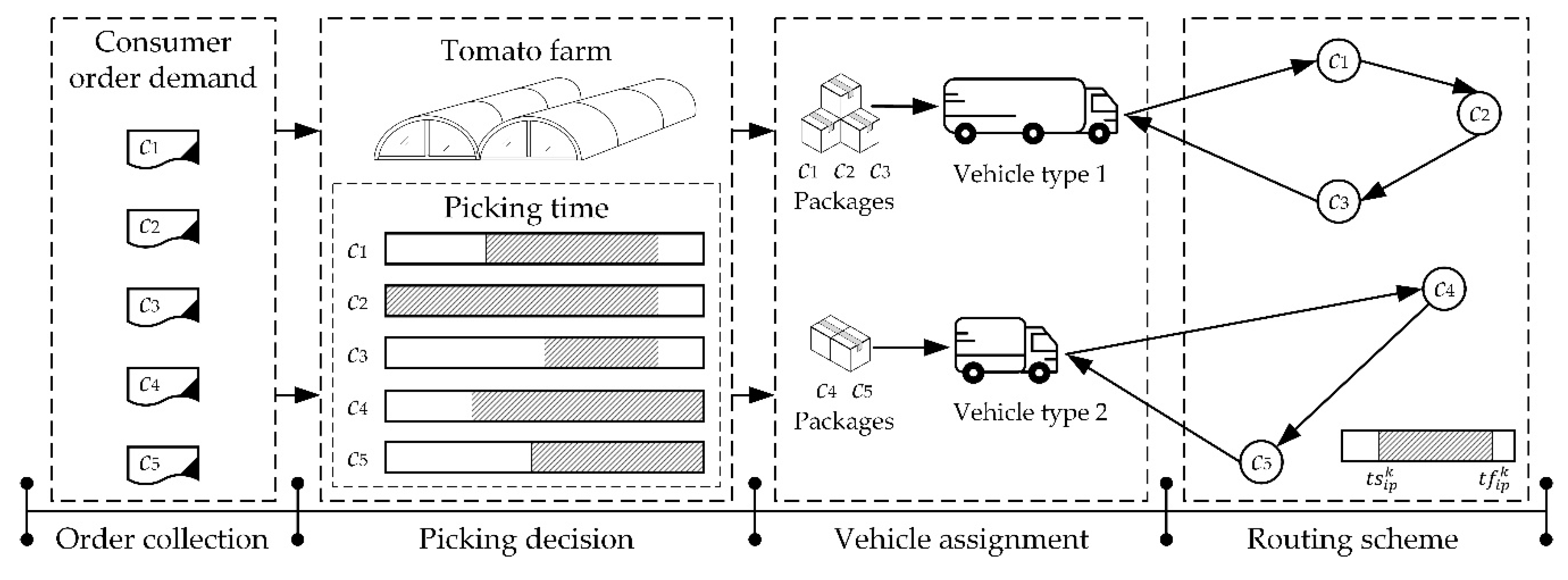
Figure 1. Diagram for picking and distribution for tomato online retailing based on postharvest maturity.
Agronomy 10 01330 g001
Figure 2. Tomato samples at five maturity stages. (a) Breaker stage; (b) Turning stage; (c) Pink stage; (d) Light red stage; (e) Red stage.
Agronomy 10 01330 g002
Figure 3. Data distribution of tomato maturity indices at different maturity stage. (a) Firmness index. (b) SSC index.
Agronomy 10 01330 g003
Figure 4. Flow chart of the improved genetic algorithm (IGA).
Agronomy 10 01330 g004
Figure 5. Schematic diagram of spatial coordinates of tomato farm and consumers.
Agronomy 10 01330 g005
Figure 6. Schematic diagrams of the optimal vehicle routing.
Agronomy 10 01330 g006
Figure 7. Cost values of the optimal scheduling from joint model and traditional model.
Agronomy 10 01330 g007
Figure 8. Relationship between the unit penalty cost and the objective value.
Agronomy 10 01330 g008
Figure 9. Relationship between the time window and the objective value.
Agronomy 10 01330 g009
Figure 10. Comparison of computational performance between GA and IGA. (a) Comparison of iteration number between GA and IGA; (b) comparison of CPU time between GA and IGA.
Agronomy 10 01330 g010
Table 1. Statistical analysis of firmness and soluble solid content (SSC) maturity indices a.
Maturity IndexMaturity Stage
BreakerTurningPinkLight redRed
Firmness40.09 ± 1.69 A35.22 ± 1.93 B32.27 ± 2.04 C27.74 ± 1.30 D25.48 ± 1.81 E
SSC4.71 ± 0.20 E5.14 ± 0.15 D5.34 ± 0.15 C5.70 ± 0.19 B6.09 ± 0.22 A
a Values in this table is defined as average value ± standard deviation. A–E Superscripts A–E represent the significant difference between different maturity stages by the analysis of variance. If superscripts are different in one row, the maturity index has significant differences between these two maturity stages.
Table 2. Curve regression analysis for tomato maturity and time.
Maturity ModelEquation R 2 S i g .
FirmnessQuadratic0.9270.001
SSCExponential0.8560.011
Table 3. Time windows for tomato different maturity base on firmness.
Maturity StageFirmness Value Range Time Window ( h )
Breaker37.9–42.30–44
Turning33.1–37.944–65
Pink28.5–33.165–80
Light red25.9–28.580–88
Red22.1–25.988–98
Table 4. Consumer order information.
NumberCoordinate
( k m )
Demand
( k g )
Expected
Maturity a
NumberCoordinate
( k m )
Demand
( k g )
Expected
Maturity a
0 [ 35 ,   35 ] 0011 [ 20 ,   65 ] 122
1 [ 41 ,   49 ] 10412 [ 50 ,   35 ] 195
2 [ 35 ,   17 ] 7413 [ 30 ,   25 ] 233
3 [ 55 ,   45 ] 13414 [ 15 ,   10 ] 203
4 [ 55 ,   20 ] 19515 [ 30 ,   5 ] 274
5 [ 15 ,   30 ] 26116 [ 10 ,   20 ] 194
6 [ 25 ,   30 ] 21217 [ 5 ,   30 ] 145
7 [ 20 ,   50 ] 17218 [ 20 ,   40 ] 125
8 [ 10 ,   43 ] 9319 [ 15 ,   60 ] 172
9 [ 55 ,   60 ] 16420 [ 45 ,   65 ] 313
10 [ 30 ,   60 ] 162
a The corresponding relationship between maturity stage and numbers is: Break = 1, Turning = 2, Pink = 3, Light red = 4, Red = 5.
Table 5. Optimal tomato picking and distribution scheduling.
Vehicle TypeVehicle NumberThe Optimal Vehicle Routing
Type 1Vehicle 10→1→9→20→3→12→0
Vehicle 20→7→10→11→19→8→17→18→0
Vehicle 30→6→13→2→15→4→0
Type 2Vehicle 10→5→16→14→0
Objective value o b j 1 o b j 2 Total CostNumber of Vehicles
295.94 CNY1314.63 CNY1610.57 CNY4
Table 6. Comparison results of the joint model and traditional model.
ModelObjective Value
Number of Vehicles o b j 1 o b j 2 Total Cost
Joint model4295.94 CNY1314.63 CNY1610.57 CNY
Traditional model3829.06 CNY1138.92 CNY1967.98 CNY