The R Package PROSPER: An Environment for Modeling Weed Population Dynamics and the Evolution of Herbicide Resistance

Abstract

Weed management is a challenge for farmers worldwide, and the problem is exacerbated by the spread of weed herbicide resistance. Simulation models that combine population dynamics and genetics are valuable tools for predicting the impact of competing management options on weed density, allele frequency, and phenotypic resistance levels. The new R package PROSPER provides functions for the forward simulation of weed population dynamics on a field scale, the selection of individuals according to their sensitivity to herbicides, and the recombination of alleles during reproduction. Objects are provided to enter and save model parameters in a clear structure, and to save output data for further processing in R. The basic functions are extensible with R code. PROSPER combines individual-based population dynamics with monogenic or polygenic diploid inheritance and flexible selection pressure. Stochasticity can be included at all model steps. Two examples of the population dynamics of two annual weed species with herbicide resistance are presented. All parameters and the models are available in PROSPER. In addition to simulation, PROSPER is intended for sharing and publishing population dynamic parameters and models, which is easily done thanks to R.

1. Introduction

The management of annual arable weeds is a long-term challenge for farmers. Weed infestation is and will remain a permanent issue because weed species have evolved special strategies to survive and evade the frequent disturbances in arable fields: due to high weed reproduction rates combined with seed longevity, weeds establish large soil seed banks [1,2], which are buffered from depletion by seed dormancy [3]. The seed bank may be regarded as a memory; it transfers such population “experience” as seed abundances and genetic constitution, for example, in the context of herbicide sensitivity, to the following years [3,4].

Because of the long-term nature of changes in abundance and population characteristics, and because of the threat to productivity posed by weeds, simulation models are used worldwide to predict the dynamics of weed populations [5]. The influence of alternative treatments on abundances as well as phenotypic and genotypic characteristics can be examined by simulation. Computer simulations also support planning field trials and complement them for the efficient allocation of research resources. However, programming simulation models is time consuming, and weed researchers are mostly not trained in programming. Therefore, a couple of basic functions and simple but easily expandable computer simulation models can assist researchers in overcoming this shortcoming.

Here, our objective is to present the R package PROSPER (population dynamics Rostock-PERTH), which combines functions and objects to build forward, that is, predictive, simulation models [6]. This package supports the development of very diverse models. The structures of population dynamic models differ considerably depending on their objectives [5,7]. PROSPER aims to simplify the development of weed models that enable the study of the interplay between population dynamics and genetics under the influence of weed management. A particular focus is on the development of herbicide resistance.

With regard to the Colbach [7] model overview, PROSPER models are mechanistic models with empirically derived demographic parameters to examine long-term dynamics. Typical users are scientists who intend to close gaps in knowledge and organize research. Additionally, PROSPER aims to be used by agriculture and ecology students. Regarding Holst’s [5] division of model approaches, PROSPER models simulate the population dynamics of one annual weed species, including a seed bank with discrete time steps from one life history stage to the next. Life stages are linked by germination, survival, and reproduction. The occurrence of several cohorts, which is typical for many arable weed species, can be simulated simultaneously. Density dependence and stochasticity can be implemented at each stage transition. The models combine intra-annual changes, which are especially important for management questions, and inter-annual population changes, which are ecologically relevant. This link between short-term and long-term dynamics enables the important study of the long-term effects of crop management [8]. An individual field forms the spatial basis of a model. Spatial population dynamics within and between fields are not yet included. The influence of the abiotic environment and of weed and crop management is implicitly modeled by using appropriate empirical life-stage transition functions. Competition with the crop can be simulated explicitly. As to the genetic component of the evolutionary dynamics, PROSPER models follow Renton’s [9] idea of an individual-based approach for diploid organisms. Polygenic expression (up to four alleles) of phenotypic characteristics with variable degrees of gene dominance and epistatic effects (interaction of genes) is enabled.

Adopting predefined models facilitates simulation model programming. Therefore, at present, PROSPER includes codes and parameters of three published models: PERTH (polygenic evolution of resistance to herbicides), a model developed for herbicide resistance in Lolium rigidum Gaudin [10], which has been proven in subsequent studies to be useful [11,12,13,14] and which was an inspiration for the development of the PROSPER package; one model for Echinochloa crus-galli (L.) P. Beauv. in maize fields [15]; and one for Galium aparine L. in winter wheat [16]. This collection can be extended to distribute new models rapidly and with maximum transparency. PROSPER thus also provides a platform to publish weed population dynamic parameters and models.

After having pointed out the relevance of population-dynamic weed models and having classified PROSPER models into the world of these models (Section 1), we first present the concept of a model within PROSPER (Section 2): we show how the population is described and in what manner the diverse development steps constitute a reproduction cycle. Then, we continue by presenting the workflow for the implementation of the model in the R package PROSPER (Section 3), which is followed by two practical examples (Section 4). Finally, we discuss our approach (Section 5) and provide conclusions as well as an outlook for PROSPER (Section 6).

2. The Concept of a PROSPER Simulation Model

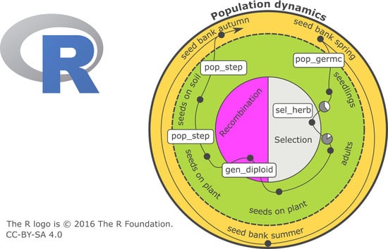
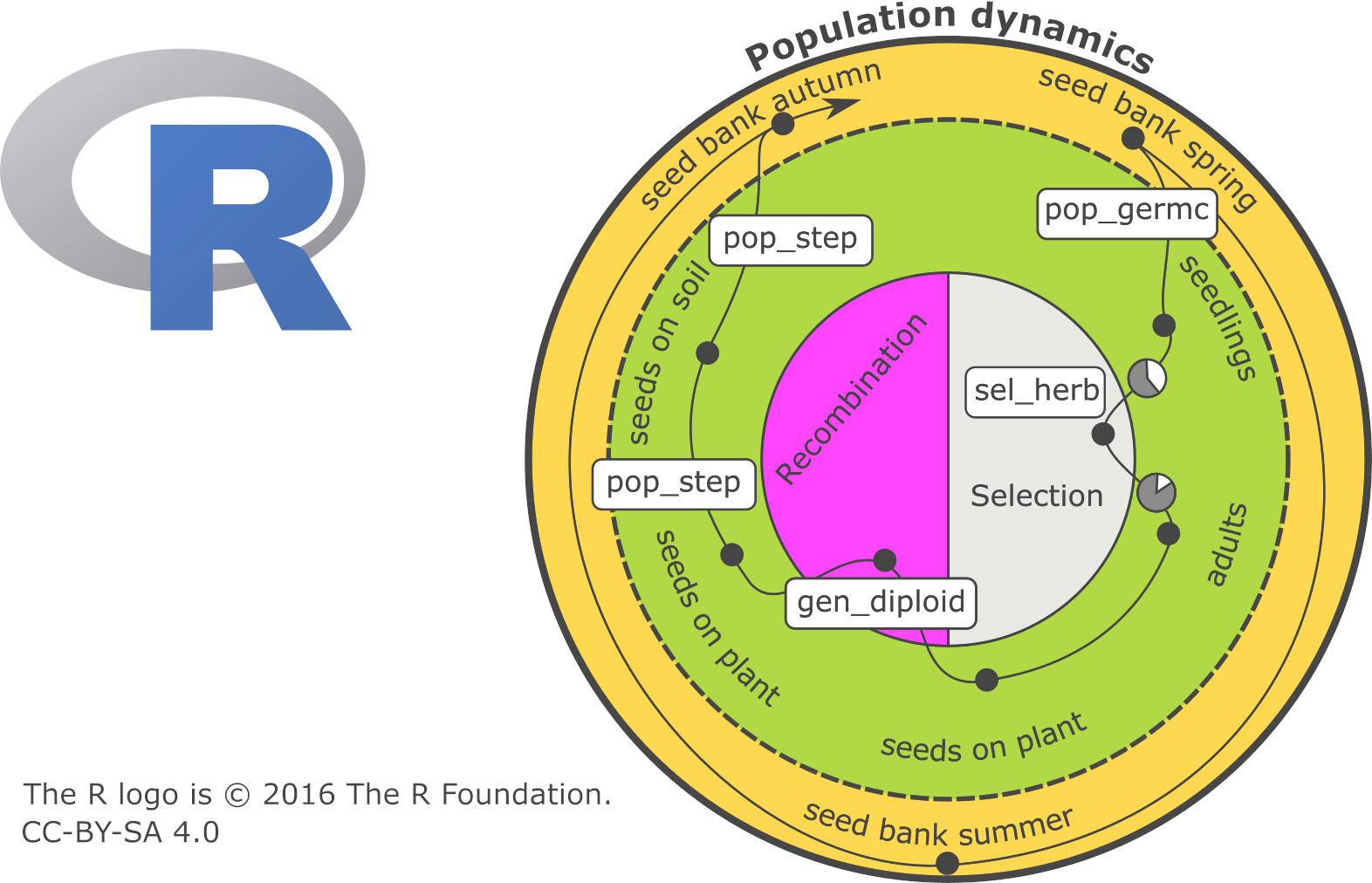
The first focus of a PROSPER model is on weed population dynamics. A schematic representation of a PROSPER model is shown in Figure 1. The large circle symbolizes the sum of the weed individuals that form the population and the eternal cycle of the generation sequence of a population. An individual plant successively passes through development stages, from a seed in soil to death (black points in Figure 1) and new seed production. The arrow displays the timely sequence of these development stages. Different cohorts are represented by splitting branches. For weed species that build a seed bank, at least two cohorts evolve: one greening above the soil and one resting as a seed in the soil (e.g., Figure 1). Many weed populations have only one reproductive cycle during the course of one year, while others have more.

The development of a population takes place in discrete development steps, in which every single plant is individually handled/treated. Three qualitatively different steps are distinguished:

• Surviving through the development stage and entering the following stage.
• Splitting the population by building new cohorts. Usually, germination is the first cohort-building process.
• Reproduction, including the production of new seeds.

On their path through the generation cycle, individual plants can experience special events, which are coded by two additional functions:

4.

Selection (right side of the inner circle in Figure 1) concerns the probability of an individual surviving and entering a new development stage. Since PROSPER provides an individual-based framework, every simulated seed or plant has a specific genetic profile. Whether an individual survives depends on its susceptibility to the selection pressure. Individual susceptibility is caused by genetic disposition, which is the composition, action, and interaction of relevant alleles in genetic material. Different processes can exert selection pressure. In conventional agriculture, herbicides are important selecting agents. Their effects are usually described using nonlinear dose–response models, for example, the log-logistic function [17].

5.

Reproduction/recombination (left side of the inner circle in Figure 1) is currently limited to four gene loci in a diploid population, and alleles are freely combinable. As in the selection process, recombination takes place at the level of individuals.

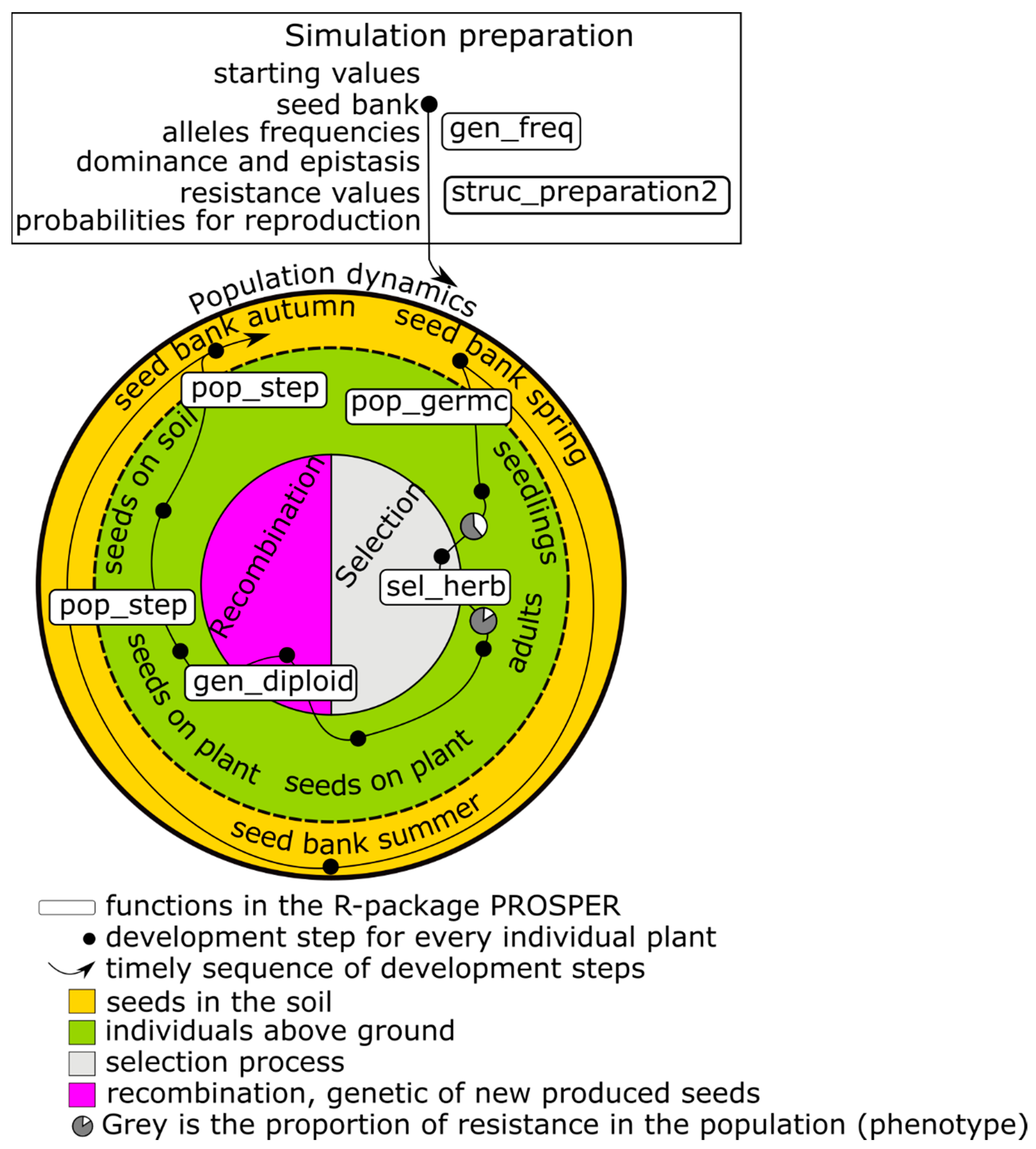
The initialization of state variables and the parameterization of transition functions are necessary before population development can be simulated (upper box in Figure 1). The simulation begins in most cases at a point at which all individuals are in the stage “seeds in the soil”—as usual with annual weeds. Nevertheless, it is possible to start the simulation at any parameterized stage. The weed specific parameters are linewise stored in a table (i.e.,

Table 1. Parameters for a population dynamic simulation of Echinochloa crus-galli [15]. These include in this case proportions with variation (here, only for surv_seedling1) or without (e.g., germ1) and hyperbolic functions (e.g., seed_prod_first).

Weed	Crop	Step	Name	Estimate	Std.Error	Model	Range_Low	Range_Up	Source
ECHCG	corn	germ1	intercept	0.08	0.00				[21]
ECHCG	corn	germ2	intercept	0.04	0.00
ECHCG	corn	surv_seedling1	start	0.68	0.02				[22]
ECHCG	corn	seed_prod_first	a1	200	0.00	a1*x/(exp(C1*t1) + a*x/B1)			[23]
ECHCG	corn	seed_prod_first	t1	1.00	0.00
ECHCG	corn	seed_prod_first	C1	0.50	0.00
ECHCG	corn	seed_prod_first	B1	2 × 105	0.00
ECHCG	corn	seed_prod_second	a2	100	0.00	a2*x/(exp(C2*t2) + a2*x/B2)			[23]
ECHCG	corn	seed_prod_second	t2	2	0.00
ECHCG	corn	seed_prod_second	C2	0.50	0.00
ECHCG	corn	seed_prod_second	B2	3 × 104	0.00
ECHCG	corn	seed_surv_winter	intercept	0.80	0.00				[24]
ECHCG	corn	seed_surv_summer	intercept	0.10	0.00				[24]
ECHCG	corn	seed_pred	intercept	0.65	0.00	0.92			[24,25]

). From the minimum of one vital rate, the table can be extended for parameters of any other desired crops, farming methods, and life circle processes. In many cases, these parameters differ within a crop rotation with the crop [18]. Therefore, they need to be assigned for each crop in the simulated crop rotation. All other parameters, including tillage or fertilizer, are directly included in the individual steps. Hence, if tillage affects the germination of a specific weed, tillage must be included in the model for the germination step (i.e., Table 1 the model at step germ1 should include tillage). Whether a crop is tilled or whether a selection agent is present in a specific simulation cycle must be defined by the simulation model itself. A possible way to include the tillage is shown in Supplementary Materials (Example S1), where we present a reconstructed part of a matrix model [19], which simulates weed population dynamics in an agricultural system with four crops and three different tillage measures [20].

3. The Workflow to Get a Model

At the very beginning of every modeling attempt, it is necessary to define what is modeled and for what reason, after which the necessary modeling steps for that specific case can be defined. Depending on the user demands, PROSPER offers the possibility of using already existing models in the package, modifying these models, or setting up new models. The usual workflow to produce a population dynamic simulation model is as follows. First, the parameters defining each step must be provided (the parameterization of the model). In the second and third steps, the model must be initialized, and the actual simulation is conducted. Finally, the output is analyzed. A minimal example of the workflow is provided in the Supplementary Materials (Example S2).

3.1. Parameterization: Preparing the Data

One specific step of a simulation model such as seed production [26] or seed predation [27] can be described by simple rate variables or more complex statistical models with or without variation—the transition function. The state variables of the step are determined via pot or field trials and can include management, climate, and plant-specific parameters as well as any other relevant variable. During parameterization, it is of great importance to use the same units as the model for the current step. Using PROSPER, all these population dynamic parameters must be collected in the data frame param.weed with a predefined structure. This data.frame must be loaded into the model function. Table 1 presents an example of E. crus-galli, which is used in Section 4. In each line, one parameter is described by providing the names of the weed and the crop, the weed development step (“step”) to which it belongs, its name (“name”), its role in a transition function (“model”), its estimated value (“estimated”), and, optionally, its standard error (“std.error”). These values and standard errors are the result of analyzed experiments. If they are already published, the reference is cited in the column “source”. Limits of the parameter values can be given in the columns “range_low” and “range_up”. When programming, all model parameters concerning the simulation setting can be entered within the call of PROSPER functions. These parameters include genetic information, herbicide effects, competition with a crop, duration and areal scope, and number of model runs, if stochasticity is included.

3.2. Initialization of the Model

First, during the model initialization within PROSPER, the data frame dfgenotype, a data-saving structure which includes the phenotypic resistance values for each possible genotype, is generated. Genetic recombination probabilities for each possible genotype are calculated and tabulated. During the simulations, these values are not calculated again but rather looked up in the table. This is the only step that is done only once, even in case of several simulation runs, due to stochasticity. Next, the initial number of individuals for the model must be entered or generated from the weed parameter table param.weed. These individuals are assigned to the possible genotypes (gen_freq()). Because this step can include stochasticity, it is repeated in each simulation run. Individuals are characterized by their alleles, and the allocation of alleles to the individuals equals the frequency of alleles in the population. The calculation of the phenotypical susceptibility against selecting events depending on the genotype is time consuming. Therefore, the phenotypical responses are calculated and listed in a table for all possible combinations of alleles with their respective dominance and epistasis properties. Thus, the susceptibilities are considered and not recalculated during the simulation process. The function struc_preparation2() generates necessary data-saving objects, which save: (i) the initial values and the simulation results for weed numbers; (ii) probabilities of sexual reproduction resulting in a specific genotype; and (iii) phenotypic resistance values for a specific genetic profile.

3.3. Simulation Cycle and Stochasticity

While several functions execute the population development, pop_step() is the one used most often. It needs values, numbers, or proportions, which can be generated by the function quanti(). This PROSPER function enables the results of experiments to be directly introduced into the simulation model using more or less complex algorithms, for example, linear models including variance, during the simulation. These algorithms can incorporate the complete farming system, including elements such as soil, weather, and crop rotation. For weeds, the algorithms used are density-dependent in many cases; quanti() accesses the data from the table param.weed (Table 1) with the weed population dynamic parameters.

While quanti() in combination with pop_step() provides one important source of stochasticity, there are two other sources within the simulation cycle. One is reproduction. During reproduction, adults and alleles are selected randomly, resulting in a population with a specific distribution of genotypes, each with specific resistance values. The selection process, the last source of stochasticity, compares the herbicide rate reaching each individual plant with the resistance value derived from the individual genetic profile. The herbicide rate reaching the plant is a random value of a normal distribution representing the uncertainty of in-field herbicide application caused, for example, by the position of plant leaves within canopy or drift. In addition, every plant can completely escape the herbicide treatment by chance. These processes follow the PERTH model [10].

The result for every step in one reproduction cycle is stored in dfgenotype as a separate column. At the end of one reproduction cycle, the function struc_saveSimData() saves the resulting dfgenotype to the object sim_result and prepares dfgenotype for the next cycle. Therefore, the last result column of the last step during one cycle becomes the starting column of the next cycle.

3.4. Exploring the Simulation Results

All results are collected in the data frame object “sim_result”. There, the number of individuals in all development steps, all years, and all genotypes is accessible for all simulation cycles and repetitions of the simulation. The scientific questions raised in weed science are diverse. Therefore, PROSPER provides only simple summarizing functions (plot() and summary()) and leaves a more detailed analysis to the user.

4. Two Example Simulations

An important feature of PROSPER is to collect and distribute population dynamic models. Every modeler is invited to modify these or add new models to let this collection “prosper”. In the current version, three fully parameterized and previously published models are incorporated. The model on L. rigidum is a reconstructed PERTH model which was built to assess the sustainability of weed management with reduced herbicide doses (for details, see [10]). The model on E. crus-galli [15] investigates how seeds of late-emerging weeds affect the evolution of herbicide resistance. For G. aparine, a simulation was run to determine whether sowing seeds of sensitive weeds is a promising approach to lower the resistance status of a field population [16]. All models are simplified; that is, no crop rotations or changing weather conditions are included. A minimal example is provided in the supplements.

4.1. Effect of Late-Emerging Echinochloa crus-galli Cohorts on Herbicide Resistance

E. crus-galli is one of the most frequent weeds found in maize fields in Germany [28,29] and a relevant threat to maize yields [30]. Numerous herbicide-resistant populations are reported worldwide [31]. E. crus-galli is able to germinate over a long period after maize planting, though with decreasing reproductive success [24]. In the model (Figure 2a), all germinating individuals are represented by two cohorts: an early major cohort with high seed production and a small late cohort emerging with lower reproduction. 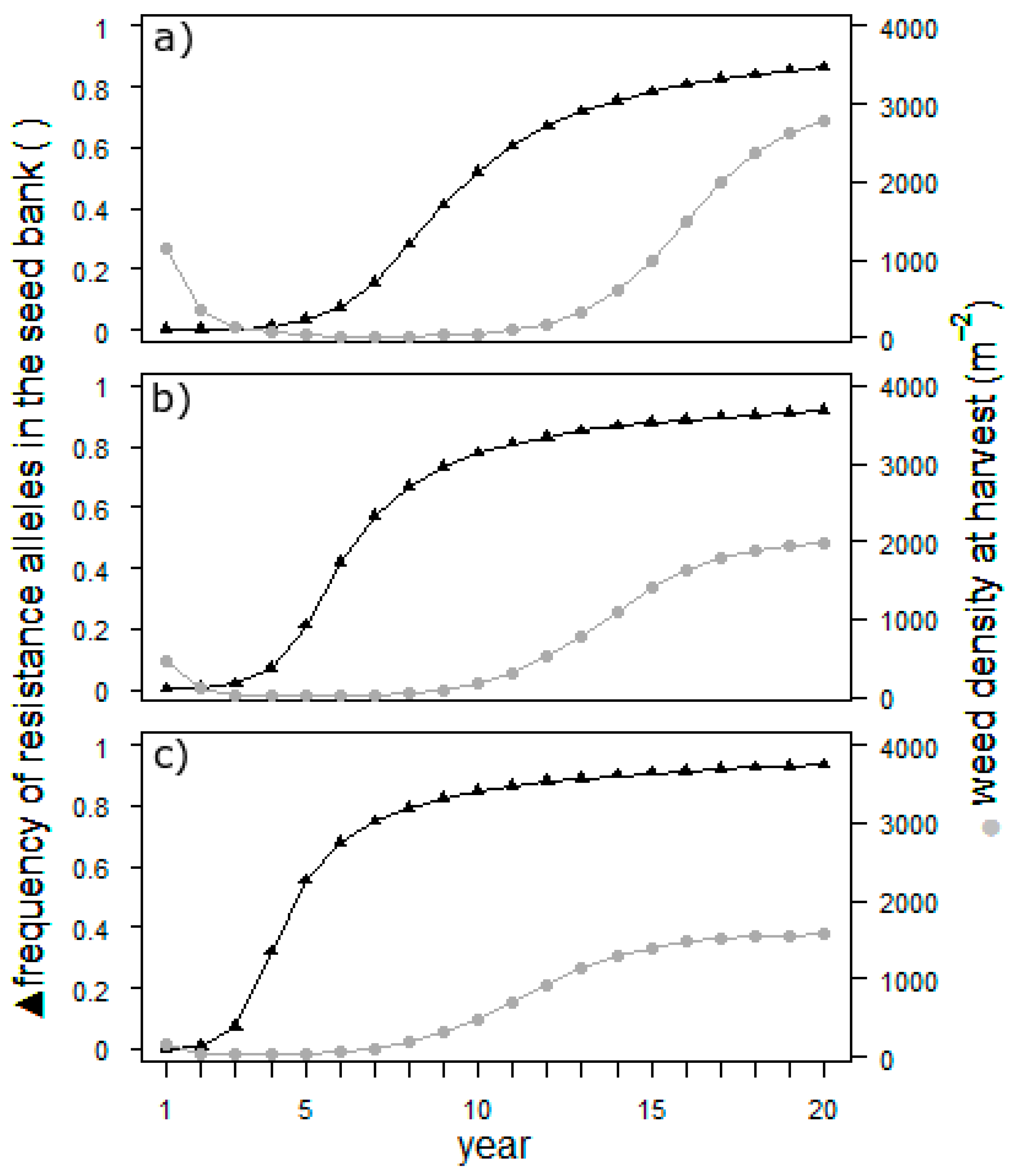Only the first cohort is controlled by a herbicide, which is a typical situation in Germany [32]. The second cohort escapes the herbicide treatment unaffected. However, the second cohort can be suppressed in terms of survival as well as fecundity, for example, by an undersown crop. Three scenarios with different degrees of suppression, 0%, 30%, and 100%, were simulated [15].

To simplify the model setup in this example, a target site resistance was assumed with an initial frequency of the dominant resistance allele of 0.001. Epistatic effects were excluded. Simulations for each of the scenarios ran over 20 years and were repeated 15 times.

The results in Figure 3 illustrate that, regardless of the suppression, the weed population will be almost 100% resistant after 20 years. Resistance will, however, develop nearly twice as rapidly in the scenario with complete suppression of the second cohort than in the zero-suppression scenario. Hence, later-germinating individuals of E. crus-galli have a high potential to buffer the development of herbicide resistance in the field. The development of the weed density mirrors the efficiency of weed control. As long as the resistance is low and herbicide treatment is effective, the density is low. As soon as the resistance is high, the population begins to grow exponentially to an unacceptable density. The density reached in the end of the simulation depends on the suppression of the second cohort. The population size is known to be an important factor for the development of herbicide resistance. If the sensitivity of late-emerging cohorts is incorporated into the resistance management of a field, it is important to track the resistance level: as soon as it rises, the density will follow. For the management of herbicide resistance, this effect potentially could be used. However, the main measures are others [18], with the most important being not to change the herbicide mode of action.

4.2. Restoring a Susceptible Population Status of Galium aparine

Whether the sowing of susceptible weed seeds can restore an “acceptable” resistance level of a population in the early stages of resistance development is an interesting and practice-oriented research question. Until today, herbicide resistance in G. aparine has only been reported in China and the Middle East [31]. The patchy occurrence of this weed species and its large seeds result in highly variable population dynamic parameters. Modeling must take this variability into account. We used a simple population dynamic model structure [16]. A seedbank in spring provides seeds out of which one cohort germinates. The weeds are selected by herbicides; produce seeds, which are affected by seed predation; and return to the seedbank in the autumn (Figure 2b). Data from a long-term field experiment were used for parameterization [25].

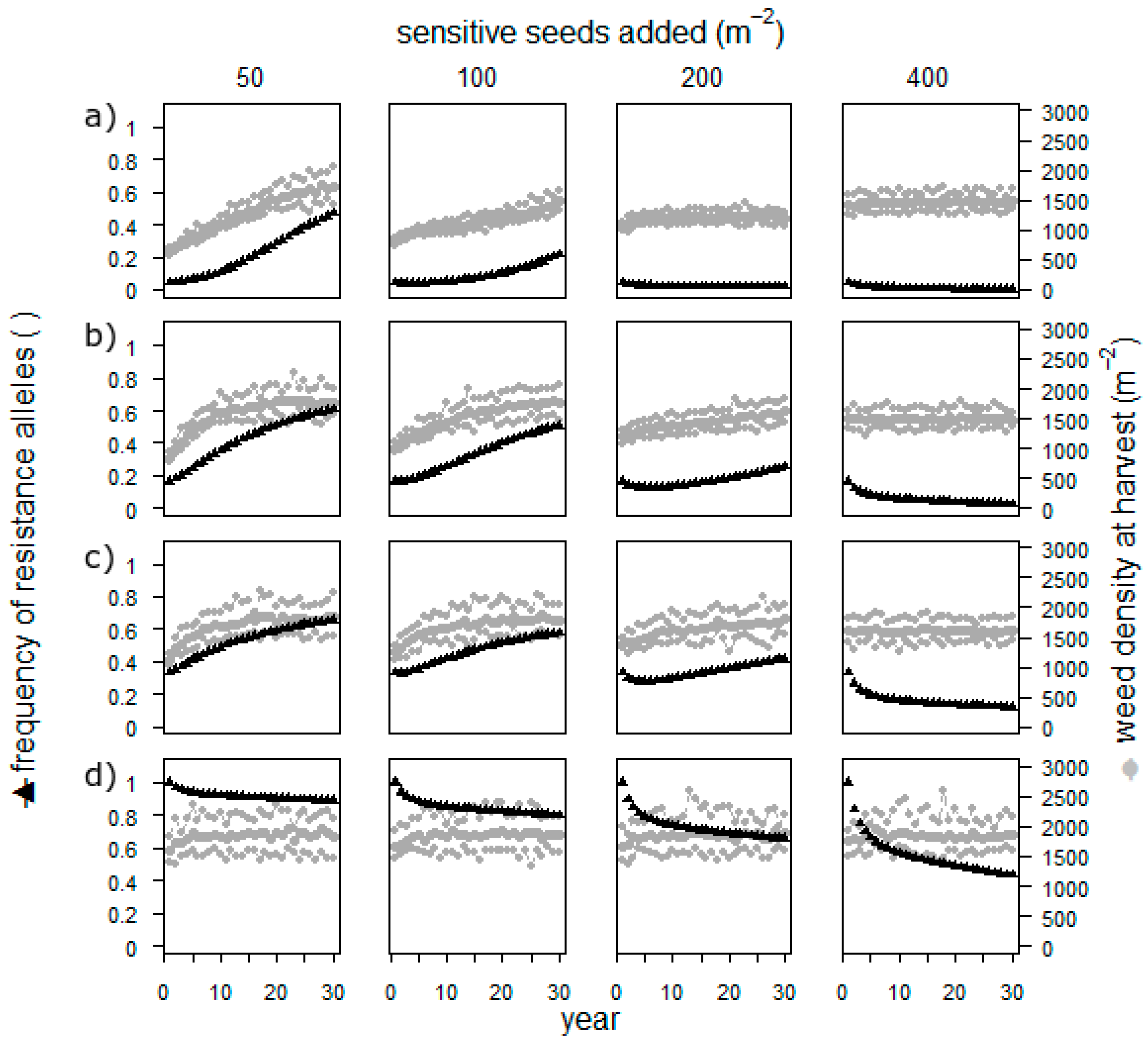
We simulated the development of metabolic herbicide resistance using three resistance genes without epistasis and co-dominance for all genes. Metabolic resistance is thus described with the approach of polygenic inheritance [10,33] without considering changing gene expression. The initial seedbank was 2285 seeds/m². We used four levels of yearly added seeds (50, 100, 200, and 400 seeds/m²) and four levels of herbicide resistance in the field, stretching from nearly 0% (frequencies were 0.03, 0.08, and 0.02 for the three resistance alleles) to 100% resistant alleles. Each of the resulting 16 scenarios was simulated over 30 years and repeated 20 times.

Sowing sensitive seeds resulted in populations with a low or nearly exhausted resistance when the frequency of resistant alleles was low in the beginning (Figure 4). When the starting frequency of resistant alleles was high, even the highest applied number of added seeds did not cure the field. The weed density, however, remained high throughout the simulation in all scenarios.

The approach to add weed seeds to a field is thus not highly realistic, and the assumptions on reproduction and fecundity are rough estimates. However, it is possible, and simulation is the perfect way to investigate the potential effect. Adding seeds has an effect only as long as the herbicide resistance is not yet high. It thus seems impossible to cure the field once the resistance is established. Furthermore, the weed density is always very high, which makes a direct usage of this measure in herbicide resistance management impossible. Thus, before establishing field experiments, researchers should address this by conducting further simulations such as removing the selection process for several years.

5. Discussion

PROSPER has basic tools to formulate population dynamic models for weeds and is intended to serve as a distribution platform for published models. Such an attempt has been made in the past [34,35]. The key difference between these attempts and the approach presented here is the use of the freely available language R. Many agricultural scientists are not commonly trained in programming in general, but they are trained to use R for analysis and plotting [36]. With the R package PROSPER, the workflow is completed in one environment: the estimation of parameters, the simulation, and the analysis and presentation of the results are all done with R. PROSPER saves all results in one object, which makes the handling easy even for non-programmers. This all-in-one approach gives PROSPER, written in R, an advantage compared to similar platforms such as “WeedML” written in C++ [34] or “simuPOP” written in Python [35,37]. We agree with the other authors that a common platform significantly enhances the development of population dynamic models, and we believe that R can be the correct path to achieve this. Therefore, PROSPER can be received by the authors and is published at CRAN [6].

Within the large world of R, several packages deal with population dynamics [38] and some are prepared to be used for weeds [39]. We could have expanded one of the existing packages; however, we decided to develop a new R package completely dedicated to weeds and population dynamics because of the very complex nature of weed population dynamics. The complex mixture of natural and managed/controlled processes can cause specific reactions and makes a particular adoption of the models inevitable.

Aside from the complexity of population dynamics, the basic structure of a simulation model with PROSPER is always similar, which makes them easy to read. This structure is based on the PERTH model [10]. This simply structured but powerful model and its presentation have been successfully used in teaching and introducing population dynamics, as well as modeling, to students. Therefore, PROSPER has the potential to be used in teaching as well. In addition, the possibility to adopt models contained in the package facilitate the start of population dynamic modeling.

The examples show two cases of population dynamic modeling with PROSPER. Both include a very simple monoculture cropping system. In that way, the results evolve more rapidly and are much more stable. The examples prove the effectiveness of combining all relevant variables—management, climate, and soil—of one specific development step in one statistical model. In addition, both are examples which provide practical hints for science: late-emerging cohorts have the potential to slow the development of herbicide resistance. A sufficient number of added seeds can even “cure” herbicide resistance at very low levels. In both cases, an experiment could follow the simulation and could be focused on the relevant scales at the low level of herbicide resistance in the field.

6. Conclusions and Outlook

PROSPER enables easy establishment of population dynamic models. However, some functions are missing, such as a quick check of the settings, a helper function to create a model skeleton, or a sensitivity analysis. These functions are in progress and, once added, will hopefully further increase the usability of PROSPER. Furthermore, the following extensions are planned: (1) spatial differentiation, which is known to affect selective processes [12]; (2) additional processes and ways of selection; and (3) an alternative description of genetics and mating. With these extensions more complex questions can be engaged such as mixing the selection effects of diversified management or a better adaption to a specific weed can be reached. The most important objective is: (4) new models and parameterizations. With a growing collection of models, the usability of PROSPER will grow rapidly, and adapting the models to new research questions will become increasingly easy.